Incorporating nonlinear relationships in microarray missing value imputation

Abstract

Microarray gene expression data often contain missing values. Accurate estimation of the missing values is important for down-stream data analyses that require complete data. Nonlinear relationships between gene expression levels have not been well-utilized in missing value imputation. We propose an imputation scheme based on nonlinear dependencies between genes. By simulations based on real microarray data, we show that incorporating non-linear relationships could improve the accuracy of missing value imputation, both in terms of normalized root mean squared error and in terms of the preservation of the list of significant genes in statistical testing. In addition, we studied the impact of artificial dependencies introduced by data normalization on the simulation results. Our results suggest that methods relying on global correlation structures may yield overly optimistic simulation results when the data has been subjected to row (gene) – wise mean removal.

I. Introduction

Microarray and other high-throughput data often contain missing values that hamper the application of many unsupervised and supervised learning techniques. A number of methods were developed for the imputation of the missing values, some of which were reviewed and compared by Brock et al [1]. Most imputation methods stem from the observation that the relationship between gene expression levels can be approximated by linear models. There are two broad classes of imputation methods. The first class utilizes local information, i.e. neighbors of the gene of interest. A representative of this class is the widely used K-nearest neighbor (KNN) method, which fills the missing value by the weighted average of the expression of K neighboring genes in the same array [2]. The LSimpute method applies linear regression between the gene with missing value and neighboring genes [3]. Robust regression using the principal components of the neighbors was also proposed [4]. Local least squares (LLS) imputation uses multiple regression of the gene with missing value against the neighboring genes [5]. The method often achieves optimal performance with a very large number of neighbors, some times over 50% of the genes in the array [1, 5]. This suggests the method partly takes advantage of the global correlation structures between arrays. A multi-stage clustering method which incorporates missing value imputation was also proposed [6]. The second class of imputation methods utilizes the global correlation structure. The SVD method uses the dependency of the experiments on the first several singular vectors of the data matrix to impute the missing values [2]. A more complex and better performing variant, BPCA, uses probabilistic PCA and Bayesian estimation [7]. To go beyond the linear relationship between experiments, the Support Vector Regression imputation maps the samples to higher dimensional space with kernel functions [8].

In addition to using a single imputation scheme, the idea of ensemble learning has been applied, in which imputed values from multiple methods were combined [9–11]. Another way of improving imputation accuracy is to recruit external information. Examples include the use of other microarray datasets from the same organism [12], functional annotation of genes [13], knowledge of synchronization loss in time-series data [14], and epigenetic information [15].

Dependencies between genes can be complex and far from linear [16, 17]. General dependency has been shown to be effective for the inference of gene regulatory networks [17–19]. These results suggest that non-linear relationships between genes are biologically relevant, and may provide extra information in missing value imputation. A parametric non-linear regression method has been proposed to utilize such information, which however still preselects neighboring genes based on Euclidean distance [20]. Here we present a missing value imputation scheme that follows the nearest neighbor principal. The definition of “neighbors” is broadened to incorporate nonlinear dependency. The method is based on both Pearson’s correlation coefficient and a new metric for detecting nonlinear relationships, named similarity based on conditional ordered list (SCOL). For neighbors selected by SCOL, the points corresponding to the expression levels may not be geometrically close to each other. Consequently, the imputation is done using the principle of estimating non-linear response curves by kernel smoother between the gene of interest and its neighbors.

II. METHODS

2.1. Similarity based on conditional ordered list (SCOL)

Here we present a similarity score between two vectors x and y, the purpose of which is to measure the spread of the conditional distribution Y|X in a nonparametric manner. First, each vector is standardized using normal score transformation. The m values of the vector are compared to obtain the ranks R₁, R₂, …, R_m, and then each x_i of the vector is replaced by Φ⁻¹(R_i/(m+1)), where Φ(.) is the cumulative normal distribution. Secondly, we sort the data {(x_i, y_i)} by the X values: $\left\{\left(x_i^{\ast },y_i^{\ast }\right)\right\},x_1^{\ast }\le x_2^{\ast }\le \dots \le x_p^{\ast }$. Thirdly, the sum of absolute differences between the adjacent Y values in the ordered list is obtained as the raw distance,

$$D_{\mathit{col}}(\mathbf{x},\mathbf{y})=\sum _{i=2}^m\left|y_i^{\ast }-y_{i-1}^{\ast }\right|.$$

This is equivalent to summing the Manhattan distances between adjacent points in the list ordered by X, up to a constant. Lastly, the raw distance is standardized such that it is between zero and one. The theoretical minimum of the distance is

$$D_{\mathit{col}}^{min}={\mathrm{\Phi }}^{-1}(m/(m+1))-{\mathrm{\Phi }}^{-1}(1/(m+1)),$$

which is obtained when the two vectors have the exact same rank order. When m is odd, the theoretical maximum possible distance is

$$D_{\mathit{col}}^{max}=2\sum _i\left|{\mathrm{\Phi }}^{-1}(i/(m+1))\right|+{\mathrm{\Phi }}^{-1}((m-1)/2(m+1)).$$

When m is even,

$$D_{\mathit{col}}^{max}=2\sum _i\left|{\mathrm{\Phi }}^{-1}(i/(m+1))\right|+2{\mathrm{\Phi }}^{-1}(m/2(m+1))$$

These maximum possible values are obtained when all the adjacent Y values in the ordered list have opposite signs and the two end y values have the smallest absolute values. To standardize the raw score such that it is between zero and one, we obtain the SCOL similarity by

$$S_{\mathit{col}}^{\mathit{std}}(\mathbf{x},\mathbf{y})=1-\frac{D_{\mathit{col}}(\mathbf{x},\mathbf{y})-D_{\mathit{col}}^{min}}{D_{\mathit{col}}^{max}-D_{\mathit{col}}^{min}}.$$

This SCOL similarity is asymmetric, as it focuses on the spread of Y|X (Fig. 1a & 1b). For the purpose of missing value imputation, we use the asymmetric version $S_{\mathit{col}}^{\mathit{std}}(\mathbf{x},\mathbf{y})$ where Y is the gene with missing value to be imputed and X is any other gene. To obtain a symmetric version for measuring nonlinear relationship, we can take

Figure 1.

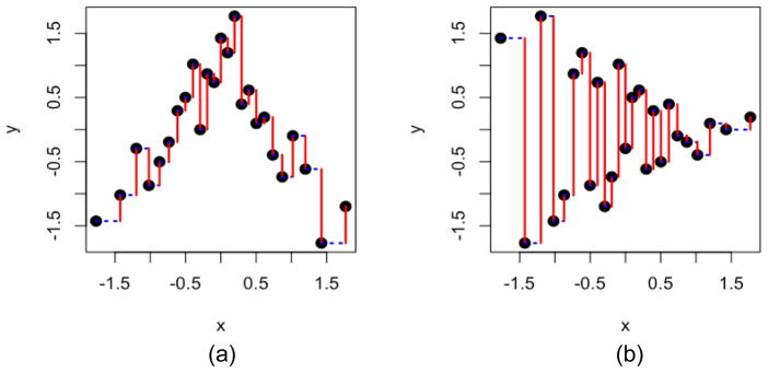
Illustration of the similarity based on conditional ordered list (SCOL). (a) An example where Y and X have a non-linear relationship and the spread of Y|X is small. (b) The same data as in (a) with the role of X and Y reversed, resulting in much lower similarity score because the spread of Y|X is large. Red vertical line segments: distance between adjacent Y values based on the list ordered by the value of X. Blue dotted horizontal line segments: distance between adjacent X values.

$$S_{\mathit{col},\mathit{sym}}^{\mathit{std}}(\mathbf{x},\mathbf{y})=max\left(S_{\mathit{col}}^{\mathit{std}}(\mathbf{x},\mathbf{y}),S_{\mathit{col}}^{\mathit{std}}(\mathbf{y},\mathbf{x})\right).$$

2.2. Selecting informative genes

To impute the missing values of a gene, we utilize both non-linear dependency (measured by SCOL) and linear dependency (measured by the absolute value of Pearson’s correlation coefficient) to select informative genes. The reason for combining CC and SCOL in gene selection is because CC is more responsive when a slight curvature exist, yet the relationship is still monotone, while SCOL is more responsive when the curvature is large and/or the relation is non-monotone.

First, we compute the absolute correlation matrix C and the SCOL matrix B, in which $b_{ij}=S_{\mathit{col}}^{\mathit{std}}\left({\mathbf{g}}_{\mathbf{i}},{\mathbf{g}}_{\mathbf{j}}\right)$. To compute the i^th row in B, we re-order the columns of the expression matrix G_n×m based on the rank order of the i^th gene to generate $G_{n\times m}^{\ast }$. Then absolute differences are taken between adjacent columns of the re-ordered matrix to generate the difference matrix $\mathbf{F}:{\mathbf{f}}_{\mathbf{j}}=\left|{\mathbf{g}}_{\mathbf{j}+\mathbf{1}}^{\ast }-{\mathbf{g}}_{\mathbf{j}}^{\ast }\right|$, j=1, …, m−1. When missing values exist in the i^th gene, the corresponding column of the expression matrix is ignored. There are missing entries in the F matrix caused by missing values in other genes. We then take the row-wise mean values of the F matrix, ignoring missing entries, and multiply by the number of columns of F. After transforming the raw distance values to SCOL scores, the vector is used for the i^th row of the B matrix.

Secondly, for every gene that has missing values, its top k neighbors as defined by absolute CC and top k neighbors as defined by SCOL are found from the corresponding columns of the C and B matrices. Combining these two sets of neighbors gives us the set of informative genes. Overlaps may exist, which means the total number of informative genes may be smaller than 2k. In practice, the optimal k can be selected by masking some observed values and then evaluating the imputation accuracy using different k’s.

2.3. Imputing the missing value

Since nonlinear relations are involved, and each informative gene may show a different response pattern with the gene of interest, we use a procedure based on kernel smoother in conjunction with weighted averaging for the imputation. In steps (i) to (iv) below, we find an imputed value from one informative gene. We use g_x to denote the gene expression profile with a missing value to be imputed, and let g_x1 be missing. We use g_i to denote the expression profile of an informative gene. To simplify the discussion, we assume both expression profiles are non-missing at positions 2, ...., p. Steps (i) to (iii) are simply steps of fitting a kernel smoother. Because our interest is in the fit at the missing value location, only a single point of the kernel smoother is calculated.

1. Find the difference between the non-missing values of the two expression profiles.

   $$d_{ij}=g_{xj}-g_{ij},j=2,\dots ,p$$

   The purpose of using the difference, rather than g_x itself, is to alleviate under-estimation of extreme values when the relation is monotone.

2. Find the weight based on the Gaussian density. Observations with g_ij closer to g_i1 receive higher weights.

   $$w_{ij}=e^{-{\left(g_{ij}-g_{i1}\right)}^2/2{\sigma }_i^2},j=2,\dots ,p$$

   where σ_i is one half of the 1/3 quantile of |g_ij − g_i1|, j = 2, …, p. This ensures that 1/3 of the samples are within 2σ_i and make major contribution to the imputation.

3. Impute the missing value by weighted mean,

   $$\begin{array}{c}{\widehat{d}}_{i1}=\sum _{j=2}^p{d}_{ij}{w}_{ij}/\sum _{j=2}^p{w}_{ij}\\ {\widehat{g}}_{x1}^i={\widehat{d}}_{i1}+g_{i1}\end{array}$$
4. Take the weighted variance of the d vector for a measure of confidence,

   $$s_i^2=\frac{{\displaystyle \sum _{j=2}^p}{w}_{ij}{\left(d_{ij}-{\widehat{d}}_{i1}\right)}^2}{\frac{p-2}{p-1}{\displaystyle \sum _{j=2}^p}{w}_{ij}}$$
5. Merge the imputed values from different informative genes by weighted averaging. The weight has two components: (1) genes that have higher SCOL similarity with the gene of interest receive higher weight, and (2) predictions with smaller weighted variance receive higher weight. We assign the weight by

   $${\delta }_i=1/e^{-6S_{\mathit{col}}^{\mathit{std}}\left(g_i,g_x\right)}{s}_i.$$

The reason the parameter value 6 was chosen for the exponential decay function was that we observed empirically most top neighbors showed similarity scores between 0.5 and 0.9. With the parameter 6, the weight increases roughly 10 fold from an SCOL score of 0.5 to an SCOL score of 0.9. The final imputed value is the weighted average,

$${\widehat{g}}_{x1}=\sum _{i=1}^n{\delta }_i{\widehat{g}}_{x1}^i/\sum _{i=1}^n{\delta }_i$$

where n is the number of informative genes used.

2.4. Simulation study

Datasets

Six datasets were used in the simulation study. They included the B-cell lymphoma profiling data [21], the dataset of yeast transcriptome/translatome comparison [22], the NCI60 cell line gene expression data [23], and the GSE19119 dataset on Atlantic salmon [24]. Two yeast cell cycle time series [25], the alpha factor dataset and the elutriation dataset, were used to probe the effect of data normalization on simulation results in imputation studies. The number of genes/conditions of each dataset is listed in Tables 1 and 2.

Table 1.

Datasets and parameter settings of the simulation study.

Dataset		Alizadeh	Halbeisen	Ross	Tymchuk
Original dimension (genes × experiments)		18432 × 67	9216 × 52	9706 × 60	5299 × 34
Used dimension (genes × experiments)		6042 × 67	7431 × 52	2266 × 60	1617 × 34
Parameter setting	NL (k)	5	5	5	5
	KNN (k)	10	10	15	5
	BPCA*	-	-	-	-
	LLS (k)	1208	2972	2039	1132
	SVD(nPcs)	8	10	6	10

^*The recommended parameter setting was used: #samples - 1.

Table 2.

Datasets and parameter settings for the study of normalization effect.

Dataset		Spellman –alpha factor normalized	Spellman –alpha factor	Spellman – elutriation normalized	Spellman – elutriation	Ross, normalized
Original dimension (genes × experiments)		6178 × 18	6161 × 18	6178 × 14	6161 × 14	9706 × 60
Used dimension (genes × experiments)		4489 × 18	4403 × 18	5766 × 14	5651 × 14	2266 × 60
Parameter setting	NL (k)	10	10	10	10	5
	KNN (k)	10	10	10	10	15
	BPCA*	-	-	-	-	-
	LLS (k)	4040	1761	577	283	906
	SVD(nPcs)	8	4	10	4	8

^*The recommended parameter setting was used: #samples - 1.

Methods compared

Four popular imputation methods were used for comparison. They included the K-nearest neighbor (KNN) method [2], the Bayesian PCA (BPCA) method [7], the local least square (LLS) method [5], and the SVD method [2]. The R implementations of these methods were used, which involved packages “impute” and “pcaMethods” [27]. In the results we refer to our method as “NL”. For NL and KNN, the data matrix (after masking known expression values) was first row (gene)-standardized before the imputation, and the values were transformed back after imputation.

Simulating missing patterns

Different percentages of missing (1%, 5%, 10%, 15% and 20%) were simulated. To simulate data with realistic missing patterns, we used a scheme to learn the missing patterns directly from the real data. For every dataset, we divided the data into two parts – matrix A containing all the genes without any missing value, and matrix B containing genes with missing values. The simulated data was generated from matrix A. Assume matrix A had n rows and m columns, and we targeted to obtain a simulated data matrix with p percent missing values. For every gene g_x in matrix A, we first took a random sample from the Poisson distribution with λ=mp/100 to assign the number of missing entries to the gene. Assume the assigned number of missing entries was l. We then selected all the genes from matrix B that contained l missing entries, and randomly sampled one gene from them, denoted g₁. We then found the positions of the g₁ vector that were missing values, and assigned N/A to the same positions of the g_x vector. By carrying out this procedure for every gene in matrix A, we obtained a simulated matrix A^* that contained p percent missing values.

Parameter setting

A preliminary simulation study was conducted to select the best parameter setting for each method. We tested different values of the tuning parameters at every missing percentage, by repeating the mask-impute procedure three times. The parameter values tested for the NL method were k=5, 10, 15, 20; the values for the KNN method were k=5, 10, 15, 20; the values for LLS were k=5%, 10%, 20%, 30%, ……, 90% of the number of genes of the dataset; the values for SVD were nPcs=2, 4, 6, 8, 10, 15, 20, 30, 40 (up to the number of arrays in the dataset). No parameter selection was done for the BPCA method, because it’s been established that the recommended value for the nPcs parameter, which is the number of samples minus 1, performs the best [7]. Other than the major tuning parameters, we relied on the default of each method for other parameters.

To measure the success of imputation and compare the performance between different parameter settings, we used the normalized root mean squared error (NRMSE),

$$\mathit{nrmse}(\mathbf{y},\widehat{\mathbf{y}})=\frac{\sqrt{\frac{1}{n}{\displaystyle \sum _{i=1}^n}{(y_i-{\widehat{y}}_i)}^2}}{\sqrt{\frac{1}{n-1}{\displaystyle \sum _{i=1}^n}{(y_i-\overline{y})}^2}}$$

It measures the deviation of the imputed values from the hidden true values. For each method, the parameter setting that achieved the lowest average NRMSE in the preliminary simulation study (Table 1 and Table 2) was selected for the larger scale simulation study, in which we repeated the mask-impute procedure 50 times for every dataset at each of the five missing percentage settings.

Comparing the performance

To compare the performance of the methods, we employed two methods. The first was NRMSE. The second method measured the impact of the imputation on the statistical testing results. The general idea was to measure how much the imputation changed the list of significant genes in statistical testing, as compared to the test results generated from the original data without missing values. First, testing was conducted on the complete data, and the list of significant genes taken as the reference. Then after each mask-impute process, the same testing procedure was applied and the list of significant genes was compared with the reference list. The false-positive (FP) and false-negative (FN) counts were analyzed to judge the success of the imputation. It should be noted that the reference list from the original data was not the biological truth. Thus the results measured only relative changes, and the FP and FN counts carried no direct biological interpretation. The idea was that the imputation method should change the list of significant genes as little as possible.

Different statistical tests were selected based on the characteristics of each dataset. All the tests were done on a gene-by-gene basis. After testing, The p-values from all the genes were transformed to false discovery rate (FDR) [28], and genes with FDR less than a threshold (detailed in the Results section) were considered significant. Different FDR cutoffs were selected for different datasets, in order to reach a significant gene list of reasonable size for the assessment of false positives (FP) and false negatives (FN) rates after imputation.

For the B-cell lymphoma profiling (Alizadeh) dataset [21], the main clinical interest was the survival outcome. The accelerated failure time (AFT) model assuming the Weibull distribution was fitted for each gene using the samples with survival information. For the yeast transcriptome/translatome comparison (Halbeisen) dataset [22], we fitted a multiple linear regression model for each gene, with RNA source (transcriptome/translatome) as one predictor, stress treatments as another predictor, and the gene expression value as the response. Because the main interest of the study was the contrast between transcriptome and translatome, we focused on genes significantly associated with the RNA source predictor. For the NCI60 cell line (Ross) dataset [23], a regression model was fitted for each gene, with the tissue origin of the cancer cell lines as the predictor, and the gene expression value as the response. The F-test p-value for the overall fit, which measured the association of the gene expression with the tissue origin, was collected. For the yeast cell cycle time series (Spellman) datasets [25], because the main interest was in genes showing periodic behavior, the Fisher’s exact g test for periodicity [29] was used to identify periodically expressed genes. The only dataset for which no test was performed was the GSE19119 (Tymchuk) dataset [24], as no clear outcome could be used for testing.

III. RESULTS AND DISCUSSIONS

We illustrate the calculation of SCOL in Figure 1. The data points are normal score transformed and ordered by the X values, and the absolute distance between adjacent Y values in the list are summed up (Fig. 1, red bars). After further transformation as described in the Methods section, the SCOL similarity measure is obtained. When the spread of Y|X is small (Fig. 1a), the distances are small and the similarity is high. When the spread of Y|X is large (Fig. 1b), the distances are big and the similarity is low. Clearly SCOL similarity score is asymmetric as demonstrated by the two panels in Figure 1 (same data; role of X and Y reversed). Because in missing value imputation, we only focus on the conditional variance of the gene with a missing value given the value of the informative gene, the asymmetric version of SCOL serves the purpose well. In the case of Figure 1(a), an observed value in X will be helpful to predict the value of Y. Yet in the case of Figure 1(b), an observed value in X will not be as helpful in predicting the value of Y.

Simulation results

By masking observed values at different percentages, we compared the performance of the five methods by finding the NRMSE, and by examining the impact of the imputation on statistical testing results. The results are summarized in Figure 2. With the Alizadeh, Ross and Tymchuk datasets, NL showed an advantage over the other methods in terms of NRMSE, while with the Halbeisen dataset, LLS and BPCA performed better (Fig. 2).

Figure 2.

Simulation results for four datasets based on 50 simulations. The datasets (labeled on the left side) are in rows and the type of results (labeled on top) are in columns. Error bars represent standard errors. No testing was performed for the Tymchuk data, because no clear outcome can be used for testing.

We further explored the impact of the imputation on the selection of significant genes. The list of significant genes after imputation was compared to the reference list generated from the original data. The “false positives” and “false negatives” in the subsequent discussion are only relative to the reference list, not the unknown biological truth. We selected different FDR cutoffs between 0.01 and 0.2 for different datasets in order to achieve a reasonable size of the reference list to facilitate FP and FN analysis (Supporting Table 1). For the Alizadeh dataset, the AFT model was used and the FDR cutoff of 0.2 (corresponding p-value cutoff 0.0025) was chosen, which yielded 65 (1.1%) significant genes. For the Halbeisen dataset, multiple regression was used and the FDR cutoff of 0.01 (corresponding p-value cutoff 0.0016) was chosen, which yielded 1184 (15.9%) significant genes. For the Ross dataset, ANOVA was used and the FDR cutoff of 0.01 (corresponding p-value cutoff 0.0022) was chosen, which yielded 510 (22.5%) significant genes.

The simulation results showed that NL’s lead in NRMSE translated to a lead in FP+FN counts, in both the Alizadeh dataset and the Ross dataset (Fig. 2, column 2). In addition, KNN showed stronger performance in FP+FN counts, as compared to it’s own performance in NRMSE. Interestingly, for the Halbeisen dataset, BPCA and LLS’s lead in NRMSE didn’t translate to a clear lead in FP+FN counts. NL’s performance in FP+FN was extremely close to LLS and BPCA up to 15% missing, while it showed lower average FP+FN counts at 20% missing. Pronounced differences were found between the methods in terms of FP/FN ratio (Fig. 2, column 3). NL was almost always the most conservative in this aspect, producing FP/FN ratios that were low. Using both the Halbeisen dataset and the Ross dataset, NL was the only method producing FP/FN ratios close to 1 (dashed line in the plots, zero in log scale). With high-throughput data, the key concern is controlling the FDR. Hence an imputation method that doesn’t introduce too many false-positives is preferable. In this aspect, NL clearly outperformed the other methods.

The impact of row-wise mean removal on the evaluation of imputation methods

The most common method of evaluating the performance of imputation methods is through simulations using existing microarray datasets. However it should be noted that some pre-processing of the datasets may cause artifacts in the evaluation. Particularly, overly optimistic results may be obtained for imputation methods that use global correlation structures, when the processing of the data introduces artificial dependency amongst the columns (arrays) of the data matrix. This is the case because although some data points are changed to “missing” in the simulation, their true values have played a role in the normalization already, and the information needed to retrieve the true values is in fact buried in other columns. In other words, with the row-wise normalization, each column of the matrix becomes perfectly linearly dependent on other columns. If an imputation method utilizes this dependency, it will recover the missing value almost perfectly when there’s only one value missing in a row. However this perfect recovery only happens in simulations. When a value is truly missing, it cannot have played a role in the normalization. With random noise in microarray measurements, perfect linear dependency between columns doesn’t exist in the raw data.

The Spellman’s cell cycle data was widely used in the evaluation and comparison of imputation methods. It has been the dataset that showed the most dramatic differences between methods. When downloaded in matrix form at the cell-cycle study website (http://cellcycle-www.stanford.edu/), the data was already subjected to normalization including row-wise mean removal within every time series experiment, i.e. every gene’s expression levels were normalized to obtain mean zero within every time series. This is suggested in the original publication [25] and evident by examining the data. The data was rounded to two decimal places, hence the row means can deviate very slightly from zero. When we used the two normalized Spellman time series datasets in the simulations, LLS and BPCA were dramatically better in terms of NRMSE than the other three methods (Fig. 3, column 1), which was consistent with previous studies [1, 5, 7].

Figure 3.

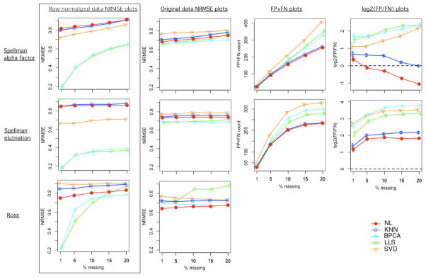
Simulation results for three datasets before/after row-wise mean removal. The datasets (labeled on the left side) are in rows and the type of results (labeled on top) are in columns. Error bars represent standard errors. The testing results (columns 3 and 4) were generated from the non-normalized data. The testing results for the Ross data are reported in Figure 2.

In order to make a comparison, we downloaded the raw data (original log-ratios) from the Stanford Microarray Database [30], and assembled the raw data matrix. When a gene was represented by more than one probes on the array, the mean of log ratios was taken to obtain a single reading. We then took the genes that were included in the simulation study with normalized data. Due to small differences in missing patterns, the numbers of genes were slightly different from the normalized data (Table 2). Using the non-normalized log ratios, we conducted another simulation study (parameters listed in Table 2). The results showed that with non-normalized data, although LLS and BPCA still led in performance in NRMSE, the difference between the methods was drastically smaller (Fig. 3, compare column 2 with column 1). To prove the point from the other end, we conducted another simulation using the NCI60 data. To introduce a dependency that is at similar level as the cell cycle data, we partitioned the NCI60 data matrix into three equal-sized sub-matrices, by selecting three groups of continuous columns – columns 1~20, 21~40, and 41~60. Within every sub-matrix, we conducted row-wise mean removal. Then we subjected the whole matrix to the mask-impute simulation procedure. The simulation yielded a dramatic decreases in the NRMSE from LLS and BPCA (Fig 3, row 3). Comparatively, the SVD method, although utilizing global dependency, did not make as much artificial gains when the data was row-normalized. This is because although the last three eigen values were driven to zero by row-normalization, the relative scale of the larger eigen values didn’t change much. The SVD method largely relies on the first several singular vectors, which prevented it from taking advantage of the perfect dependency created by row-wise mean removal. Based on these results, we can see that the impact of row-wise mean removal on the NRMSE results could be substantial. In addition to influencing the performance estimations in simulation studies, normalization can also impact real data analysis, in which we often resort to cross-validation using the complete portion of the data to select the method and parameter settings. The same artifact as detailed above could influence the choice of method and parameter settings, if the data is subjected to row-wise mean removal before the cross-validation.

Although LLS and BPCA didn’t show as much advantage using the original data, they still led in the performance as judged by NRMSE. This is expected because the cell-cycle arrays contain strong between-array dependencies [1]. We further explored whether the better NRMSE results translated to better testing results. Here we used the Fisher’s exact g test to find periodic behaviors in the genes, because the Spellman experiment was designed to find cell cycle-related genes. The FDR cutoff of 0.2 was used, which yielded ~10% significant genes in both datasets (Supporting Table 1). NL and KNN showed a clear lead in FP+FN counts despite they trailed in NRMSE results. Again NL was the most conservative method in terms of FP/FN ratio, though for the elutriation dataset all method yielded many more false positives than false negatives (Fig. 3, column 4).

To better understand why NL tended to be more conservative in terms of FP/FN ratio, we selected one of the scenarios, 10% missing in the Halbeisen dataset, for further examination. We repeated the mask-impute process 16 times and recorded the test p-values for all the genes. We then compared the test p-values after imputation against the complete-data p-values. For the NL method, 46.2% of the test p-values after imputation were smaller than the corresponding p-values from the complete data, while for all the other methods, over 50% of the test p-values after imputation were smaller than the corresponding p-values from the complete data (KNN: 52.6%, BPCA: 54.4%; LLS: 53.2%; SVD: 55.8%). Given that most of the genes were insignificant in the complete data, the tendency of the methods to decrease the p-values, even slightly, made a lot of false positives. NL was conservative in the sense that on average it tends to decrease the significance of a gene, albeit slightly, when imputation is done.

In summary, the non-linear imputation method based on SCOL and kernel smoother showed strong performance in the imputation of missing data, especially when judged by the impact on the statistical testing results. Aside from generating lower FP+FN counts, its property of being conservative in terms of FP/FN ratio is desirable, as controlling false discovery rate is a key concern when conducting tests using high-throughput data.

References

- 1.Brock GN, Shaffer JR, Blakesley RE, et al. Which missing value imputation method to use in expression profiles: a comparative study and two selection schemes. BMC Bioinformatics. 2008;9:12. doi: 10.1186/1471-2105-9-12. [DOI] [PMC free article] [PubMed] [Google Scholar]
- 2.Troyanskaya O, Cantor M, Sherlock G, et al. Missing value estimation methods for DNA microarrays. Bioinformatics. 2001 Jun;17(6):520–5. doi: 10.1093/bioinformatics/17.6.520. [DOI] [PubMed] [Google Scholar]
- 3.Bo TH, Dysvik B, Jonassen I. LSimpute: accurate estimation of missing values in microarray data with least squares methods. Nucleic Acids Res. 2004;32(3):e34. doi: 10.1093/nar/gnh026. [DOI] [PMC free article] [PubMed] [Google Scholar]
- 4.Yoon D, Lee EK, Park T. Robust imputation method for missing values in microarray data. BMC Bioinformatics. 2007;8(Suppl 2):S6. doi: 10.1186/1471-2105-8-S2-S6. [DOI] [PMC free article] [PubMed] [Google Scholar]
- 5.Kim H, Golub GH, Park H. Missing value estimation for DNA microarray gene expression data: local least squares imputation. Bioinformatics. 2005 Jan 15;21(2):187–98. doi: 10.1093/bioinformatics/bth499. [DOI] [PubMed] [Google Scholar]
- 6.Wong DS, Wong FK, Wood GR. A multi-stage approach to clustering and imputation of gene expression profiles. Bioinformatics. 2007 Apr 15;23(8):998–1005. doi: 10.1093/bioinformatics/btm053. [DOI] [PubMed] [Google Scholar]
- 7.Oba S, Sato MA, Takemasa I, et al. A Bayesian missing value estimation method for gene expression profile data. Bioinformatics. 2003 Nov 1;19(16):2088–96. doi: 10.1093/bioinformatics/btg287. [DOI] [PubMed] [Google Scholar]
- 8.Wang X, Li A, Jiang Z, et al. Missing value estimation for DNA microarray gene expression data by Support Vector Regression imputation and orthogonal coding scheme. BMC Bioinformatics. 2006;7:32. doi: 10.1186/1471-2105-7-32. [DOI] [PMC free article] [PubMed] [Google Scholar]
- 9.Jornsten R, Wang HY, Welsh WJ, et al. DNA microarray data imputation and significance analysis of differential expression. Bioinformatics. 2005 Nov 15;21(22):4155–61. doi: 10.1093/bioinformatics/bti638. [DOI] [PubMed] [Google Scholar]
- 10.Sehgal MS, Gondal I, Dooley LS. Collateral missing value imputation: a new robust missing value estimation algorithm for microarray data. Bioinformatics. 2005 May 15;21(10):2417–23. doi: 10.1093/bioinformatics/bti345. [DOI] [PubMed] [Google Scholar]
- 11.Sehgal MS, Gondal I, Dooley LS, et al. Ameliorative missing value imputation for robust biological knowledge inference. J Biomed Inform. 2008 Aug;41(4):499–514. doi: 10.1016/j.jbi.2007.10.005. [DOI] [PubMed] [Google Scholar]
- 12.Jornsten R, Ouyang M, Wang HY. A meta-data based method for DNA microarray imputation. BMC Bioinformatics. 2007;8:109. doi: 10.1186/1471-2105-8-109. [DOI] [PMC free article] [PubMed] [Google Scholar]
- 13.Tuikkala J, Elo L, Nevalainen OS, et al. Improving missing value estimation in microarray data with gene ontology. Bioinformatics. 2006 Mar 1;22(5):566–72. doi: 10.1093/bioinformatics/btk019. [DOI] [PubMed] [Google Scholar]
- 14.Gan X, Liew AW, Yan H. Microarray missing data imputation based on a set theoretic framework and biological knowledge. Nucleic Acids Res. 2006;34(5):1608–19. doi: 10.1093/nar/gkl047. [DOI] [PMC free article] [PubMed] [Google Scholar]
- 15.Xiang Q, Dai X, Deng Y, et al. Missing value imputation for microarray gene expression data using histone acetylation information. BMC Bioinformatics. 2008;9:252. doi: 10.1186/1471-2105-9-252. [DOI] [PMC free article] [PubMed] [Google Scholar]
- 16.Li KC, Liu CT, Sun W, et al. A system for enhancing genome-wide coexpression dynamics study. Proc Natl Acad Sci U S A. 2004 Nov 2;101(44):15561–6. doi: 10.1073/pnas.0402962101. [DOI] [PMC free article] [PubMed] [Google Scholar]
- 17.Suzuki T, Sugiyama M, Kanamori T, et al. Mutual information estimation reveals global associations between stimuli and biological processes. BMC Bioinformatics. 2009;10(Suppl 1):S52. doi: 10.1186/1471-2105-10-S1-S52. [DOI] [PMC free article] [PubMed] [Google Scholar]
- 18.Luo W, Hankenson KD, Woolf PJ. Learning transcriptional regulatory networks from high throughput gene expression data using continuous three-way mutual information. BMC Bioinformatics. 2008;9:467. doi: 10.1186/1471-2105-9-467. [DOI] [PMC free article] [PubMed] [Google Scholar]
- 19.Meyer PE, Lafitte F, Bontempi G. minet: A R/Bioconductor package for inferring large transcriptional networks using mutual information. BMC Bioinformatics. 2008;9:461. doi: 10.1186/1471-2105-9-461. [DOI] [PMC free article] [PubMed] [Google Scholar]
- 20.Zhou X, Wang X, Dougherty ER. Missing-value estimation using linear and non-linear regression with Bayesian gene selection. Bioinformatics. 2003 Nov 22;19(17):2302–7. doi: 10.1093/bioinformatics/btg323. [DOI] [PubMed] [Google Scholar]
- 21.Alizadeh AA, Eisen MB, Davis RE, et al. Distinct types of diffuse large B-cell lymphoma identified by gene expression profiling. Nature. 2000 Feb 3;403(6769):503–11. doi: 10.1038/35000501. [DOI] [PubMed] [Google Scholar]
- 22.Halbeisen RE, Gerber AP. Stress-Dependent Coordination of Transcriptome and Translatome in Yeast. PLoS Biol. 2009 May 5;7(5):e105. doi: 10.1371/journal.pbio.1000105. [DOI] [PMC free article] [PubMed] [Google Scholar]
- 23.Ross DT, Scherf U, Eisen MB, et al. Systematic variation in gene expression patterns in human cancer cell lines. Nat Genet. 2000 Mar;24(3):227–35. doi: 10.1038/73432. [DOI] [PubMed] [Google Scholar]
- 24.“http://0-www.ncbi.nlm.nih.gov.millennium.unicatt.it/projects/geo/query/acc.cgi?acc=GSE19119.”
- 25.Spellman PT, Sherlock G, Zhang MQ, et al. Comprehensive identification of cell cycle-regulated genes of the yeast Saccharomyces cerevisiae by microarray hybridization. Mol Biol Cell. 1998 Dec;9(12):3273–97. doi: 10.1091/mbc.9.12.3273. [DOI] [PMC free article] [PubMed] [Google Scholar]
- 26.Li KC, Yan M, Yuan SS. A simple statistical model for depicting the cdc15-synchronized yeast cell-cycle regulated gene expression data. Statistica Sinica. 2002 Jan;12(1):141–158. [Google Scholar]
- 27.Stacklies W, Redestig H, Scholz M, et al. pcaMethods--a bioconductor package providing PCA methods for incomplete data. Bioinformatics. 2007 May 1;23(9):1164–7. doi: 10.1093/bioinformatics/btm069. [DOI] [PubMed] [Google Scholar]
- 28.Storey JD, Tibshirani R. Statistical significance for genomewide studies. Proc Natl Acad Sci U S A. 2003 Aug 5;100(16):9440–5. doi: 10.1073/pnas.1530509100. [DOI] [PMC free article] [PubMed] [Google Scholar]
- 29.Wichert S, Fokianos K, Strimmer K. Identifying periodically expressed transcripts in microarray time series data. Bioinformatics. 2004 Jan 1;20(1):5–20. doi: 10.1093/bioinformatics/btg364. [DOI] [PubMed] [Google Scholar]
- 30.Demeter J, Beauheim C, Gollub J, et al. The Stanford Microarray Database: implementation of new analysis tools and open source release of software. Nucleic Acids Res. 2007 Jan;35(Database issue):D766–70. doi: 10.1093/nar/gkl1019. [DOI] [PMC free article] [PubMed] [Google Scholar]
Associated Data
This section collects any data citations, data availability statements, or supplementary materials included in this article.