Crowding: A cortical constraint on object recognition

Abstract

The external world is mapped retinotopically onto the primary visual cortex (V1). We show here that objects in the world, unless they are very dissimilar, can be recognized only if they are sufficiently separated in visual cortex: specifically, in V1, at least 6 mm apart in the radial direction (increasing eccentricity) or 1 mm apart in the circumferential direction (equal eccentricity). Objects closer together than this critical spacing are perceived as an unidentifiable jumble. This is called “crowding”. It severely limits visual processing, including speed of reading and searching. The conclusion about visual cortex rests on three findings. First, psychophysically, the necessary “critical” spacing, in the visual field, is proportional to (roughly half) the eccentricity of the objects. Second, the critical spacing is independent of the size and kind of object. Third, anatomically, the representation of the visual field on the cortical surface is such that position in V1 (and several other areas) is the logarithm of eccentricity in the visual field. Furthermore, we show that much of this can be accounted for by supposing that each “combining field”, defined by the critical spacing measurements, is implemented by a fixed number of cortical neurons.

Introduction

Although the conclusion of this review is about the brain physiology of object recognition, most of the research that led there was psychophysical study of acuity and reading. The link is new and surprising.

In the peripheral visual field, objects that would each be identifiable on their own become impossible to recognize when presented close together (Fig. 1). For each place (and direction) in the visual field there is a critical spacing (center to center) that must be exceeded for unimpaired recognition. Objects closer together than this critical spacing are perceived as an unidentifiable jumble. This is crowding. It severely limits visual processing, including speed of reading and searching.

Figure 1.

Crowding. While fixating the (red) minus, it is easy to identify the isolated letter on the left, but impossible to identify the middle letter on the right. The flankers, “a” and “e,” spoil recognition of the target. Fixating the (green) plus, it is easy to identify the r on the right. Reducing the eccentricity of the target reduces your critical spacing, which relieves crowding. Reprinted from [19].

Crowding, today, can be appreciated as a key fact about how people visually recognize objects. Object recognition has been studied intensely for a long time as a computational problem to which human visual perception provides a solution [4,5]. However, from its discovery until recently, crowding has been studied entirely outside of the research effort explicitly directed at object recognition. Today’s books on object recognition are including crowding for the first time[6]. For most of its history, crowding has been studied as a phenomenon of acuity and reading.

While it is obvious that vision is a complex function with many important parameters of performance, the variation of vision among people has always been, and is still, characterized predominantly by one number: acuity. Acuity is the threshold size for recognizing an object, typically a letter.

The familiar acuity chartused today, hardly changed from Snellen’s original [7], is designed to measure single-letter acuity. With that purpose, the letters are widely spaced, with a center-to-center spacing of about twice the letter size. This works well in normal observers viewing directly. That is, the acuity of normal observers is unaffected by the presence or absence of the letters surrounding the directly-viewed target letter. However, that two-letter spacing is not wide enough for strabismic amblyopes. Their measured acuity improves substantially if the surrounding letters are removed (by using a piece of paper with a hole in it to isolate the target letter). It turns out that the same is true for normal observers viewing peripherally, which is relevant to measuring acuity of patients with central field loss (e.g. macular degeneration) [8,9].

For Plato [10] and essentially everyone since, until recently, it seemed obvious that single-letter acuity accounted for the sharp decline in reading speed that occurs when a book is held too far away. However, increasing viewing distance, by moving the book farther away, confounds the effects of size and spacing. Repeating the experiment with text specially printed with extra-wide letter spacing reveals that under normal reading conditions the maximum distance of the book for fast reading is determined by letter spacing, not size [9]. If the spacing is wider, we can read quickly from farther.

Around 1900, it was discovered that reading consists of a series of eye fixations (four per second) rather than a continuous glide along the line of text [11]. It was natural to suppose that what the observer could take in from each fixation would be limited by his or her visual span. Visual span is the number of characters in a line of text that an observer can identify without moving his or her eyes. (This is not trivial because the fixations of reading are brief, 250 ms, but the visual span is usually measured with unlimited viewing time.) In fact, this simple model (reading speed proportional to visual span) accounts well for the effect of most visual variables on reading speed [12].

Visual span has long been a popular explanation for speed of reading and searching, but, until recently, only Woodworth [13] and Bouma [1] insisted that the visual span is limited by crowding (letter spacing), not acuity (letter size) [14].

This historical review of the origins of the idea of critical spacing has set the stage for our logical argument, which uses the critical spacing idea but is independent of its history. Three findings together yield a strong conclusion about the architecture of cortical processing in visual object recognition.

1. Critical spacing: Bouma’s proportionality constant

Wishing to understand how “lateral interaction” would limit how many letters a person reading can pick up in each fixation, Bouma measured the critical spacing for letter identification (a target letter between two flanking letters) as a function of eccentricity. He discovered that the critical spacing Δϕ is proportional to eccentricity ϕ,

$$\mathrm{\Delta }\varphi =b\varphi ,$$ (1)

where b is now called Bouma’s constant [1,14]. Bouma originally estimated that b is “roughly” 0.5 [1], and later refined this to about 0.4. He reported this result only for letters and only at one letter size. (More extensive measurements appear in Fig. 2.) However, Eq. 1, which looks so innocent, is a breakthrough. It represents his finding that the critical spacing varies enormously with position in the visual field, rather than being determined by object size.

Figure 2.

Critical spacing. The axes indicate position in the visual field, relative to the fixation point (grey “+” in upper left). In the upper right, also gray, we show a target letter between two symmetrically arranged flankers. The colored contour lines trace out the center-to-center target-to-flanker spacing the observer required to achieve 80% correct identification of the target letter. At each eccentricity, the black, red, and green curves represent different letter sizes. The results show that the critical spacing is proportional to radial eccentricity and independent of letter size. The symmetry of the plots results from the symmetry of the stimulus, which always had symmetrically opposed flankers. Each measured critical spacing is plotted as two opposing points. This is similar to the earlier measurements of Toet and Levi [3], but including several letter sizes. The anisotropy of critical spacing (radial over circumferential) is about 1.5 for this observer; Toet and Levi report an average of 2 for six observers, with large variations among observers. Letter sizes are 0.3, 0.43, and 0.55 deg at 5° and 6° ecc.; 0.43, 0.55, and 0.83 deg at 7.8° ecc.; 0.53, 0.83, and 1.2 deg at 12° ecc.; and 0.83, 1.2, and 1.5 at 13° ecc. Reprinted from [14].

Much of our daily visual experience is very nearly scale-invariant. We readily recognize letters and friends over a nearly thousand-fold range of size (in deg of visual angle). This led practically everyone to suppose that visual object recognition is scale invariant, though, in fact, the processing is scale-dependent [15,16]. Similarly, it has long been known that acuity is worse at more peripheral locations in the visual field, but it has been supposed that position in the visual field has little or no effect on the identifiability of objects that are big enough to exceed the acuity limit.

Bouma’s proportionality (Eq. 1) turns this conventional wisdom on its head. It identifies spacing, not size, as the key parameter, and it is determined by position in the visual field, not size of the objects.

2. Generality: the Bouma law

Interest in crowding has grown and grown to reach its present height [17–19]. It was important to learn that critical spacing (center to center) is independent of letter size [20–23]. Critical spacing has been measured for a wide range of tasks and objects. Eq. 1 holds up well. Extra terms have been added to the equation to fit data at very small and large eccentricities [3,14]. It is not surprising that the value of Bouma’s proportionality constant varies among studies that use different tasks and criteria for critical spacing [19].

Flanking objects that are less similar to the target produce less impairment of identification. However, studies that have disentangled the amplitude of crowding from spatial extent consistently find that similarity of the flankers to the target only affects the amplitude, not the spatial extent, of crowding [19,21,24,25].

Thus it seems that critical spacing (more precisely, the spatial extent of crowding) depends only on the location in the visual field (and direction from target to flanker), independent of object and size. This is demonstrated in Fig. 3.

Figure 3.

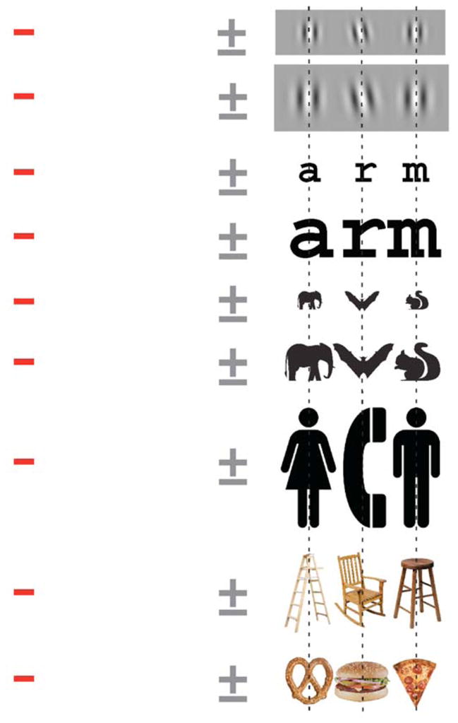
Critical spacing is independent of object and size. Fixating on the (red) minus, you will be unable to identify the middle object in each row, unless you isolate it by hiding the flanking objects with your fingers (or two pencils). Grating patches, like those in the top two rows, are often taken to be one-feature objects. In the first row, is the middle grating vertical or tilted? The ± is our estimate of the fixation point where you can just barely identify the target (Eq. 1 with b = 0.4). You can assess the accuracy of this threshold estimate by noting that the task is easy when you fixate to the right of the ±, and hard at the left. Critical spacing depends solely on position (and direction), in the visual field, which does not vary among rows in this demonstration. Note that halving object size has no effect on critical spacing. Critical spacing is independent of spatial frequency [21,61]. Reprinted, with modifications, from [19]. [Original sources: The gratings were created in MATLAB. The letters are in the Courier font. The animal silhouettes are in our Animals font, which is available for research purposes. The men, women, and telephone signs are from aiga.com [62]. The ladder is licensed from and copyright Stockbyte. The rocking chair is copyright 2008 Jupiter Images Corporation. In the following credits, we use the convention (Photographer/Name of collection/Source). The stool (C Squared Studios/Photodisc/Gettylmages), pretzel (Steve Wisbauer/Photodisc/Getty Images), hamburger (Ryan McVay/Photodisc/Getty Images), and pizza (Raimund Koch/Riser/Getty Images) are from Getty Images.]

3. Brain mapping

Independent of the psychophysical work on crowding, a succession of neuroscientists has used various techniques to produce ever-better maps describing the retinotopic correspondence between object position in the visual field and location of the response on the cortical surface in monkey [26–30] and man [2,31–39]. To a good approximation, in V1, and several other areas of human visual cortex, position d on the cortical surface of the response is the logarithm of the object’s eccentricity ϕ in the visual field,

$$d=\frac{log\varphi }{\beta }-\alpha ,$$ (2)

where α and β are empirical constants, unique to each visual area [2]. β is 0.06/mm for V1, 0.05/mm for V2, 0.05/mm for V3, 0.04/mm for LO1, 0.06/mm for LO2, and 0.05/mm for hV4 [2]. (Virtues and limitations of this logarithmic approximation are discussed in [29,40]. It requires modification to fit the smallest and largest eccentricies.)

Conclusion

Because of the logarithmic mapping (Eq. 2), a spacing Δϕ at the visual field that is proportional to eccentricity (Eq. 1) results in a fixed spacing Δd at the cortex,

$$\mathrm{\Delta }d=d_{\varphi +b\varphi }-d_{\varphi }=log(1+b)/\beta .$$ (3)

Taking b = 0.4, as in Fig. 3, and the value of β for V1, we find that Δd is 6 mm. Thus the logarithmic transformation of the proportional critical spacing at the visual field results in a fixed critical spacing at the cortex — 6 mm at V1 —independent of eccentricity [19,41,42]. (This is consistent with the estimated 6 mm range of dichoptic interactions in the region of V1 corresponding to the blindspot [43].) Up to this point, we have supposed that the objects are spaced radially (increasing eccentricity).

Anisotropy

A similar conclusion can be drawn for circumferential spacing of objects (equal eccentricity), but the critical spacing is much smaller — 1 mm at V1 — independent of eccentricity. Psychophysically, circumferential critical spacing is roughly half the radial critical spacing, with much variation within and across individuals [3]. Brain imaging finds anisotropy in the cortical magnification factor. In V1, Larsson and Heeger find itto be 1/3 as large in the circumferential as in the radial direction [2]. (Others report less anisotropy of cortical magnification, especially near the horizontal meridian, in monkey [44,45] and man [39].) At V1, these two factors make the circumferential critical spacing (1/2)x(1/3) = 1/6 of that in the radial direction, that is, 1 mm.

Other areas

The same conclusion applies to each of the logarithmically mapped visual areas, with differentvalues radially and circumferentially. The anisotropy is even more pronounced in higher-tier visual areas [2]. To recognize an object, the brain must combine its features. Perhaps one of these cortical areas combines features over the critical spacing [2,42,46–55].

The great anisotropy of critical spacing at the cortex surprised us, and we have no explanation for it, but it is not paradoxical, as there is no strong reason to expect isotropy. The strongest argument that we can make for invariant critical spacing at the cortex applies to the areal cortical magnification factor (mm² per deg²), the product of the radial and circumferential cortical magnification factors. The areal magnification is less variable than the linear magnification [30]. Let us call the area around the target circumscribed by the critical spacing in every direction (i.e. the ellipses in Fig. 2) the “combining field,” which corresponds to the older terms “association field,” “perceptual hypercolumn,” and “isolation field” [23,41,56]. Suppose that a certain fixed number of cortical neurons is required to do the computation (combining of features) that is associated with each combining field. Further suppose a fixed overlap factor of combining fields (the average number of fields that include any given point). The density of cortical neurons (per mm²) in visual cortex seems to be fixed, stable across individuals and species [57,58], so a fixed number of neurons will occupy a fixed area a. The large variations in brain size (and size of each visual area), within and across species, imply that smaller brains have fewer neurons and provide fewer combining fields, which would have to be larger (larger critical spacing) to provide the same coverage (see Appendix). Thus it would be interesting to measure critical spacing across species that have different brain size. Similarly, within a species, especially man, it would be interesting to look for correlation, across individuals, of critical spacing (measured psychophysically) and areal cortical magnification (measured, e.g., by fMRI).

We have concluded, firstly, that, for object recognition, there is a fixed critical spacing, in mm, for each of the logarithmically mapped visual areas (with different values radially and circumferentially), independent of the object’s kind, size and location. Secondly, we have no explanation for the radial-circumferential anisotropy, but if we embrace it as an empirical fact, then assuming that a fixed number of neurons implement each combining field provides a plausible model for the critical spacing results, and predicts a testable inverse relation between brain size and critical spacing at the visual field.

Symbols

b

Bouma’s proportionality constant for Eq. 1. “Roughly 0.5” [1]

ϕ

eccentricity (in deg) in the visual field [1]

Δϕ

critical spacing (in deg) at the visual field

d

position (in mm) on the cortical surface

Δd

critical spacing (in mm) on the cortical surface

αand β

here correspond to the Larsson & Heeger parameters a and b in Fig. 5 of [2]

η

anisotropy of crowding, the ratio of radial over circumferential critical spacing. About 2 [3]

a

area (mm²) of cortex occupied by the set of neurons that implement one combining field

A

area (in mm²) of cortex available

N

number of combining fields that can be implemented by an area A of cortex

o

overlap factor. The number of combining fields that include any given point in the visual field

Appendix: Brain size and critical spacing

Here we show that supposing that a fixed area of cortex is devoted to each combining field predicts that critical spacing will track changes in brain size. Specifically, changes in area of the cortex will produce inversely proportional changes in b log(1+b), where b is Bouma’s constant, which determines the critical spacing Δϕ = bϕ.

For eccentricity, we take a section of a cortical map (e.g. V1) that is accurately logarithmic, using only eccentricities in the range ϕ_min < ϕ < ϕ_max, with bounds, e.g., ϕ_min = 1° and ϕ_max = 5°. For polar angle, we take the whole semicircular range of one hemisphere’s map, 0 < ψ < 180°. The critical spacing radially, outwards, from target to flanker is Δϕ = bϕ. Circumferentially the critical spacing is b′ϕ, where we define b′ = b/η, and η is the anisotropy (η ≈ 2) of the critical spacing (ratio of radial to circumferential). The ratio of eccentricities of a critically spaced flanker (outward, radially) and target is (1+b)ϕ/ϕ = 1+b. We suppose that that the radial critical spacing inward is in the same proportion, so that the ratio of greatest to smallest eccentricity of the combining field is (1+b)². Circumferentially the critical spacing, expressed as polar angle, is Δψ = (180/π)b′ϕ/ϕ = (180/π)b/η. The polar extent of the field is 2Δψ. If we “tile” the visual field (within the specified bounds) with abutting fields then at any given polar angle the number n of abutting fields radially from ϕ_min to ϕ_max will be

$$n=log({\varphi }_{max}/{\varphi }_{min})/log[{(1+b)}^2]$$ (A1)

At any given eccentricity, number n′ of fields abutting circumferentially will be

$$n^{\prime }=180/(2\mathrm{\Delta }\psi )$$ (A2)

$$=\pi /(2b/\eta ).$$ (A3)

The total number of fields tiling the visual field will be their product, n′n. Allowing for an overlap factor of o, the total number N of fields needed to service the specified visual area is

$$N={on}^{\prime }n.$$ (A4)

We have supposed that the neurons required to implement a combining field occupy an area a (in mm²). Let the section of cortex have area A (in mm²). This provides enough neurons to make N combining fields,

$$N=A/a.$$ (A5)

Putting together our two equations for N, we have

$${on}^{\prime }n=A/a,$$ (A6)

which expands to

$$o[\pi /(2b/\eta )]log({\varphi }_{max}/{\varphi }_{min})/[2log(1+b)]=A/a,$$ (A7)

which we can rearrange to

$$blog(1+b)=A^{-1}ao\pi \eta log({\varphi }_{max}/{\varphi }_{min})/4.$$ (A8)

On the left, we have an expression in b, Bouma’s constant. Note that for small b, log(1+b) is approximately b. Thus the left-hand expression is roughly b². On the right, the cortical area A is the most variable quantity, known to vary two-fold within a species. The area a is our invention, the area occupied by the number of neurons required to implement a combining field. We suppose that this is constant for a given region of the visual cortex within a species, but would depend on the number of dimensions (features) that are being combined [59,60], which differs among regions of the cortex and may differ between homologous regions in different species. The remaining terms—overlap factor o and anisotropy η—seem unlikely to change much. Thus, supposing that a fixed number of cortical neurons implements each combining field predicts that changes in area of the cortex will produce inversely proportional changes in b log(1+b), where b is Bouma’s constant, determining the critical spacing Δϕ = bϕ. QED.

References

Papers of special or outstanding interest are flagged * or **.
[The reference list below is dynamically updated by Endnote, so I am writing out my reference comments separately, here at the top. They should be merged in producing the final print version. -denis]
- 1**.Bouma H. Interaction effects in parafoveal letter recognition. Nature. 1970;226:177–178. doi: 10.1038/226177a0. In two pages, Bouma introduced the idea of critical spacing, presented measurements as a function of eccentricity, and noted that it is roughly half the eccentricity. This was a breakthrough, counter to firmly established ideas that visibility depends on size (acuity) not spacing. [DOI] [PubMed] [Google Scholar]
- 2*.Larsson J, Heeger DJ. Two retinotopic visual areas in human lateral occipital cortex. J Neurosci. 2006;26:13128–13142. doi: 10.1523/JNEUROSCI.1657-06.2006. Beautiful fMRI measurements of retinotopy in six visual areas. Their exponential fit of eccentricity vs. cortical distance, ϕ =exp[β (d+α)], is equivalent to a logarithmic fit of cortical distance vs. eccentricity, d=(log ϕ)/β – α, which is our Eq. 2 above. [DOI] [PMC free article] [PubMed] [Google Scholar]
- 3*.Toet A, Levi DM. The two-dimensional shape of spatial interaction zones in the parafovea. Vision Res. 1992;32:1349–1357. doi: 10.1016/0042-6989(92)90227-a. A classic paper, it shows the importance of measuring thoroughly and systematically, not just a few points. Before this paper, one would have expected maps of critical spacing to be regular and symmetric, as in [63]. The Toet and Levi maps reveal unexpected variations and asymmetries in critical spacing, within and across observers. The variations in critical spacing remain unexplained, but suggest an organic rather than a crystalline process. [DOI] [PubMed] [Google Scholar]
- 4.Ullman S. High-level vision: object recognition and visual cognition. Cambridge, Mass: MIT Press; 2000. [Google Scholar]
- 5.Duda RO, Hart PE, Stork DG. Pattern classification. 2. New York: Wiley; 2001. [Google Scholar]
- 6.Strasburger H, Rentschler I. Pattern recognition in direct and indirect view. In: Osaka N, Rentschler I, Biederman I, editors. Object recognition, attention, and action. Springer; 2007. pp. 41–54. [Google Scholar]
- 7.Snellen H. Test-types for the determination of the acuteness of vision. London: Norgate and Williams; 1866. [Google Scholar]
- 8.Korte W. Uber die Gestaltauffassung im indirekten Sehen. Zeitschrift für Psychologie. 1923;93:17–82. [Google Scholar]
- 9.Levi DM, Song S, Pelli DG. Amblyopic reading is crowded. J Vis. 2007;7:21, 21–17. doi: 10.1167/7.2.21. [DOI] [PubMed] [Google Scholar]
- 10.Plato. Republic, 2, line 368d. Indianapolis: Hackett Publishing Co; 1992. [Google Scholar]
- 11.Huey EB. The psychology and pedagogy of reading. New York: Macmillan; 1908. [Google Scholar]
- 12*.Legge GE. Psychophysics of reading in normal and low vision. Mahwah, NJ: Erlbaum; 2007. This excellent book puts together all the literature on the psychophysics of reading, a substantial part of which is Legge’s own contributions. [Google Scholar]
- 13*.Woodworth RS. Experimental psychology. New York: Holt; 1938. p. 720. Presents demos to measure the reader’s visual span, showing that it is limited by letter spacing (crowding) not size (acuity) [Google Scholar]
- 14*.Pelli DG, Tillman KA, Freeman J, Su M, Berger TD, Majaj NJ. Crowding and eccentricity determine reading rate. J Vis. 2007;7:20, 21–36. doi: 10.1167/7.2.20. Joins together the contributions of Bouma (crowding) and Legge (visual span), working out the geometrical calculations in detail and presenting a great deal of empirical data showing that crowding does indeed determine the visual span and thus reading rate. [DOI] [PubMed] [Google Scholar]
- 15.Pelli DG. Close encounters-an artist shows that size affects shape. Science. 1999;285:844–846. doi: 10.1126/science.285.5429.844. [DOI] [PubMed] [Google Scholar]
- 16.Majaj NJ, Pelli DG, Kurshan P, Palomares M. The role of spatial frequency channels in letter identification. Vision Res. 2002;42:1165–1184. doi: 10.1016/s0042-6989(02)00045-7. [DOI] [PubMed] [Google Scholar]
- 17*.Levi DM. Crowding - an essential bottleneck for object recognition: A mini-review. Vision Res. 2008;48:635–354. doi: 10.1016/j.visres.2007.12.009. A broad review of current work and ideas in crowding. [DOI] [PMC free article] [PubMed] [Google Scholar]
- 18.Pelli DG, Cavanagh P, Desimone R, Tjan BS, Treisman AM. Crowding: Including illusory conjunctions, surround suppression, and attention. Journal of Vision. 2007;7(2i):1. doi: 10.1167/7.2.i. [DOI] [PubMed] [Google Scholar]
- 19*.Pelli DG, Tillman KA. The uncrowded window of object recognition. Nature Neuroscience. 2008 doi: 10.1038/nn.2187. in press. A review, complementing Levi’s, which focuses on the generality of Bouma’s critical spacing, and sketches the V1 argument that is the focus of the present review. [DOI] [PMC free article] [PubMed] [Google Scholar]
- 20.Strasburger H, Harvey LO, Jr, Rentschler I. Contrast thresholds for identification of numeric characters in direct and eccentric view. Percept Psychophys. 1991;49:495–508. doi: 10.3758/bf03212183. [DOI] [PubMed] [Google Scholar]
- 21*.Levi DM, Hariharan S, Klein SA. Suppressive and facilitatory spatial interactions in peripheral vision: peripheral crowding is neither size invariant nor simple contrast masking. J Vis. 2002;2:167–177. doi: 10.1167/2.2.3. A thoughtful piece with lots of data. Presents the idea of crowding as feature pooling over large distances. [DOI] [PubMed] [Google Scholar]
- 22.Tripathy SP, Cavanagh P. The extent of crowding in peripheral vision does not scale with target size. Vision Res. 2002;42:2357–2369. doi: 10.1016/s0042-6989(02)00197-9. [DOI] [PubMed] [Google Scholar]
- 23*.Pelli DG, Palomares M, Majaj NJ. Crowding is unlike ordinary masking: distinguishing feature integration from detection. J Vis. 2004;4:1136–1169. doi: 10.1167/4.12.12. This article helped create a wider awareness of crowding as a basic visual phenomenon. It proposed empirical tests to distinguish crowding from other kinds of masking. It reviewed the phenomenology of crowding, both in the literature and in a series of empirical studies of many relevant parameters. It showed that most of the papers on illusory conjunction were studying crowding. [DOI] [PubMed] [Google Scholar]
- 24.Andriessen JJ, Bouma H. Eccentric vision: adverse interactions between line segments. Vision Res. 1976;16:71–78. doi: 10.1016/0042-6989(76)90078-x. [DOI] [PubMed] [Google Scholar]
- 25.Wilkinson F, Wilson HR, Ellemberg D. Lateral interactions in peripherally viewed texture arrays. J Opt Soc Am A. 1997;14:2057–2068. doi: 10.1364/josaa.14.002057. [DOI] [PubMed] [Google Scholar]
- 26.Talbot SA, Marshall WH. Physiological studies on neural mechanisms of visual localization and discrimination. Am j Ophthal. 1941;24:1255–1264. [Google Scholar]
- 27.Daniel PM, Whitteridge D. The representation of the visual field on the cerebral cortex in monkeys. J Physiol. 1961;159:203–221. doi: 10.1113/jphysiol.1961.sp006803. [DOI] [PMC free article] [PubMed] [Google Scholar]
- 28.Hubel DH, Wiesel TN. Uniformity of monkey striate cortex: a parallel relationship between field size, scatter, and magnification factor. J Comp Neurol. 1974;158:295–305. doi: 10.1002/cne.901580305. [DOI] [PubMed] [Google Scholar]
- 29.Van Essen DC, Newsome WT, Maunsell JHR, Bixby JL. The projections from striate cortex (V1) to areas V2 and V3 in the macaque monkey: asymmetries, areal boundaries, and patchy connections. J Comp Neurol. 1986;244:451–480. doi: 10.1002/cne.902440405. [DOI] [PubMed] [Google Scholar]
- 30.Adams DL, Horton JC. A precise retinotopic map of primate striate cortex generated from the representation of angioscotomas. J Neurosci. 2003;23:3771–3789. doi: 10.1523/JNEUROSCI.23-09-03771.2003. [DOI] [PMC free article] [PubMed] [Google Scholar]
- 31.Inouye T. Die Sehstörungen bei Schussverletzungen der kortikalen Sehsphäre nach Beobachtungen an Verwundeten der letzten japanischen Kriege. Leipzig: Engelmann; 1909. [Google Scholar]
- 32.Holmes G, Lister WT. Disturbances of vision from cerebral lesions with special reference to the cortical representation of the macula. Brain. 1916;39:34. [PMC free article] [PubMed] [Google Scholar]
- 33.Penfield W, Jaspers H, McNaughton F. Epilepsy and the functional anatomy of the human brain. Boston: Little, Brown; 1954. [Google Scholar]
- 34.Cowey A, Rolls ET. Human cortical magnification factor and its relation to visual acuity. Exp Brain Res. 1974;21:447–454. doi: 10.1007/BF00237163. [DOI] [PubMed] [Google Scholar]
- 35.Fox PT, Miezin FM, Allman JM, Van Essen DC, Raichle ME. Retinotopic organization of human visual cortex mapped with positron-emission tomography. J Neurosci. 1987;7:913–922. doi: 10.1523/JNEUROSCI.07-03-00913.1987. [DOI] [PMC free article] [PubMed] [Google Scholar]
- 36.Sereno MI, Dale AM, Reppas JB, Kwong KK, Belliveau JW, Brady TJ, Rosen BR, Tootell RB. Borders of multiple visual areas in humans revealed by functional magnetic resonance imaging. Science. 1995;268:889–893. doi: 10.1126/science.7754376. [DOI] [PubMed] [Google Scholar]
- 37.DeYoe EA, Carman GJ, Bandettini P, Glickman S, Wieser J, Cox R, Miller D, Neitz J. Mapping striate and extrastriate visual areas in human cerebral cortex. Proc Natl Acad Sci USA. 1996;93:2382–2386. doi: 10.1073/pnas.93.6.2382. [DOI] [PMC free article] [PubMed] [Google Scholar]
- 38.Engel SA, Glover GH, Wandell BA. Retinotopic organization in human visual cortex and the spatial precision of functional MRI. Cereb Cortex. 1997;7:181–192. doi: 10.1093/cercor/7.2.181. [DOI] [PubMed] [Google Scholar]
- 39.Duncan RO, Boynton GM. Cortical magnification within human primary visual cortex correlates with acuity thresholds. Neuron. 2003;38:659–671. doi: 10.1016/s0896-6273(03)00265-4. [DOI] [PubMed] [Google Scholar]
- 40.Schwartz EL. Computational anatomy and functional architecture of striate cortex: a spatial mapping approach to perceptual coding. Vision Res. 1980;20:645–669. doi: 10.1016/0042-6989(80)90090-5. [DOI] [PubMed] [Google Scholar]
- 41*.Levi DM, Klein SA, Aitsebaomo AP. Vernier acuity, crowding and cortical magnification. Vision Res. 1985;25:963–977. doi: 10.1016/0042-6989(85)90207-x. Measured crowding for Vernier acuity and used estimates of the cortical magnification factor to conclude that “spatial interference occurred when the interline distance was less than a cortical distance of about 1 mm.” The spacing was horizontal in the lower visual field, so the 1 mm critical spacing was circumferential, consistent with what we find here. [DOI] [PubMed] [Google Scholar]
- 42*.Motter BC, Simoni DA. The roles of cortical image separation and size in active visual search performance. J Vis. 2007;7(6):1–15. doi: 10.1167/7.2.6. Measured eye position during visual search and found that search performance depends on distance, in cortical space, from target to nearest neighbor. [DOI] [PubMed] [Google Scholar]
- 43.Tripathy SP, Levi DM. Long-range dichoptic interactions in the human visual cortex in the region corresponding to the blind spot. Vision Res. 1994;34:1127–1138. doi: 10.1016/0042-6989(94)90295-x. [DOI] [PubMed] [Google Scholar]
- 44.Yang Z, Heeger DJ, Seidemann E. Rapid and precise retinotopic mapping of the visual cortex obtained by voltage-sensitive dye imaging in the behaving monkey. J Neurophysiol. 2007;98:1002–1014. doi: 10.1152/jn.00417.2007.. [DOI] [PMC free article] [PubMed] [Google Scholar]
- 45.Tootell RB, Switkes E, Silverman MS, Hamilton SL. Functional anatomy of macaque striate cortex. II. Retinotopic organization. J Neurosci. 1988;8:1531–1568. doi: 10.1523/JNEUROSCI.08-05-01531.1988. [DOI] [PMC free article] [PubMed] [Google Scholar]
- 46.Miller EK, Gochin PM, Gross CG. Suppression of visual responses of neuronsin inferior temporal cortex of the awake macaque by addition of a second stimulus. Brain Res. 1993;616:25–29. doi: 10.1016/0006-8993(93)90187-r. [DOI] [PubMed] [Google Scholar]
- 47.Logothetis NK, Sheinberg DL. Visual object recognition. Annu Rev Neurosci. 1996;19:577–621. doi: 10.1146/annurev.ne.19.030196.003045. [DOI] [PubMed] [Google Scholar]
- 48.Luck SJ, Chelazzi L, Hillyard SA, Desimone R. Neural mechanisms of spatial selective attention in areas V1, V2, and V4 of macaque visual cortex. J Neurophysiol. 1997;77:24–42. doi: 10.1152/jn.1997.77.1.24. [DOI] [PubMed] [Google Scholar]
- 49.Gallant JL, Connor CE, Van Essen DC. Neural activity in areas V1, V2 and V4 during free viewing of natural scenes compared to controlled viewing. Neuroreport. 1998;9:2153–2158. doi: 10.1097/00001756-199806220-00045. [DOI] [PubMed] [Google Scholar]
- 50.Motter BC. Crowding and object integration within the receptive field of V4 neurons. Journal of Vision. 2002;2:274. [Google Scholar]
- 51.Rolls ET, Aggelopoulos NC, Zheng F. The receptive fields of inferior temporal cortex neurons in natural scenes. J Neurosci. 2003;23:339–348. doi: 10.1523/JNEUROSCI.23-01-00339.2003. [DOI] [PMC free article] [PubMed] [Google Scholar]
- 52.Zoccolan D, Cox DD, DiCarlo JJ. Multiple object response normalization in monkey inferotemporal cortex. J Neurosci. 2005;25:8150–8164. doi: 10.1523/JNEUROSCI.2058-05.2005. [DOI] [PMC free article] [PubMed] [Google Scholar]
- 53.Rollenhagen JE, Olson CR. Low-frequency oscillations arising from competitive interactions between visual stimuli in macaque inferotemporal cortex. J Neurophysiol. 2005;94:3368–3387. doi: 10.1152/jn.00158.2005. [DOI] [PubMed] [Google Scholar]
- 54.Fallah M, Stoner GR, Reynolds JH. Stimulus-specific competitive selection in macaque extrastriate visual area V4. Proc Natl Acad Sci U S A. 2007;104:4165–4169. doi: 10.1073/pnas.0611722104. [DOI] [PMC free article] [PubMed] [Google Scholar]
- 55.Vinberg J, Grill-Spector K. Representation of shapes, edges, and surfaces across multiple cues in the human visual cortex. J Neurophysiol. 2008;99:1380–1393. doi: 10.1152/jn.01223.2007. [DOI] [PubMed] [Google Scholar]
- 56.Field DJ, Hayes A, Hess RF. Contour integration by the human visual system:evidence for a local “association field”. Vision Res. 1993;33:173–193. doi: 10.1016/0042-6989(93)90156-q. [DOI] [PubMed] [Google Scholar]
- 57.Rockel AJ, Hiorns RW, Powell TP. The basic uniformity in structure of the neocortex. Brain. 1980;103:221–244. doi: 10.1093/brain/103.2.221. [DOI] [PubMed] [Google Scholar]
- 58.Braitenberg V, Schüz A. Cortex: Statistics and Geometry of Neuronal Connectivity, Second Edition. Heidelberg, Germany: Springer Verlag; 1998. [Google Scholar]
- 59.Durbin R, Mitchison G. A dimension reduction framework for understanding cortical maps. Nature. 1990;343:644–647. doi: 10.1038/343644a0. [DOI] [PubMed] [Google Scholar]
- 60.Swindale NV. How different feature spaces maybe represented in cortical maps. Network. 2004;15:217–242. [PubMed] [Google Scholar]
- 61.Chung STL, Levi DM, Legge GE. Spatial-frequency and contrast properties of crowding. Vision Res. 2001;41:1833–1850. doi: 10.1016/s0042-6989(01)00071-2. [DOI] [PubMed] [Google Scholar]
- 62.AIGA. The complete study of passenger/pedestrian symbols developed by the American Institute of Graphic Arts for the US Department of Transportation. 2. New York: AIGA; 1993. Symbol signs. [Google Scholar]
- 63.Bouma H. Visual search and reading: eye movements and functional visual field: a tutorial review. In: Requin J, editor. Attention and performance, VII. Lawrence Erlbaum Associates; 1978. pp. 115–147. [Google Scholar]