Accounting for non-genetic factors by low-rank representation and sparse regression for eQTL mapping

Abstract

Motivation: Expression quantitative trait loci (eQTL) studies investigate how gene expression levels are affected by DNA variants. A major challenge in inferring eQTL is that a number of factors, such as unobserved covariates, experimental artifacts and unknown environmental perturbations, may confound the observed expression levels. This may both mask real associations and lead to spurious association findings.

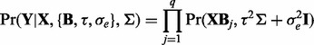
Results: In this article, we introduce a LOw-Rank representation to account for confounding factors and make use of Sparse regression for eQTL mapping (LORS). We integrate the low-rank representation and sparse regression into a unified framework, in which single-nucleotide polymorphisms and gene probes can be jointly analyzed. Given the two model parameters, our formulation is a convex optimization problem. We have developed an efficient algorithm to solve this problem and its convergence is guaranteed. We demonstrate its ability to account for non-genetic effects using simulation, and then apply it to two independent real datasets. Our results indicate that LORS is an effective tool to account for non-genetic effects. First, our detected associations show higher consistency between studies than recently proposed methods. Second, we have identified some new hotspots that can not be identified without accounting for non-genetic effects.

Availability: The software is available at: http://bioinformatics.med.yale.edu/software.aspx.

Contact: hongyu.zhao@yale.edu

Supplementary information: Supplementary data are available at Bioinformatics online.

1 INTRODUCTION

Nowadays both gene expression levels and hundreds of thousands of single-nucleotide polymorphisms (SNPs) can be measured by high-throughput technologies. This allows us to systematically explore the relationship between gene expression levels and genotypes: whether a gene is differentially expressed with different genotypes (or alleles) at a specific locus. The loci that are associated with gene expression levels are known as ‘expression quantitative trait loci’ (eQTL) (Li et al., 2012). Recently, a large number of eQTLs have been found in eQTL studies (Cookson et al., 2009). These findings provide insights on how gene expression levels are affected by specific genetic variants (Cheung and Spielman, 2009). They may further help to prioritize disease-associated loci and contribute to disease understanding (Nica and Dermitzakis, 2008).

An important issue in eQTL mapping is that a fairly large proportion of the measured gene expression variations may not be caused by genetic variants, but by some other factors, including cellular state (Alter et al., 2000), environmental factors (Gibson, 2008) and experimental conditions (Leek et al., 2010). A typical example is the batch effect, which may arise when sub-groups of samples were processed by different laboratories, different technicians or on different days. Because these factors are unrelated to genetic variants, we call them non-genetic factors in the rest of the article.

Some of the non-genetic effects can be directly measured. For example, when the batch information is available, the batch effects may be adjusted, e.g an empirical Bayes method named ‘Combat’ (Li and Rabinovic, 2007). However, in practice, non-genetic factors may not be directly and completely observable and thus remain hidden. For example, Pastinen et al. (2006) showed that cell culture conditions have an unnegligible influence on a large number of genes. Gagnon-Bartsch and Speed (2012) reported that a substantial within-batch effect exists in the Microarray Quality Control study (Shi et al., 2006). ‘Expression heterogeneity’ (EH) arises when these hidden factors are not taken into account in statistical analysis. Leek and Storey (2007) showed that EH not only leads to the reduction of statistical power but also spurious association signals in eQTL mapping.

Recently, capturing EH in gene expression studies has drawn the attention of researchers. Many methods have been proposed to infer the hidden factors by some forms of factor analysis, and adjust the inferred factors as if they were observed (Alter et al., 2000; Nielsen et al., 2002).

One well-known method that attempts to address these issues is the Surrogate Variable Analysis (SVA; Leek and Storey, 2007). It performs principal component analysis while taking genotypes into consideration and uses permutation to choose the number of principal components. Kang et al. (2008) proposed the intersample correlation emended (ICE) eQTL mapping method, in which a linear mixed model was introduced to model the hidden factors. When modeling EH, Kang et al. (2008) used the covariance matrix of the gene expression data as the EH covariance matrix in their ICE model. However, this estimate is inconsistent and thus reduces the power of eQTL mapping. Listgarten et al. (2010) introduced another linear mixed model, named ‘LMM-EH’, which corrected the inconsistency of the estimated EH covariance matrix. Once the latent covariance matrix has been estimated, LMM-EH can scan every gene-SNP pair. Alternatively, Stegle et al. (2010) jointly modeled SNPs, gene probes and hidden confounders into a Bayesian framework. Despite its greatly increased power in eQTL mapping, its heavy computational burden might limit its usage. Fusi et al. (2012) proposed another model named ‘PANAMA’ and borrowed some computational techniques from Gaussian process (Rasmussen and Williams, 2006) and further improved the performance of eQTL mapping. However, during the model optimization, PANAMA may be trapped in a local optimum because the optimization problem is not convex.

In this article, we introduce an alternative formulation to address this issue. We propose a LOw-Rank representation to account for non-genetic factors and make use of Sparse regression for eQTL mapping (LORS). We integrate the low-rank representation and sparse regression into a unified framework, in which SNPs and gene probes can be jointly analyzed. Given the two regularization parameters, the optimization of the model structure is a convex problem. We have developed an efficient algorithm to solve this convex problem and its convergence is guaranteed. We demonstrate its usefulness through its applications to both synthetic data and real data.

2 MODEL

Before introducing our formulation, we summarize the notations used in this article. We consider the following norms of a vector : the norm defined as ; the and the squared norms defined as 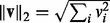and , respectively. We use the following three norms of a matrix : the Frobenius norm 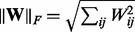, the nuclear norm 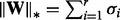, where are the singular values of and r is the rank of and the ‘elementwise’ norm .

Let be an matrix corresponding to a gene expression dataset, where n is the number of samples and q is the number of genes. Let be an matrix corresponding to a SNP dataset, where p is the number of SNPs. To model the relationship between and , we propose to decompose as:

(1)

where is the coefficient matrix, is a vector whose entries are all 1, is a matrix with being the j-th intercept and is a Gaussian random noise term with zero mean and variance , i.e. . Here we introduce in our model to account for the variations caused by a few hidden factors. This model implies that gene expression levels are influenced by genetic factors, non-genetic factors and random noises.

To make the decomposition (1) possible, we make the following assumptions:

• There are only a few hidden factors that may influence gene expression levels. Thus, is a low-rank matrix. Here, we also implicitly assume that the hidden factors have global effects rather than local effects.

• The gene expression level may only be affected by a small fraction of SNPs. This implies that the coefficient matrix should be sparse.

Based on these assumptions, we propose to solve the following optimization problem:

(2)

where is the elementwise norm defined before, r₀ and t₀ are some fixed constants. To make the minimization problem tractable, we relax the rank operator on with the nuclear norm, which has been proven to be an effective convex surrogate of the rank operator (Recht et al., 2010). Now we rewrite (2) in a Lagrange form

(3)

where is the nuclear norm of , ρ and λ are regularization parameters that control the sparsity of and the rank of , respectively. Now it is a convex optimization problem and can be solved efficiently.

Missing data are commonly encountered when analyzing gene expression data. Here we extend our basic model (3) in the following to handle missing data naturally.

Suppose we only observed a subset of entries in , indexed by . The unobserved entries are indexed by . Mathematically, we can define an orthogonal projection operator that projects a matrix onto the linear space of matrices supported by :

(4)

and is its complementary projection, i.e. (W) = W.

Because we want to find a sparse coefficient matrix and a low-rank matrix based on the observed data, we propose to solve the following optimization problem:

(5)

where the first term 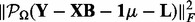is the sum of squared errors on the observed entries indexed by .

3 ALGORITHM

To solve the optimization problem (3) efficiently, we need the following lemma [the proof can be found in (Mazumder et al., 2010)]:

Lemma 1 —

Suppose matrix has rank r. The solution to the optimization problem

(6)

is given by where

(7)

is the Singular Value Decomposition (SVD) of , , and .

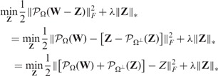
We adopt an alternating strategy to solve problem (3). For fixed and , the optimization problem becomes

(8)

By Lemma 1, we have a closed-form solution for :

(9)

For fixed , the optimization problem becomes

(10)

It can be further decomposed into q independent Lasso problems (Tibshirani, 1996):

(11)

where and are the j-th column of and , respectively. The Lasso problem can be solved efficiently by the coordinate descent algorithm (Friedman et al., 2007, 2010). Now we have Algorithm 1:

Algorithm 1 A fast algorithm to solve problem (3).

• Input: . Initialize , .

• Iterate until convergence:

  • -step: .
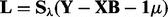  • -step: Solve q independent Lasso problems (11) by the coordinate descent algorithm.

• Output: , , .

So far we have developed the algorithm for solving problem (3). To derive an algorithm to solve optimization problem (5), we need the following lemma [its proof was given by (Mazumder et al., 2010)]:

Lemma 2 —

Soft-impute algorithm

(12)

By Lemma 1, the optimal value of the optimization problem (12) can be obtained via updating using

(13)

with an arbitrary initialization.

We also adopt the alternating strategy to solve (5). For fixed and , optimization problem (5) becomes

(14)

By Lemma 2 we have

(15)

For fixed , optimization problem (5) becomes

(16)

Again, this problem can be decomposed into q independent Lasso problems as follows:

(17)

Now we have Algorithm 2:

Algorithm 2 A fast algorithm to solve problem (5).

• Input: . Initialize , .

• Iterate until convergence:

  • -step: iteratively update using (15).
  • -step: Solve q independent Lasso problems (17) using the coordinate descent algorithm.

• Output: , , .

The convergence analysis of our algorithms and the CPU timings are provided in the Supplementary Document.

4 PARAMETER TUNING

We have two parameters that need to be tuned in our models. Here we propose a cross-validation-like strategy to select these two parameters. The idea is as follows: Let be the index of the observed entries of . We randomly divide into training entries and testing entries : and . The sizes of and are roughly the same. We may solve problem (5) on a grid of () values on the training data:

(18)

Then we evaluate the prediction error (19) on the testing data

(19)

where we write , and as , and to emphasize that , and depend on the parameters ρ and λ. We can then choose the parameter setting , which minimizes the prediction error (19).

However, searching for two parameters on a grid of values may be too computationally expensive when dealing with large datasets. Instead, we search a good λ value with fixing and then perform a one dimensional search on a sequence of ρ values. In our implementation, we first set the maximum rank of , denoted as , equal to . Then, we start from a large , which equals to the second largest singular value of matrix . After solving

(20)

if , we reduce λ by a factor and repeatedly solve (20) until . Using warm-start, this sequential optimization is efficient (Mazumder et al., 2010).

Then we choose a λ value, which minimizes the prediction error

(21)

Let be the value corresponding to the minimal prediction error (21). Now we can perform a one dimensional search for a good value for ρ. We generate a sequence of ρ values with length equally decreasing from to on the log scale, where is the smallest ρ value such that all entries of are zero. Typically, we set and . For each ρ value, we solve

(22)

and evaluate the prediction error:

(23)

Then we choose the ρ value corresponding to the minimal prediction error (23). Now we can solve model (5) using () as regularization parameters, and obtain a sparse matrix and a low rank matrix .

5 DISCUSSION

5.1 Relationship between our method and other methods

To our knowledge, LMM-EH (Listgarten et al., 2010) proposed the first framework, where multiple gene expression levels and confounder effects can be jointly analyzed in eQTL studies. For the j-th gene expression level in the LMM-EH model, it assumes the following structure:

(24)

where are the expression and SNP data matrices, respectively. Here denotes Gaussian noise, i.e. , and denotes a random effect, i.e. , where τ is a scalar and . Assuming the independence among , and integrate out and , we arrive at the following form:

(25)

LMM-EH adopts the following strategy to estimate the covariance matrix and other model parameters :

• First, it estimates from the null model, which does not include any SNPs, denoted as (Kang et al., 2008, 2010; Lippert et al., 2011).

• Second, using in model (24) as a known covariance and estimate for all gene-SNP pairs (one gene versus one SNPs at a time).

PANAMA extends LMM-EH and allows joint analysis of all SNPs (Fusi et al., 2012). Specifically, PANAMA models the relationship between gene expression levels and SNPs as follows:

(26)

here is the intercept, and are the corresponding coefficients representing the effects of SNPs and hidden factors . PANAMA assigns independent Gaussian priors for and :

(27)

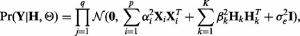
where K is the number of hidden factors. Assuming … , q are independent and integrating out and , the model becomes

(28)

where the intercept term is dropped for notation convenience and . In principle, parameter estimation in (28) can be done by borrowing some computational tricks from Gaussian process model optimization (Rasmussen and Williams, 2006). Computation becomes prohibitive when all genome-wide SNPs are included. In this case, PANAMA adopts a heuristic strategy: PANAMA begins with the null model (i.e. the model does not include SNPs). It first uses principal components to initialize and gradually adds significantly associated SNPs into model (28), and re-estimate model parameter and . This process iterates until no significantly associated SNPs are added into the model. In summary, and are jointly optimized during the iterations.

Our model (1) can be regarded as an equivalent form of (26) because a low rank matrix can always be written as with , where r is the rank of . Unlike PANAMA, both our formulations (3) and (5) are joint convex w.r.t (, , ). When the tuning parameters (λ and ρ) are given, our algorithms are guaranteed to converge to the optimal solution without any heuristic. Furthermore, we do not assume that are independent. This can be seen from Lemma 1 and Lemma 2: information among multiple gene expression is used jointly by singular value decomposition.

Compared with PANAMA, the proposed method LORS has its disadvantages. Using PANAMA’s formulation, statistical significance of the associations can be evaluated. Currently, we can not provide a rigorous statistical significance test of the estimated coefficient matrix . The difficulty comes from the unknown statistical property of the nuclear norm. How to do statistical tests with the nuclear norm regularization needs to be investigated in the future. In this article, we use permutation to obtain a rough estimate of false discovery rate (FDR) for our method.

5.2 A screening method based on LORS

Although optimization of our LORS model (3) is a convex problem, it is still too computationally intensive to directly use it for analyzing human-size datasets (e.g. the number of genes , the number of SNPs ). One can see the computational bottleneck in the () step of Algorithm 1 and 2. In this step, q Lasso problems need to be solved, each of which involves p variables. To overcome this computational difficulty, we propose to solve the following optimization problem:

(29)

where is the entire data matrix of gene expression, is the j-th SNP, is the coefficient of the j-th SNP corresponding to its effect size on q genes. Here we consider one SNP at a time, and thus, we do not add L₁ regularization. Clearly, it can be considered as the single-variable version of LORS. Thus, we call this screening method as ‘LORS-Screening’. The algorithm to solve (29) is given in the Supplementary Documents. The computational time of LORS-Screening is given in the Supplementary Material.

For large datasets (e.g. human datasets), we recommend to use LORS-Screening to reduce the number of SNPs. After the screening process, we may select top d SNPs for each gene (based on the absolute value of the coefficients). Then we can fit the LORS model using the selected SNPs. This strategy is similar to the single-variable screening step followed by joint analysis in linear regression (Fan and Lv, 2008). According to the property of L₁ regularization, LORS can identify at most n non-zero coefficients for each gene. Here we may set d = n.

6 RESULTS

6.1 Synthetic data

To avoid the simulation setup favoring our own model, we use LMM-EH model (24). Specifically, we generate genetic effects, non-genetic effects and noises as follows:

• Genetic effects: each SNP is generated independently and the minor allele frequencies of these SNPs are uniformly distributed in the interval (0.1, 0.4). The coefficient matrix is a sparse matrix with 1% non-zero entries. These non-zero coefficients are generated using standard Gaussian distribution. Let denote the genetic effect .

• Non-genetic effects: The covariance matrix is generated by , where and . Here K is the number of hidden factors. The random effect is drawn from . Let .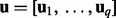

• .

Now we have

(30)

In the following simulation studies (Sections 6.2 and 6.3), we set n = 100, p = 100 and q = 200. To evaluate the performance under different signal-to-noise ratios, we define and as:

(31)

Parameters τ and can be used to control and . An example of synthesized datasets is given in the Supplementary Document.

6.2 Influence of parameter tuning

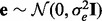
Before we compare LORS with some other methods, we would like to empirically evaluate our parameter tuning procedure. Given a dataset, we need to randomly partition the observed entries into two parts: and . Basically, we train our model based on for different parameters and choose a good parameter configuration such that the trained model has an accurate prediction on . There may be two concerns: (i) Because the random partition may introduce randomness in our modeling process, does this strategy provide a stable parameter selection? (ii) Can this strategy adapt to different noise level? To answer these questions, we do 100 random partitions of a synthetic dataset, and run our method based on each partition separately. The distribution of the selected parameters is shown in Figure 1. First, one can see that the selected parameters do not change a lot during 100 random partitions. The stability of our method should be attributed to the continuity property of the norm (Fan and Li, 2001), that is, a small change of dataset will not cause a big change of the optimization solution. Second, when the signal becomes weaker, i.e. (the left panel of Fig. 1) reduces to (the right panel of Fig. 1), a larger ρ will be selected to prevent the noise from entering the model. This shows that our parameter tuning strategy can adapt to different noise levels. In Section 3.2 of the Supplementary Document, we provide more evidence to show that the random partition in our parameter tuning has little effects on eQTL mapping (i.e. the estimation of matrix ).

Fig. 1.

The distribution of selected parameters (100 random partitions of training and testing data) for synthetic datasets. Left panel: the synthetic dataset is generated with n = 100, p = 100, q = 200, and . For the parameter λ, and are selected in the sequence of λ values in most cases; for parameter ρ, is selected in most cases. Right panel: the synthetic dataset is generated with n = 100, p = 100, q = 200, and . For λ, and are often selected; for ρ, is selected in most cases

6.3 Performance evaluation

We will mainly compare our method LORS with PANAMA. The reasons are: (i) PANAMA can be regarded as an extension of LMM-EH as we discussed above. (ii) Fusi et al. (2012) showed that PANAMA significantly outperforms other related methods, including SVA, PEER and ICE. Here we include the results from standard linear regression as reference, and compare LORS, LORS-Screening and PANAMA with the standard linear regression.

To compare our method with PANAMA under different settings, we vary , and K. For each setting, we report the averaged result from 50 realizations. Figure 2 shows the comparison results for different combinations of , and K (more simulation results can be found in the Supplementary Document). From these simulation results, we can see the following:

• When the number of hidden factors increases, the performance of both LORS and PANAMA degrades slightly.

• When the genetic effects and non-genetic effects are small (compared with noises), e.g. , ), LORS is only comparable with standard linear regression and PANAMA is even worse. This is because the noise plays a dominant role here, it is difficult to account for non-genetic effects under this situation.

• As the genetic effects and non-genetic effects become more apparent, both LORS and PANAMA perform better than standard linear regression. As we mentioned in Section 5.1, LORS and PANAMA share the same model structure, and they differ in how the model structure is inferred. We suspect that PANAMA may be trapped at a local optimum during its model optimization. As a result, LORS may have better performance than PANAMA.

• Regarding to LORS-Screening, it turns out that LORS-Screening is slightly worse than LORS but comparable with PANAMA. Because the computational cost is largely reduced, it is preferred in large data analysis.

Fig. 2.

The ROC curves for performance comparison. (A) The number of hidden factors K = 10. (B) The number of hidden factors K = 30. In each panel, we vary to compare the performance of LORS, PANAMA and standard linear regression

6.4 Estimate of false discovery rate

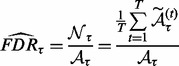
Owing to lack of statistical tests, it is necessary to provide a way to estimate the FDR of our method. Because correlation exists among the rows and columns of , exactly estimating FDR becomes difficult. Here we follow the strategy of (Tibshirani and Wang, 2008; Nowak et al., 2011) to obtain a rough estimator of the true FDR, which may serve as a guideline when applying our method. We use

(32)

as a rough estimator for FDR, where is the number of associations identified at threshold τ under the null distribution, is the number of associations identified at threshold τ in the original dataset. We use permutation to obtain the number of associations identified under the null distribution. Specifically, for a given threshold τ, we do T permutations. At the t-th permutation, we permute the rows of the expression dataset to generate a null dataset, denoted as . Then, we run LORS on the permuted dataset () and obtain the number of associations by applying the threshold τ to the estimated matrix , denoted as . After T permutations, the final estimation of is given by

(33)

We report estimated FDR based on the simulated data as described in Section 6.1 in Figure 9 of the Supplementary Document. The permutation strategy provides a reasonably good estimate for the true FDR. The estimated FDR often overestimates the true FDR (due to the correlation), and thus, it may serve as a conservative guideline.

6.5 Application to eQTL data from yeast

We applied our method to two yeast datasets for eQTL mapping. The first dataset is from Brem et al. (2002) (GEO accession number GSE 1990), which consists of 7084 probes and 2956 genotyped loci in 112 segregates. The second one comes from Smith and Kruglyak (2008), which includes 5493 probes measured in 109 segregates. Analysis of these two datasets provides us an opportunity to demonstrate the benefit of our method because the two expression data share the same genetic effect but different confounding effects.

The significant linkage peaks given by standard linear regression are shown in Figure 3 (A). We can clearly see the confounding effects that lead to spurious associations. We also show the result given by LORS in Figure 3 (B). In total, LORS has detected about 10 000 associations according to non-zero values. Because LORS does not perform statistical significance tests, we are not able to report our result based on statistical significance. In practice, people may be more interested in the top signals that will be followed up for replications. Thus, we only show the top 1000 associations based on the absolute value of . The plots of all associations are also given in the Supplementary Document for completeness. It can be seen that the confounding effects are successfully accounted by LORS, and thus spurious associations are greatly reduced. To quantitatively evaluate the ability of accounting for confounding effects, we compare the reproducibility of the results given by LORS and PANAMA. We examine the reproducibility based on the following two criteria:

• The consistency of detected SNP-gene associations. Let and be the sets of SNP-gene associations detected in the two yeast datasets, respectively. The most T significant associations from the two datasets are denoted as and . The consistency is defined as , where denotes the size of . For LORS, the ranking is based on the absolute value of . For PANAMA, the ranking is based on the q-value.

• The consistency of detected hotspots. For a SNP, we can count the number of associated genes from the detected SNP-gene associations (for LORs, all SNP–Gene pairs with a non-zero B are defined as associations. For PANAMA, SNP–Gene pairs with a q-value <0.001 are defined as associations, we tried different cutoffs from 0.01 to 0.001, the results are similar), i.e. the regulatory degree of the SNP. SNPs with large degrees are often referred to as hotspots. According to SNPs’ regulatory degrees, we sort them in a descending order and denote the sorted SNPs lists as and for the two yeast datasets. Let and be the top T SNPs in the sorted SNP lists, respectively. The consistency of detected hotspots is defined as .

Fig. 3.

(A) A plot of significant linkage peaks given by standard linear regression (P < 0.01 after Bonferroni correction) for expression QTL in the study (Smith and Kruglyak, 2008) by marker location (x-axis) and expression trait location (y-axis). (B) The plot of linkage peaks in the study (Smith and Kruglyak, 2008) given by LORS (Top 1000 associations based on are shown here. The plot of All associations are given in the supplementary document)

For Brem’s dataset (Brem et al., 2002), the estimated sparse matrix given by LORS has about 6000 non-zero entries in total. Among them, there are 4500 entries with abs and 2500 entries with abs , respectively. For Simth’s dataset (Smith and Kruglyak, 2008), the estimated has about 10 000 non-zero entries in total. There are about 4500 entries with abs . (To provide a meaningful guideline of the thresholds, we estimate FDR using 50 permutations. The estimated FDR corresponding to different thresholds are provided in the Supplementary Document. It tells us that FDR 0.01 when threshold 0.01). In Figure 4, we show the consistency of the top 4500 associations. The consistencies of hotspots are shown in Figure 5. It seems to be counter-intuitive that the fraction of consistency of PANAMA increases as the number of detected association increases. In fact, the consistency of PANAMA increases to 0.12 and then drops. We provide the detailed information in the Supplementary Document. From Figures 4 and 5, it can be seen that LORS achieves better consistency than PANAMA.

Fig. 4.

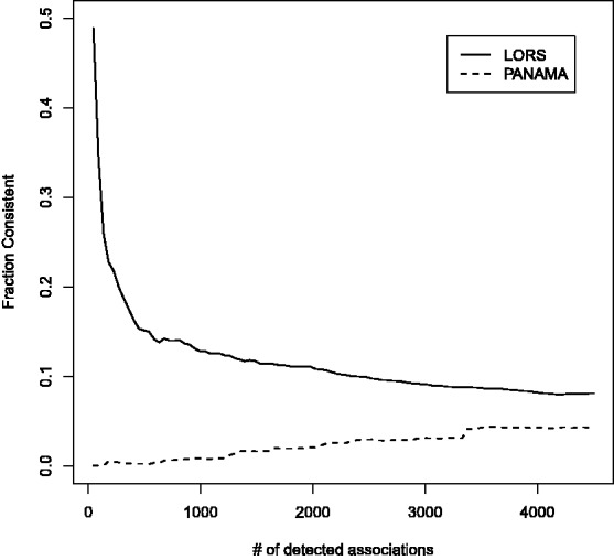
Consistency of detected associations between two independent yeast eQTL datasets

Fig. 5.

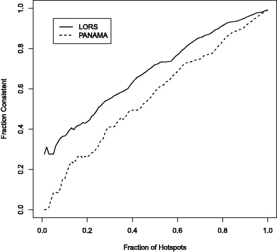
Consistency of detected eQTL hotspots between two independent yeast eQTL datasets

So far we have shown that spurious associations can be reduced by successfully accounting for non-genetic effects. Now we are going to show whether it could help to detect more biologically relevant associations. We take a closer inspection of the top 15 hotspots, as listed in Table 1. In most cases (12/15), associated genes are enriched with at least one GO category, which implies that they are biologically relevant findings. In particular, we detect two novel hotspots (NO. 9 and NO. 13), which can not be detected by standard linear regression (adjusted P ). For these two hotspots, the associated genes are enriched in GO categories. In detail, for hotspot NO. 9, five of the 18 associated genes are functional in response to toxin, they are AAD4, YDL218W, YLL056C, AAD6 and SPS100. The hotspot eQTL is cis-linked to one of them, AAD4, which apparently explains the detected association. Hotspot NO. 13 locates at transcription factor (TF) CAT8. Based on the transcriptional regulation information in yeast from both direct (Chip-chip) or indirect (Microarrays—wild type versus TF mutant) evidence (Teixeira et al., 2006), 9 (they are ADY2, PUT4, GAP1, ATO3, ALP1, YDR222w, CWP1, ADH2 and LPX1) of the 15 associated genes can be potentially regulated by CAT8 (adjusted P , the details of the p-value calculation is given in the Supplementary Document). Interestingly, five genes (i.e. ADY2, PUT4, GAP1, ATO3, ALP1) are functional in organic acid transport and CAT8 is known to regulate acid transport pathway (Young et al., 2003). Identification of this hotspot provides a positive example and indicates that, when non-genetic effect has been successfully accounted for, we may be able to detect more biologically relevant trans eQTL.

Table 1.

Summary of the detected hotspots

Hotspot index	Sizea	Locib	GO categoryc	Hitsd	t-test (all)e	t-test (hits)f
NO. 1	32	Chr XII:1056103	Telomere maintenance via recombination	5	20	5
NO. 2	27	Chr IV:1525327	Telomere maintenance via recombination	4	5	3
NO. 3	26	Chr XII:662627	Sterol metabolic process	7	25	7
NO. 4	24	Chr I:52859	Fatty acid metabolic process	10	12	6
NO. 5	24	Chr XV:202370	Response to abiotic stimulus	10	11	6
NO. 6	23	Chr III:201166	Response to pheromone	7	16	6
NO. 7	21	Chr VII:402833	Protein folding	8	4	3
NO. 8	19	Chr I:7298	Fatty acid beta-oxidation	5	13	4
NO. 9	18	Chr IV:33214	Response to toxin	5	0	0
NO. 10	16	Chr II:562415	Cytokinesis	8	15	8
NO. 11	16	Chr X:698149	—	—	3	—
NO. 12	16	Chr XV:132423	—	—	13	—
NO. 13	15	Chr XIII:843356	Organic acid transport	5	0	0
NO. 14	15	Chr V:395442	—	—	3	—
NO. 15	15	Chr XVI:486637	Sexual reproduction	6	8	4

^aNumber of genes associated with the hotspot. ^bThe chromosome position of hotspot. ^cThe most significant GO category enriched in the associated gene set. The enrichment test was performed using DAVID (Huang da and Lempicki, 2008). The gene function is defined by GO Fat category. DAVID outputs the Benjamini–Hochberg adjusted P-value. Adjusted P-values are indicated by , where ^dNumber of associated genes that are functional in the enriched GO category. ^eNumber of associated genes that can also be identified using t-test. ^fNumber of associated genes that are functional in the enriched GO category and can also be identified using t-test. Two novel hotspots (NO. 9 and NO. 13) which cannot be detected by standard linear regression are in bold.

7 CONCLUSIONS

In this article, we have introduced a method named ‘LORS’ to account for non-genetic effects in eQTL mapping. LORS provided a unified framework in which all SNPs and all gene probes can be jointly analyzed. The formulation of LORS is a convex optimization problem and thus its global optimum can be achieved. We also developed an efficient algorithm to solve this problem and guaranteed its convergence. We demonstrated its performance using synthetic datasets and real datasets.

A limitation of LORS is that we do not provide a rigorous statistical significance test of the estimated coefficient matrix . Here we simply rank associations based on the estimated sparse matrix abs() and estimate FDR.

Funding: This work was supported in part by NSF (DMS 1106738), NIH (R01 GM59507) and NSFC (10901042, 10971075 and 91130032).

Conflict of Interest: none declared.

REFERENCES

- Alter O, et al. Singular value decomposition for genome-wide expression data processing and modeling. Proc. Natl Acad. Sci. USA. 2000;97:10101–10106. doi: 10.1073/pnas.97.18.10101. [DOI] [PMC free article] [PubMed] [Google Scholar]
- Brem RB, et al. Genetic dissection of transcriptional regulation in budding yeast. Science. 2002;296:752–755. doi: 10.1126/science.1069516. [DOI] [PubMed] [Google Scholar]
- Cheung V, Spielman R. Genetics of human gene expression: mapping dna variants that influence gene expression. Nat. Rev. Genet. 2009;10:595–604. doi: 10.1038/nrg2630. [DOI] [PMC free article] [PubMed] [Google Scholar]
- Cookson W, et al. Mapping complex disease traits with global gene expression. Nat. Rev. Genet. 2009;10:184–194. doi: 10.1038/nrg2537. [DOI] [PMC free article] [PubMed] [Google Scholar]
- Huang da W, et al. Systematic and integrative analysis of large gene lists using david bioinformatics resources. Nat. Protoc. 2008;4:44–57. doi: 10.1038/nprot.2008.211. [DOI] [PubMed] [Google Scholar]
- Fan J, Li R. Variable selection via nonconcave penalized likelihood and its oracle properties. J. Am. Stat. Assoc. 2001;96:1348–1360. [Google Scholar]
- Fan J, Lv J. Sure independence screening for ultrahigh dimensional feature space. J. R. Stat. Soc. Series B Stat. Methodol. 2008;70:849–911. doi: 10.1111/j.1467-9868.2008.00674.x. [DOI] [PMC free article] [PubMed] [Google Scholar]
- Friedman J, et al. Pathwise coordinate optimization. Ann. Appl. Stat. 2007;1:302–332. [Google Scholar]
- Friedman J, et al. Regularization paths for generalized linear models via coordinate descent. J. Stat. Softw. 2010;33:1–22. [PMC free article] [PubMed] [Google Scholar]
- Fusi N, et al. Joint modelling of confounding factors and prominent genetic regulators provides increased accuracy in genetical genomics studies. PLoS Comput. Biol. 2012;8:e1002330. doi: 10.1371/journal.pcbi.1002330. [DOI] [PMC free article] [PubMed] [Google Scholar]
- Gagnon-Bartsch J, Speed T. Using control genes to correct for unwanted variation in microarray data. Biostatistics. 2012;13:539–552. doi: 10.1093/biostatistics/kxr034. [DOI] [PMC free article] [PubMed] [Google Scholar]
- Gibson G. The environmental contribution to gene expression profiles. Nat. Rev. Genet. 2008;9:575–581. doi: 10.1038/nrg2383. [DOI] [PubMed] [Google Scholar]
- Kang H, et al. Accurate discovery of expression quantitative trait loci under confounding from spurious and genuine regulatory hotspots. Genetics. 2008;180:1909–1925. doi: 10.1534/genetics.108.094201. [DOI] [PMC free article] [PubMed] [Google Scholar]
- Kang H, et al. Variance component model to account for sample structure in genome-wide association studies. Nat. Genet. 2010;42:348–354. doi: 10.1038/ng.548. [DOI] [PMC free article] [PubMed] [Google Scholar]
- Leek J, Storey J. Capturing heterogeneity in gene expression studies by surrogate variable analysis. PLoS Genet. 2007;3:e161. doi: 10.1371/journal.pgen.0030161. [DOI] [PMC free article] [PubMed] [Google Scholar]
- Leek J, et al. Tackling the widespread and critical impact of batch effects in high-throughput data. Nat. Rev. Genet. 2010;11:733–739. doi: 10.1038/nrg2825. [DOI] [PMC free article] [PubMed] [Google Scholar]
- Li C, Rabinovic A. Adjusting batch effects in microarray expression data using empirical Bayes methods. Biostatistics. 2007;8:118–127. doi: 10.1093/biostatistics/kxj037. [DOI] [PubMed] [Google Scholar]
- Li L, et al. eQTL. Methods Mol. Biol. 2012;871:265–279. doi: 10.1007/978-1-61779-785-9_14. [DOI] [PubMed] [Google Scholar]
- Lippert C, et al. Fast linear mixed models for genome-wide association studies. Nat. Methods. 2011;8:833–835. doi: 10.1038/nmeth.1681. [DOI] [PubMed] [Google Scholar]
- Listgarten J, et al. Correction for hidden confounders in the genetic analysis of gene expression. Proc. Natl Acad. Sci. USA. 2010;107:16465–16470. doi: 10.1073/pnas.1002425107. [DOI] [PMC free article] [PubMed] [Google Scholar]
- Mazumder R, et al. Spectral regularization algorithms for learning large incomplete matrices. J. Mach. Learn. Res. 2010;11:2287–2322. [PMC free article] [PubMed] [Google Scholar]
- Nica A, Dermitzakis E. Using gene expression to investigate the genetic basis of complex disorders. Hum. Mol. Genet. 2008;17(R2):R129–R134. doi: 10.1093/hmg/ddn285. [DOI] [PMC free article] [PubMed] [Google Scholar]
- Nielsen T, et al. Molecular characterisation of soft tissue tumours: a gene expression study. Lancet. 2002;359:1301–1307. doi: 10.1016/S0140-6736(02)08270-3. [DOI] [PubMed] [Google Scholar]
- Nowak G, et al. A fused lasso latent feature model for analyzing multi-sample aCGH data. Biostatistics. 2011;12:776–791. doi: 10.1093/biostatistics/kxr012. [DOI] [PMC free article] [PubMed] [Google Scholar]
- Pastinen T, et al. Influence of human genome polymorphism on gene expression. Hum. Mol. Genet. 2006;15(Suppl. 1):R9. doi: 10.1093/hmg/ddl044. [DOI] [PubMed] [Google Scholar]
- Rasmussen C, Williams C. Gaussian Processes in Machine Learning. Cambridge, MA, USA: The MIT Press; 2006. [Google Scholar]
- Recht B, et al. Guaranteed minimum-rank solutions of linear matrix equations via nuclear norm minimization. SIAM Rev. 2010;52:471–501. [Google Scholar]
- Shi L, et al. The microarray quality control (MAQC) project shows inter-and intraplatform reproducibility of gene expression measurements. Nat. Biotechnol. 2006;24:1151–1161. doi: 10.1038/nbt1239. [DOI] [PMC free article] [PubMed] [Google Scholar]
- Smith EN, Kruglyak L. Gene-environment interaction in yeast gene expression. PLoS Biol. 2008;6:e83. doi: 10.1371/journal.pbio.0060083. [DOI] [PMC free article] [PubMed] [Google Scholar]
- Stegle O, et al. A Bayesian framework to account for complex non-genetic factors in gene expression levels greatly increases power in eQTL studies. PLoS Comput. Biol. 2010;6:e1000770. doi: 10.1371/journal.pcbi.1000770. [DOI] [PMC free article] [PubMed] [Google Scholar]
- Teixeira M, et al. The yeastract database: a tool for the analysis of transcription regulatory associations in Saccharomyces cerevisiae. Nucleic Acids Res. 2006;34(Suppl. 1):D446–D451. doi: 10.1093/nar/gkj013. [DOI] [PMC free article] [PubMed] [Google Scholar]
- Tibshirani R. Regression shrinkage and selection via the lasso. J. R. Stat. Soc. Series B. 1996;58:267–288. [Google Scholar]
- Tibshirani R, Wang P. Spatial smoothing and hot spot detection for CGH data using the fused lasso. Biostatistics. 2008;9:18–29. doi: 10.1093/biostatistics/kxm013. [DOI] [PubMed] [Google Scholar]
- Young E, et al. Multiple pathways are co-regulated by the protein kinase Snf1 and the TFs Adr1 and Cat8. J. Biol. Chem. 2003;278:26146–26158. doi: 10.1074/jbc.M301981200. [DOI] [PubMed] [Google Scholar]
Associated Data
This section collects any data citations, data availability statements, or supplementary materials included in this article.