EBSeq: an empirical Bayes hierarchical model for inference in RNA-seq experiments

Abstract

Motivation: Messenger RNA expression is important in normal development and differentiation, as well as in manifestation of disease. RNA-seq experiments allow for the identification of differentially expressed (DE) genes and their corresponding isoforms on a genome-wide scale. However, statistical methods are required to ensure that accurate identifications are made. A number of methods exist for identifying DE genes, but far fewer are available for identifying DE isoforms. When isoform DE is of interest, investigators often apply gene-level (count-based) methods directly to estimates of isoform counts. Doing so is not recommended. In short, estimating isoform expression is relatively straightforward for some groups of isoforms, but more challenging for others. This results in estimation uncertainty that varies across isoform groups. Count-based methods were not designed to accommodate this varying uncertainty, and consequently, application of them for isoform inference results in reduced power for some classes of isoforms and increased false discoveries for others.

Results: Taking advantage of the merits of empirical Bayesian methods, we have developed EBSeq for identifying DE isoforms in an RNA-seq experiment comparing two or more biological conditions. Results demonstrate substantially improved power and performance of EBSeq for identifying DE isoforms. EBSeq also proves to be a robust approach for identifying DE genes.

Availability and implementation: An R package containing examples and sample datasets is available at http://www.biostat.wisc.edu/∼kendzior/EBSEQ/.

Contact: kendzior@biostat.wisc.edu

Supplementary information: Supplementary data are available at Bioinformatics online.

1 INTRODUCTION

Appropriate expression of a gene’s isoforms via alternative splicing is fundamental to normal development and maintenance in eukaryotes, and aberrations in alternative splicing are common in disease (Smith et al., 1989; Stamm et al., 2005; Wang et al., 2008). Consequently, there is much interest in identifying isoforms with expression that varies on average across biological conditions. High-throughput cDNA sequencing (RNA-seq) experiments provide the potential to identify such differentially expressed (DE) isoforms on a genome-wide scale, but statistical methods are required to ensure that accurate identifications are made.

The statistical methods available for identifying differences in isoforms in an RNA-seq experiment [e.g. MISO (Katz et al., 2010), FDM (Singh et al., 2011), Chi-Square test in Howard and Heber (2010)] have focused on changes in the proportion of gene-specific reads assigned to an isoform, so-called differential transcription (DT) or differential splicing (DS). These methods do not consider changes in overall expression levels and are therefore not appropriate for identifying DE isoforms. For example, consider a gene with two isoforms: the first with average counts 500 and 1500 in conditions 1 and 2, respectively, the second with average counts 1000 and 3000 in the two conditions, respectively. These isoforms would not be DT or DS, given that the proportion of total reads assigned to each isoform is unchanged across conditions (1/3 for isoform 1 and 2/3 for isoform 2), but the isoforms would likely be called DE, given there is a 3-fold increase in expression in the second condition. When isoform-level DE calls are required, count-based methods developed for identifying DE genes are often applied directly to estimates of isoform expression (Sandmann et al., 2011). Doing so is not optimal.

The main problem is that count-based methods expect counts, or more specifically, an integer summary of reads mapping to a gene’s constituent exons, and they were not designed to accommodate the differential uncertainty induced by isoform expression estimation. In short, prior to isoform DE inference, each isoform’s expression must be estimated from aligned reads. For genes with a single isoform, this problem is rather straightforward in that all reads mapping to that gene are used to estimate that isoforms’ expression. For genes with multiple isoforms, isoform expression estimation is more difficult, as reads mapping to exons common to multiple isoforms must be allocated in a way consistent with each isoform’s expression level, which is the very quantity being estimated. There are a number of methods available for estimating isoform expression [RSEM (Li and Dewey, 2011), RSeq (Jiang and Wing, 2009), IsoEM (Nicolae et al., 2010), Cufflinks (Trapnell et al., 2012) and IQSeq (Du et al., 2012)]. Whatever method used, due to the increased difficulty inherent in estimating isoform expression for isoforms with common constitutive exons, there are varying levels of uncertainty in isoform expression estimates (see Fig. 1). Most approaches for identifying DE in an RNA-seq experiment focus on genes [DESeq (Anders and Huber, 2010), edgeR (Robinson and Smyth, 2007), baySeq (Hardcastle and Kelly, 2010), BBSeq (Zhou et al., 2011)], and do not accommodate this differential uncertainty. Consequently, they are not appropriate for identifying DE isoforms. Another recently developed approach [DEXSeq (Anders et al., 2012)] may be used for identifying DE exons, but does not provide information on which associated isoforms are DE.

Fig. 1.

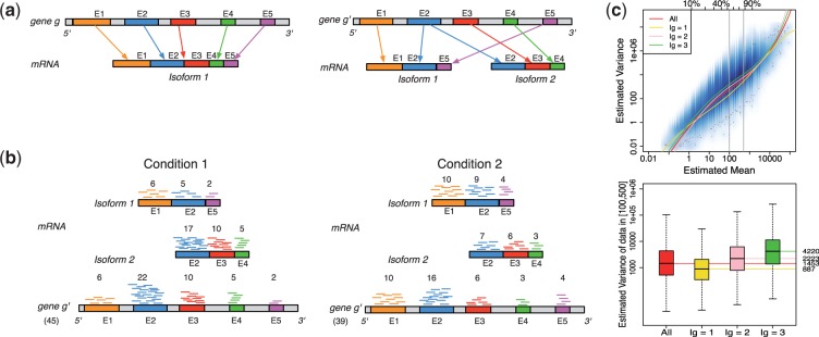
Panel (a) shows two hypothetical genes g and . Gene g has one isoform, denoted by ; gene has two (). The problem of estimating expression for isoforms of is complicated by the fact that reads mapping to exon 2 must be unambiguously assigned to each isoform. This results in increased uncertainty, on average, in expression estimates for isoforms sharing a parent. Panel (b) shows hypothetical expression of the isoforms from gene in each of two conditions (assuming differences in library size have been accommodated). If one focuses on the longest isoform (isoform 1) and uses all reads mapping to its constituent isoforms to estimate its expression, the isoform is called equivalently expressed, as there are 30 (6 + 22 + 2) reads mapped in condition 1 and 30 (10 + 16 + 4) mapped in condition 2. However, if the expression of other isoforms is considered, it becomes clear that isoform 1 contains almost twice as many reads in condition 2 as in condition 1 (23 versus 13, respectively). Panel (c) demonstrates how estimation uncertainty changes as isoform complexity increases. We quantified isoform complexity here by I_g where the group represents isoforms from genes with k isoforms (here isoforms from genes with more than three isoforms are included in the group; alternative definitions of complexity are discussed in the text). Shown top right are splines fit to the empirical variance as a function of the mean for all isoforms as well as isoforms within groups defined by I_g for the two-group human embryonic stem cell RNA-seq experiment described in Section 2; bottom right considers isoforms with average expression (expected count) in [100, 500]. The range was chosen as it approximates the 50th and 80th percentiles of expression across all isoforms. Shown are box plots of the variances of these isoforms collectively, and within I_g group. Median variance within each group is shown right

When isoform DE is of interest, some count-based methods (e.g. edgeR) suggest choosing a single isoform [such as the isoform with the most counts within a gene or the longest isoform (Sandmann et al., 2011)] and estimating expression using reads mapping to the isoforms’ constituent exons. In either case, information on other isoforms is lost, and reads mapping to multiple genes are ignored. A more serious consideration is that erroneous conclusions may be made due to differences in other isoforms (see Fig. 1b for an example). Other methods such as easyRNASeq suggest that one assign all reads mapping to overlapping exons to each isoform separately (i.e. count reads mapping to exon 2 in Fig. 1b twice, once for each isoform), and then proceed with a count-based approach. As with the prior suggestion, this can lead to erroneous conclusions. Specifically, an isoform may appear to be equally expressed (EE, say isoform 1 in Fig. 1b), even if it is not.

A potentially more robust way to proceed is to estimate each isoform’s mRNA counts using a method designed specifically to do so (Jiang and Wing, 2009; Li and Dewey, 2011; Nicolae et al., 2010; Trapnell et al., 2012) and then apply a count-based approach directly to expected counts after rounding the expected counts to the nearest integer. This, too, is not advised. Count-based methods require gene-level counts and consequently do not account for uncertainty inherent in estimated counts. Furthermore, given that uncertainty varies systematically for different groups of isoforms, applications of count-based approaches for isoform level inference result in reduced power for some classes of isoforms and increased false discoveries for others. In short, the test statistics used by most methods for DE gene identification calibrate a difference in expression levels between conditions by a variance, which is commonly estimated using the mean–variance relationship observed in data. Figure 1c shows that this relationship varies dramatically for different groups of isoforms, where groups are defined by the number of constituent isoforms of the parent gene (other definitions are possible as discussed below). Specifically, an isoform of gene g is assigned to the group, for example, where or 3, if the total number of isoforms from gene g is k (the group contains all isoforms from genes having 3 or more isoforms).

As shown in Figure 1c, there is decreased variability in the group, but increased variability in the others, due to the relative increase in uncertainty inherent in estimating isoform expression when multiple isoforms of a given gene are present. This observation is not specific to the dataset and/or the method used for isoform expression estimation; it is also not specific to the particular method used for quantifying isoform complexity (see Supplementary Figs S1–S4 for additional examples). If isoforms are analysed collectively, there is reduced power for identifying isoforms in the group (since the true variances in that group are lower, on average, than those derived from the full collection of isoforms) and increased false discoveries in the and groups (since the true variances are higher, on average, than those derived from the full collection). These effects are demonstrated in a simulation study in Section 4 of the Supplementary Material.

Cuffdiff2 (Trapnell et al., 2013) and BitSeq (Glaus et al., 2012) account for differential uncertainty in isoform expression estimates and thus appropriately accommodate DE inference at the isoform level. However, Cuffdiff2 often finds fewer genes than comparable approaches, and the simulations here suggest this is a result of lack of power, as opposed to an increased false discovery rate (FDR) of other methods. BitSeq is a good alternative when ranking isoforms is of interest, but it does not provide a way to control a list of identifications at a desired level of FDR. Finally, both approaches couple expression estimation with DE inference, and are not applicable to expression estimates obtained separately (e.g. via RSEM or one of the other methods mentioned above). As other expression-estimation methods have demonstrated higher precision and continue to be improved, methods for DE inference that accept expression estimates directly are desirable.

Taking advantage of the merits of empirical Bayesian (EB) methods, we developed an approach called EBSeq for inference in an RNA-seq experiment. Although its main advantage over other approaches is in its ability to identify DE isoforms, results from simulations and case studies demonstrate good performance for identification of DE genes as well.

2 METHODS

2.1 EBSeq: an empirical Bayes model for identifying DE genes and isoforms

EBSeq requires gene counts or estimates of isoform expression, but it is not specific to any particular estimation method (e.g. RSEM, Rseq, Cufflinks or another method may be used). The general model is developed for isoform analysis. The gene-level model is a special case discussed at the end of this section. The model assumes the expected count for isoform i in gene g and sample s is distributed as Negative Binomial, , where , and ; N_g denotes the number of isoforms of gene g. Specifically, we assume that within condition C, 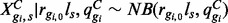, where l_s represents the library size in sample s and may be defined as the total number of reads or obtained by TMM (Robinson and Oshlack, 2010), Median Normalization (Anders and Huber, 2010) or Upper Quartile Normalization (Bullard et al., 2010). Since the total number of reads may be adversely affected by outliers from PCR or other artifacts, the latter three methods are recommended. The EBSeq code defaults to Median Normalization, but Quantile Normalization is also available. Within this framework, the mean and variance are given by: 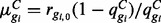and .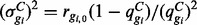

A prior distribution describes fluctuations in technical and biological variation: 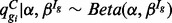. The hyper-parameter α is shared across isoforms while β depends on I_g, accommodating the systematic differences in variability among the I_g groups. I_g quantifies a measure of isoform complexity and may be defined by the user as the number of isoforms from a gene, as described in the previous section, or from an isoform’s mappability score or credibility interval as provided by some isoform expression-estimation approaches.

When RNA-seq reads in two biological conditions are available, identifying DE isoforms corresponds to identifying those isoforms for which . Since is common across conditions, this is analogous to identifying those isoforms for which . Letting p denote the prior probability of DE, counts are modelled by the mixture distribution where represents g_i’s read counts across the two conditions; f₀ and f₁ are the predictive distributions under EE and DE, respectively:

(1)

and

(2)

Estimates of the isoform-specific means and variances are obtained via method-of-moments, and the four global hyper-parameters (α, , and ) are obtained via the expectation-maximization (EM) algorithm (Dempster et al., 1977) (see Section 6 of the Supplementary Material for further details). With parameter estimates in hand, the posterior probability of DE (or EE) is obtained via Bayes’ rule. A mixture model with additional components may be used when data from more than two conditions are available (an example is provided in Section 6 of the Supplementary Material). Unless otherwise noted, all calculations were carried out in R (R Development Core Team, 2009); package and annotation versions are given in Section 1 of the Supplementary Material.

2.2 Simulated data

We followed the simulation set-up of Robinson and Smyth (2007) by defining counts as Negative Binomial with isoform-specific mean in sample s and condition C given by and variance . The library size factors for both the isoform and gene-level simulations were randomly simulated from Uniform (0.8, 1.3). One hundred simulated datasets were generated for each scenario considered.

Sim I: Isoform expression for each of 30 802 isoforms, four lanes in each of two conditions, is generated by sampling unknown parameters from the case study comparing embryonic stem cells (ESCs) with induced pluripotent stem cells (iPSCs). The number of isoforms and sample sizes are taken to match those in the case study. The percentages of DE isoforms were set at 2, 4 and 5% in the and 3 groups, also to match the case study data. Parameters for isoforms belonging to the same gene are sampled together to preserve dependence within isoforms common to a single gene. For DE isoforms, where is sampled from the 95–97% quantile of fold changes in sample means across conditions; for EE isoforms .

Sim II: Isoform expression for each of 30 802 isoforms is generated by sampling from case study data; is fixed for all g_i. Six sets of simulations are considered to investigate the effects of systematic changes in variability, one set for each ϕ in (, , , , , ); DE and EE are as in Sim I. This set-up is similar to that considered in Robinson and Smyth (2007). There, too, is sampled and ϕ is fixed, but here we simulate isoforms (not genes) and we consider more (and slightly different values) of ϕ. An evaluation of the exact simulation set-up considered in Robinson and Smyth (2007) is given in Supplementary Figure S8.

Sim III: Gene expression for each of 20 000 genes is generated by sampling unknown parameters from case study data. Two per cent DE genes are simulated to match the case study data.

The Supplementary Material provides details on additional simulations (see Supplementary Material Section 4) and demonstrates that characteristics observed in the case study data are reproduced in the simulated datasets considered here (see Supplementary Fig. S5). Supplementary Figure S8 also shows results from the simulations considered in the articles introducing edgeR and baySeq.

2.3 Experimental data

2.3.1 MicroArray Quality Control data

The raw read files (fasta format) were downloaded from SRA SRX016359 and SRX016367. As part of the MicroArray Quality Control (MAQC) project, RNA was extracted from one sample of human brain tissue (HBR) and one sample of mixtures of tissues (UHR); seven replicates from each sample are considered here. To obtain gene counts using HTSeq, reads were aligned to the human RefSeq Hg18 transcripts using Bowtie (Langmead et al., 2009) and TopHat (Trapnell et al., 2009), allowing for no multiple matches (HTSeq requires that multi-reads are discarded) and two mismatches. HTSeq was applied to obtain gene counts for 18 780 genes, in which 16 518 were expressed (with median expression greater than 0). To obtain estimates of expression via Cufflinks (Trapnell et al., 2010), Bowtie and Tophat were applied allowing for up to 20 multiple matches and two mismatches. Expression was then estimated using Cufflinks (Trapnell et al., 2010) for 18 780 genes and 30 802 isoforms, in which 17 152 genes and 26 210 isoforms were expressed.

2.3.2 Thomson Lab data; ES versus iPS cell lines

We analysed RNA-seq data from the James Thomson Lab at the Morgridge Institute for Research at UW-Madison. Details on the samples are given in Phanstiel et al. (2011); the particular samples considered here as well as alignment and expression estimation vary from that reported in Phanstiel et al. (2011) as follows. We evaluate RNA-seq reads from embryonic stem (ES) cell lines H1, H7, H9 and H14 and induced pluripotent stem (iPS) cell lines DF4.7, DF6.9, DF19.7 and DF19.11. We filter 42-base pair reads to remove adapters in each lane. To obtain gene counts via HTSeq, reads were aligned to the human RefSeq Hg18 transcripts using Bowtie and TopHat, allowing for no multiple matches and two mismatches. HTSeq was then applied to obtain gene counts for 18 780 genes, in which 15 671 were expressed. To obtain estimates of gene and isoform expression via Cufflinks, Bowtie and Tophat were applied, allowing for up to 20 multiple matches and two mismatches. Expression was then estimated using Cufflinks.

Two other datasets (Gould Lab and Smith Lab) are shown in Figure 2c; details on these datasets may be found in Section 2 of the Supplementary Material.

Fig. 2.

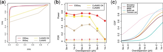
Panel (a) shows ROC curves (TPR versus FPR). The curves are obtained from averaging over 100 Sim I simulations. Cuffdiff2 deems some isoforms unacceptable prior to analysis; isoforms deemed acceptable by Cuffdiff2 are denoted ‘OK’; and results are reported here for both (see Section 2 for more details). Panel (b) shows the operating characteristics of EBSeq and Cuffdiff2 as a function of ϕ, described in Sim II. The solid and dashed lines indicate power (TPR) and FDR, respectively, at 5% target FDR. Note that BitSeq provides a PPLR for rank ordering isoforms, but does not detail how to use the PPLR scores to control FDR for two-sided test. Consequently, BitSeq is evaluated when ranking isoforms in Panel (a), but not when FDR-controlled lists are considered in Panel (b). Panel (c) shows the CDF of ϕ in four empirical datasets, detailed in Section 2 and the Supplementary Material, as well as the CDF averaged across 100 Sim I simulations

2.4 Identification of DE genes and isoforms

EBSeq is compared with baySeq (1.1.0), BitSeq (1.2.1), Cuffdiff2 (2.0.1), DESeq (1.8.2) and edgeR (2.6.3). Further information on package defaults, annotation versions and other software is given in Section 1 of the Supplementary Material. To quantify evidence in favour of DE, EBSeq and baySeq provide posterior probabilities whereas DESeq, edgeR and Cuffdiff2 provide P-values, which are adjusted for multiplicities using Benjamini–Hochberg (DESeq, edgeR) or by converting to q-values (Cuffdiff2). To construct a list of DE genes/isoforms with target two-sided FDR a, we considered those genes/isoforms for which the posterior probability of DE was ≥ (baySeq and EBseq) or those genes/isoforms for which adjusted P-values were ≤a (DESeq, edgeR, Cuffdiff2). BitSeq provides the posterior probability of a positive log-ratio (PPLR) for rank ordering isoforms, but does not detail how to use the PPLR to control FDR for two-sided test. Consequently, BitSeq is evaluated when ranking isoforms, but not when FDR controlled lists are considered.

Non-expressed genes and isoforms are filtered out prior to applying baySeq, DESeq, edgeR and EBSeq. The non-expressed genes and isoforms are defined as the ones with zero median expression across all the samples. Cuffdiff2 also removes genes or isoforms with low expression, but has additional criteria that concern whether an isoform contains enough reads in each locus and whether one or more replicates produce a value for the transcript outside of the confidence interval generated when pooling replicates together. Acceptable isoforms are called ‘OK’ in Cuffdiff2.

2.5 Identification of outliers

To identify putative outliers in the case studies, for each gene we evaluated Dixon’s Q-statistic (Dixon, 1950) as well as the fold change ratio (FCRatio). A Dixon’s Q-statistic for a collection of values is defined as the gap over range, where gap is the absolute difference between the potential outlier in question and the number closest to it; the range is the max minus min. For each gene in each condition, we calculated Dixon’s Q-statistics for the smallest and the largest value. The sample with the largest Dixon’s Q-statistic was defined as the potential outlier for that gene; and the largest Dixon’s Q-statistic (over the two conditions) was taken as the Dixon’s Q-statistic for the gene. The FCRatio is the ratio of the fold change without the outlier over the fold change with the outlier. A gene containing an outlier will have a Dixon’s Q-statistic near 1 and FCRatio far from 1.

3 RESULTS

Simulation studies were conducted to investigate the operating characteristics of EBSeq and to assess how EBSeq compares with competing approaches. As detailed in Section 2, each simulated dataset derives counts from a Negative Binomial model. The Negative Binomial assumption is common to each method considered here (Anders and Huber, 2010; Hardcastle and Kelly, 2010; Robinson and Smyth, 2007; Trapnell et al., 2012), and should therefore not provide advantage, or lack thereof, to any one method in particular. Furthermore, the form of the variance is not one we assumed in EBSeq; rather, it was prescribed in the simulation set-up of Robinson and Smyth (2007). Three sets of simulations are considered here. Additional simulations are evaluated in Section 4 of the Supplementary Material.

For evaluation of isoform-level inference, EBSeq is compared with Cuffdiff2 and BitSeq. It is important to note that Cuffdiff2 and BitSeq are not stand-alone packages that accept counts directly. Rather, Cuffdiff2 requires as input aligned reads that are subsequently processed through Cufflinks to estimate counts; BitSeq is similar, requiring that reads are processed through BitSeq stage 1. This is important, as in the isoform simulation studies (Sims I and II), simulated counts were transformed back to reads as was done in RSEM (Li and Dewey, 2011); the reads were then processed via Cufflinks (or BitSeq stage 1) prior to analysis. The transformation is not possible with simulated gene counts, as multiple read count configurations can give rise to the same overall gene count, and as a result, Cuffdiff2 is not evaluated in the gene simulations; it is evaluated at the gene-level on both MAQC project and case study data. BitSeq is not evaluated in any gene-level analysis, as the PPLR provided for each isoform is derived from isoform-specific Markov Chain Monte Carlo (MCMC) samples, and no information is provided on combining the chains to derive a gene-level PPLR.

3.1 Simulation-based evaluation of EBSeq, Cuffdiff2 and BitSeq for identifying DE isoforms

Table 1 shows the power and FDR for EBSeq and Cuffdiff2 averaged across 100 Sim I simulations for a target FDR of 5%. Cuffdiff2 deems some isoforms unacceptable prior to analysis. Acceptable isoforms are called ‘OK’ in Cuffdiff2, and so results are reported for all genes as well as those deemed ‘OK’ by Cuffdiff2. Because BitSeq provides PPLR for rank ordering isoforms, but does not specify how to use PPLR to construct a list of DE isoforms with a target FDR, it is not shown in Table 1. BitSeq is evaluated in the ROC curves shown in Figure 2.

Table 1.

Isoform simulation results

Methods	Power (%)	FDR (%)
Cuffdiff2	33.6	0.2
Cuffdiff2(OK)	44.4	0.2
EBSeq	72.2	8.2

The empirical power and FDR for EBSeq and Cuffdiff2 averaged across 100 Sim I simulations where target FDR was set at 5%. Cuffdiff2 deems some isoforms unacceptable prior to analysis. Operating characteristics are reported overall, as well as within those deemed acceptable (‘OK’) by Cuffdiff2. Standard errors on average power (FDR) were <2% (0.2%) and are not shown.

As shown in Table 1, Cuffdiff2 has well controlled FDR, but reduced power compared with EBSeq (∼44% versus ∼72%); the FDR of EBSeq is slightly elevated (∼8%). Panel (a) of Figure 2 shows qualitatively similar results for lists of varying size, not determined by targeting a specific FDR. In particular, the ROC curves [empirical true positive rate (TPR) versus empirical false positive rate (FPR) for lists of increasing size] show that the TPR is higher than Cuffdiff2 for lists provided by EBSeq for all FPRs considered. BitSeq also provided higher TPR than Cuffdiff2 across all FPRs, and showed comparable performance with EBSeq.

A closer look into the DE calls from the Sim I simulations reveals that operating characteristics are sensitive to ϕ, which determines within-isoform variability. To demonstrate the effects, panel (b) of Figure 2 shows power and FDR for six other sets of simulations where ϕ is fixed at a specific value (detailed in Sim II). The solid lines show that the power of both methods decreases as variability (ϕ) increases, with a greater loss in power for Cuffdiff2; the dashed lines show that FDR increases slightly but remains well-controlled for both methods. Panel (c) shows the cumulative distribution functions (CDFs) of ϕ in four empirical datasets as well as the average CDF from 100 Sim I simulations to demonstrate that the values of ϕ considered in panel (b) are typical of those observed in data. Panel (c) also demonstrates systematic differences between the three datasets with biological replicates and the MAQC data. Given that the MAQC data is made up of technical replicates, it is not surprising to observe relatively smaller values of ϕ compared with datasets having biological reps. However, since the operating characteristics of DE identification methods vary with ϕ [as shown in panel (b)], an evaluation of methods based on MAQC data alone is cautioned. Below we evaluate methods using MAQC as well as simulated data.

3.2 Evaluation of EBSeq, Cuffdiff2, DESeq, edgeR and baySeq for identifying DE genes using MAQC and simulated data

To evaluate EBSeq as well as other methods for gene-level inference, we use data from the MAQC Project (Consortium, 2006) as well as simulated datasets. The RNA-seq data from the MAQC Project has been widely used to evaluate RNA-seq quantification and normalization methods (Bullard et al., 2010; Li and Dewey, 2011). In particular, Taq-Man qRT-PCR measurements for 1000 genes are available; the 716 of these having consistent annotations in the RefSeq Hg18 reference are often used as a gold-standard for evaluation (for more details, see Li and Dewey, 2011).

To evaluate baySeq, DESeq and edgeR, counts were obtained via HTSeq; expression was estimated via Cufflinks to evaluate Cuffdiff2. Since EBSeq can accept counts or estimated counts as input, it is evaluated on both HTSeq-derived counts as well as Cufflinks-processed data. Of the 716 gold-standard genes, EBSeq and Cuffdiff2 identify 530 and 490 DE genes, respectively, at a target FDR of 5%. Although the majority of identifications are common to both approaches, some insight may be gained by considering those genes identified exclusively by each approach (57 are found by EBSeq but not Cuffdiff2 and 17 are identified by Cuffdiff2 but not EBSeq). The top panel of Figure 3 shows differences in these genes. In particular, the genes identified exclusively by EBSeq reproduce in the RT-PCR measurements [panel (a)], and they have larger fold changes [panel (b)], suggesting that most of the additional genes found by EBSeq are in fact true discoveries.

Fig. 3.

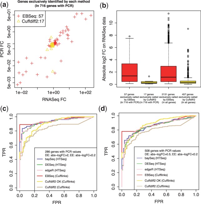
Panel (a) shows the fold changes (log₂ scale) from RNA-seq versus PCR for the 57 genes identified by EBSeq but not Cuffdiff2 and the 17 genes identified by Cuffdiff2 but not EBSeq out of the 716 gold-standard genes from the MAQC dataset. Panel (b) shows box plots of the absolute value of RNA-seq fold changes (log₂ scale) for the same 57 and 17 genes, as well as the 2131 and 457 genes identified exclusively by EBSeq and Cuffdiff2, respectively, in the full set of genes. Panel (c) shows ROC curves for baySeq, DESeq, edgeR, Cuffdiff2 and EBSeq. Cuffdiff2 and EBSeq are applied to gene expression estimated via Cufflinks. Results from EBSeq applied to gene expression counts derived from HTSeq are similar (data not shown). The ROC curves based on another threshold in Bullard et al. are shown in panel (d)

Panel (c) shows ROC curves for all methods derived using the same thresholds as in Bullard et al. (2010). Specifically, we define genes with an absolute value of log2 qRT-PCR fold change >2 as DE; genes with absolute value of log2 qRT-PCR fold change <0.2 are defined as EE. Using these thresholds, 286 of the 716 genes are classified as either DE (200) or EE (86). When the FPR is <20%, panel (c) shows that EBSeq performs best across all the methods; baySeq is slightly better than DESeq and edgeR, while Cuffdiff2 shows the lowest power. When FPR is >30%, baySeq, DESeq, edgeR, EBSeq and Cuffdiff2 (‘OK’) perform similarly. The ROC curves based on another threshold in Bullard et al. are shown in panel (d).

Each of the count-based methods was also applied to 100 Sim III datasets. Table 2 shows the power and FDR of each method at 5% target FDR averaged over the 100 simulated datasets. In short, all methods have well-controlled FDR. EBSeq shows the highest power (∼79%), with DESeq and edgeR showing comparable performance (∼73%), and although baySeq seems to outperform DESeq and edgeR with respect to ranking genes (as demonstrated in the ROC curves shown in Fig. 3c and d), it has lower power (∼61%) than both DESeq and edgeR when FDR is controlled at 5%. Section 4 of the Supplementary Material shows that FDR is affected by outliers. In particular, although the FDR of edgeR is well-controlled overall, simulation results suggest that the false calls that are made by edgeR are almost always in genes with outliers. The ROC curves averaging 100 Sim III datasets are shown in Supplementary Figure S10.

Table 2.

Gene simulation results

Methods	Power (%)	FDR (%)
baySeq	60.8	0.4
DESeq	73.4	0
edgeR	73.1	4.6
EBSeq	78.8	2.7

The empirical power and FDR of baySeq, DESeq, edgeR and EBSeq averaged across 100 Sim III simulations where target FDR was set at 5%. Standard errors on average power (FDR) were <2.5% (1.4%) and are not shown.

3.3 Case study of human embryonic stem cell lines

To further evaluate and compare methods, we analyse data from an experiment comparing human ES cell lines with iPS cell lines using DESeq, edgeR and baySeq (with expression counts obtained from HTSeq) as well as Cuffdiff2 (with expression estimated via Cufflinks). EBSeq is evaluated on both HTSeq- and Cufflinks-processed data. DESeq, edgeR, baySeq and Cuffdiff2 identify 127, 377, 34 and 54 DE genes at 5% FDR, respectively. EBSeq identifies 334 from HTSeq counts and 351 from Cufflinks estimated counts. These results are largely consistent with those observed in the simulation studies.

Recall that gene-level simulations and MAQC analysis demonstrate that EBSeq has slightly increased power over DESeq and edgeR; baySeq and Cuffdiff2 are underpowered compared with these other approaches; and all methods have well-controlled FDR. They also suggest that the false discoveries that are identified by edgeR are likely due to outliers. In the case study, EBSeq finds more genes than DESeq; baySeq and Cuffdiff2 find far fewer than either method; edgeR identifies most genes. As we have no gold standard in this case study, it is difficult to assess whether the genes identified exclusively by EBSeq (or edgeR) are the result of improved power (i.e. they are true discoveries) or an increased FDR. As we detail below, a close consideration of the genes identified exclusively by each method suggests that EBSeq shows improved power.

In particular, panels (a) and (b) of Figure 4 show the number of genes found by each approach. There are 114 genes found by DESeq, edgeR and EBSeq via HTSeq-processed data; 161 genes found exclusively by EBSeq (neither DESeq nor edgeR find these); and 197 found exclusively by edgeR (neither DESeq nor EBSeq find these). Figure 4c shows box plots of Dixon’s Q-statistics for these 114, 161 and 197 genes. As shown, the genes exclusively identified by edgeR tend to have higher Dixon’s Q-statistics, and are therefore more likely to contain outliers. Of course a gene may contain an outlier and still be DE. To assess this possibility, Figure 4d considers how a gene’s fold change changes when its most extreme value is removed, as quantified by the FCRatio. If a gene’s most extreme value is not largely responsible for the DE call, fold changes with and without the value will remain largely unchanged, and FCRatio will be near one (see Section 2). As shown, edgeR tends to favour genes with FCRatios far from 1, suggesting that the genes identified may be due to a single outlier in an otherwise EE gene. Supplementary Figure S11 shows nine genes identified exclusively by edgeR having highest Dixon’s Q-statistic. Many of the genes appear to be EE with a single outlier, and all of them have very low counts. Figure 4e shows the box plots of each gene’s 75th percentile of expression in the groups of 114, 161 and 197 genes. The genes identified exclusively by edgeR have lower expression on average than the other groups while the genes identified exclusively by EBSeq tend to be highly expressed. Figure 4f shows the CDFs of each gene’s 75th percentile of expression in the groups identified by each of the five methods. Approximately 20% of the genes identified by edgeR are with 75th percentile of expression <20.

Fig. 4.

Results are shown for the human embryonic stem cell case study, which compares ESCs with iPSCs. Panel (a) shows a Venn diagram of the genes identified as DE by DESeq, edgeR or EBSeq using HTSeq for quantification. Panel (b) shows a Venn diagram of the genes identified by Cuffdiff2 and EBSeq using Cufflinks-processed data. Panel (c) shows box plots of Dixon’s Q-statistics in three groups of genes—the 114 identified by DESeq, edgeR and EBSeq; the 161 identified by EBSeq but not DESeq or edgeR; and the 196 identified by edgeR but not DESeq or EBSeq. Panel (d) shows the FCRatios and Dixon’s Q-statistics of the genes identified exclusively by each method, but not the other four methods (in this panel, five methods are compared). Note that baySeq, Cuffdiff2, DESeq, edgeR and EBseq (via HTSeq) identify 34, 54, 127, 377 and 334 DE genes, respectively, at 5% FDR. Panel (e) shows box plots of each gene’s 75th percentile of expression for the three groups of genes defined in panel (c). Panel (f) shows the CDF of the 75th percentile of expression among the 34, 54, 127, 377 and 334 DE genes identified by each method

Results from the gene and isoform comparisons between EBSeq and Cuffdiff2 via Cufflinks-processed data are also consistent with the simulation study, with Cuffdiff2 identifying far fewer genes and isoforms than EBSeq. Specifically, Cuffdiff2 identifies seven isoforms, each of which is identified by EBSeq, but EBSeq also finds additional isoforms to be DE (935 in total). Furthermore, in this case study, isoform-level results obtained from EBSeq are more consistent with gene-level results than those obtained from Cuffdiff2. Specifically, there are 12 404 single-isoform genes. For these, we expect isoform and gene-level inference to match (i.e. if the isoform is DE, the gene should also be DE, given there is only a single isoform in that gene). Of the 54 genes identified as DE by Cuffdiff2, 39 have single isoforms; only 5 of the 39 are also identified as DE isoforms by Cuffdiff2. Of the 351 genes identified as DE by EBSeq, 226 have single isoforms and 225 of the 226 are also called DE at the isoform level by EBSeq. Furthermore, many important genes confirmed to be DE between ESCs and iPSCs in previous studies (Bock et al., 2011; Ohi et al., 2011; Phanstiel et al., 2011) are missed by Cuffdiff2 but not EBSeq, including DPP6, FAM19A5, SOX17 and DNAJC15.

4 CONCLUSIONS

The main difference between EBSeq and the other approaches considered here is that EBSeq models isoform expression directly, as opposed to gene expression, and in so doing accommodates isoform expression-estimation uncertainty. In particular, estimation uncertainty is partitioned into three groups defined by isoform complexity ( or 3), following our empirical observation that uncertainty is increased on average in isoforms that share a parent gene. EBSeq is not restricted to three groups, and for some genomes, additional I_g groups may be warranted. EBSeq is also not restricted to this definition of complexity (see Implementation below). EBSeq shows increased power over Cuffdiff2 for identifying DE isoforms. Although developed to facilitate isoform inference, like Cuffdiff2, EBSeq may also be used for identifying DE genes. It shows slightly increased power over most count-based methods in both simulation and case studies, without major losses in efficiency when outliers are present.

A second difference is that, unlike most approaches that classify non-DE genes as EE, EBSeq is based on a parametric mixture model, which facilitates evaluation of the posterior probabilities associated with DE, as well as EE. The particular parameterization provides closed form predictive distributions that facilitate efficient computation. However, diagnostics should always be checked to ensure model fit (see Section 7 of the Supplementary Material). Once posterior probabilities are obtained from a well-fit model, a user may identify an FDR-controlled list of EE genes. This may be of particular interest for genes with more than one isoform, as compensatory mechanisms may give rise to DE isoforms in EE genes, and consequently subtle, yet important, differences may be missed if focus is placed exclusively on DE genes alone. Using the EE posterior probabilities from the case study, EBSeq identified 64 EE genes, with DE isoforms contributing at least 30% of the gene expression (20 are shown in Supplementary Fig. S13). The mixture model framework also enables comparisons of more than two biological conditions (see Section 6 of the Supplementary Material).

5 IMPLEMENTATION

EBSeq is implemented as an R package (R Development Core Team, 2009), currently available at http://www.biostat.wisc.edu/∼kendzior/EBSEQ/ and soon to be available on Galaxy. EBSeq requires estimates of isoform expression, estimates of gene expression, or gene counts, but it is not specific to any particular estimation method.

For users that prefer RSEM (Li et al., 2010) for expression estimation, an EBSeq-RSEM pipeline has been developed so that a user may easily apply RSEM to quantify expression and then EBSeq to identify DE genes and isoforms. For well annotated genomes, where isoforms and their corresponding parent genes are well defined, a user may choose to quantify isoform complexity using three groups defined by I_g, as we have done here. For genomes that are not well annotated (e.g. for de novo assembled transcriptomes), a user could use another measure of isoform complexity. The RSEM-EBSeq pipeline takes reads’ unmappability scores and applies a K-means algorithm to cluster the isoforms into K uncertainty groups; the number of groups (K) defaults to 3. The unmappability scores are also provided as output and, consequently, a user could easily apply a K-means algorithm with different values of K or apply another clustering algorithm to define the uncertainty groups. Extensions that allow for continuous covariates and accommodate ordered conditions (e.g. time course data) are underway.

REFERENCES

- Anders S, Huber W. Differential expression analysis for sequence count data. Genome Biol. 2010;11:R106. doi: 10.1186/gb-2010-11-10-r106. [DOI] [PMC free article] [PubMed] [Google Scholar]
- Anders S, et al. Detecting differential usage of exons from RNA-seq data. Genome Res. 2012;22:2008–2017. doi: 10.1101/gr.133744.111. [DOI] [PMC free article] [PubMed] [Google Scholar]
- Bock C, et al. Reference maps of human ES and IPS cell variation enable high-throughput characterization of pluripotent cell lines. Cell. 2011;144:439–452. doi: 10.1016/j.cell.2010.12.032. [DOI] [PMC free article] [PubMed] [Google Scholar]
- Bullard JH, et al. Evaluation of statistical methods for normalization and differential expression in mRNA-seq experiments. BMC Bioinformatics. 2010;11:94. doi: 10.1186/1471-2105-11-94. [DOI] [PMC free article] [PubMed] [Google Scholar]
- Consortium M. The microarray quality control (MAQC) project shows inter- and intraplatform reproducibility of gene expression measurements. Nat. Biotechnol. 2006;24:1151–1161. doi: 10.1038/nbt1239. [DOI] [PMC free article] [PubMed] [Google Scholar]
- Dempster A, et al. Maximum likelihood from incomplete data via the EM algorithm. J. R. Stat. Soc. 1977;39:1–38. [Google Scholar]
- Dixon WJ. Analysis of extreme values. Ann. Math. Stat. 1950;21:488. [Google Scholar]
- Du J, et al. IQSeq: integrated isoform quantification analysis based on next-generation sequencing. PLoS one. 2012;7:e29175. doi: 10.1371/journal.pone.0029175. [DOI] [PMC free article] [PubMed] [Google Scholar]
- Glaus P, et al. Identifying differentially expressed transcripts from RNA-seq data with biological variation. Bioinformatics. 2012;28:1721–1728. doi: 10.1093/bioinformatics/bts260. [DOI] [PMC free article] [PubMed] [Google Scholar]
- Hardcastle TJ, Kelly KA. baySeq: empirical bayesian methods for identifying differential expression in sequence count data. BMC Bioinformatics. 2010;11:422. doi: 10.1186/1471-2105-11-422. [DOI] [PMC free article] [PubMed] [Google Scholar]
- Howard BE, Heber S. Towards reliable isoform quantification using RNA-seq data. BMC Bioinformatics. 2010;11(Suppl. 3):S6. doi: 10.1186/1471-2105-11-S3-S6. [DOI] [PMC free article] [PubMed] [Google Scholar]
- Jiang H, Wing WH. Statistical inferences for isoform expression in RNA-seq. Bioinformatics. 2009;25:1026–1032. doi: 10.1093/bioinformatics/btp113. [DOI] [PMC free article] [PubMed] [Google Scholar]
- Katz Y, et al. Analysis and design of RNA sequencing experiments for identifying isoform regulation. Nat. Methods. 2010;7:1009–1015. doi: 10.1038/nmeth.1528. [DOI] [PMC free article] [PubMed] [Google Scholar]
- Langmead B, et al. Ultrafast and memory-efficient alignment of short DNA sequences to the human genome. Genome Biol. 2009;10:R25. doi: 10.1186/gb-2009-10-3-r25. [DOI] [PMC free article] [PubMed] [Google Scholar]
- Li B, Dewey CN. RSEM: accurate transcript quantification from RNA-seq data with or without a reference genome. BMC Bioinformatics. 2011;12:323. doi: 10.1186/1471-2105-12-323. [DOI] [PMC free article] [PubMed] [Google Scholar]
- Li B, et al. RNA-seq gene expression estimation with read mapping uncertainty. Bioinformatics. 2010;26:493–500. doi: 10.1093/bioinformatics/btp692. [DOI] [PMC free article] [PubMed] [Google Scholar]
- Nicolae M, et al. Estimation of alternative splicing isoform frequencies from RNA-seq data. Algorithms Mol. Biol. 2011;6:9. doi: 10.1186/1748-7188-6-9. [DOI] [PMC free article] [PubMed] [Google Scholar]
- Ohi Y, et al. Incomplete DNA methylation underlies a transcriptional memory of somatic cells in human IPS cells. Nat. Cell. Biol. 2011;13:541–549. doi: 10.1038/ncb2239. [DOI] [PMC free article] [PubMed] [Google Scholar]
- Phanstiel HP, et al. Proteomic and phosphoproteomic comparison of human ES and IPS cells. Nat. Methods. 2011;8:821–827. doi: 10.1038/nmeth.1699. [DOI] [PMC free article] [PubMed] [Google Scholar]
- R Development Core Team. R: A language and environment for statistical computing. Vienna, Austria: R Foundation for Statistical Computing; 2009. [Google Scholar]
- Robinson MD, Oshlack A. A scaling normalization method for differential expression analysis of RNA-seq data. Genome Biol. 2010;11:R25. doi: 10.1186/gb-2010-11-3-r25. [DOI] [PMC free article] [PubMed] [Google Scholar]
- Robinson MD, Smyth GK. Moderated statistical tests for assessing differences in tag abundance. Bioinformatics. 2007;23:2881–2887. doi: 10.1093/bioinformatics/btm453. [DOI] [PubMed] [Google Scholar]
- Sandmann T, et al. The head-regeneration transcriptome of the planarian Schmidtea mediterranea. Genome Biol. 2011;12:R76. doi: 10.1186/gb-2011-12-8-r76. [DOI] [PMC free article] [PubMed] [Google Scholar]
- Singh D, et al. FDM: a graph-based statistical method to detect differential transcription using RNA-seq data. Bioinformatics. 2011;27:2633–2640. doi: 10.1093/bioinformatics/btr458. [DOI] [PMC free article] [PubMed] [Google Scholar]
- Smith CW, et al. Alternative splicing in the control of gene expression. Annu. Rev. Genet. 1989;23:527–577. doi: 10.1146/annurev.ge.23.120189.002523. [DOI] [PubMed] [Google Scholar]
- Stamm S, et al. Function of alternative splicing. Gene. 2005;344:1–20. doi: 10.1016/j.gene.2004.10.022. [DOI] [PubMed] [Google Scholar]
- Trapnell C, et al. Tophat: discovering splice junctions with RNA-seq. Bioinformatics. 2009;25:1105–1111. doi: 10.1093/bioinformatics/btp120. [DOI] [PMC free article] [PubMed] [Google Scholar]
- Trapnell C, et al. Transcript assembly and quantification by RNA-seq reveals unannotated transcripts and isoform switching during cell differentiation. Nat. Biotechnol. 2010;28:211–215. doi: 10.1038/nbt.1621. [DOI] [PMC free article] [PubMed] [Google Scholar]
- Trapnell C, et al. Differential gene and transcript expression analysis of RNA-seq experiments with TopHat and Cufflinks. Nat. Protoc. 2012;7:562–578. doi: 10.1038/nprot.2012.016. [DOI] [PMC free article] [PubMed] [Google Scholar]
- Trapnell C, et al. Differential analysis of gene regulation at transcript resolution with RNA-seq. Nat. Biotechnol. 2013;31:46–53. doi: 10.1038/nbt.2450. [DOI] [PMC free article] [PubMed] [Google Scholar]
- Wang ET, et al. Alternative isoform regulation in human tissue transcriptomes. Nature. 2008;456:470–476. doi: 10.1038/nature07509. [DOI] [PMC free article] [PubMed] [Google Scholar]
- Zhou Y, et al. A powerful and flexible approach to the analysis of RNA sequence count data. Bioinformatics. 2011;27:2672–2678. doi: 10.1093/bioinformatics/btr449. [DOI] [PMC free article] [PubMed] [Google Scholar]
Associated Data
This section collects any data citations, data availability statements, or supplementary materials included in this article.