

Abstract
Neuroimage phenotyping for psychiatric and neurological disorders is performed using voxelwise analyses also known as voxel based analyses or morphometry (VBM). A typical voxelwise analysis treats measurements at each voxel (e.g. fractional anisotropy, gray matter probability) as outcome measures to study the effects of possible explanatory variables (e.g. age, group) in a linear regression setting. Furthermore, each voxel is treated independently until the stage of correction for multiple comparisons. Recently, multi-voxel pattern analyses (MVPA), such as classification, have arisen as an alternative to VBM. The main advantage of MVPA over VBM is that the former employ multivariate methods which can account for interactions among voxels in identifying significant patterns. They also provide ways for computer-aided diagnosis and prognosis at individual subject level. However, compared to VBM, the results of MVPA are often more difficult to interpret and prone to arbitrary conclusions. In this paper, first we use penalized likelihood modeling to provide a unified framework for understanding both VBM and MVPA. We then utilize statistical learning theory to provide practical methods for interpreting the results of MVPA beyond commonly used performance metrics, such as leave-one-out-cross validation accuracy and area under the receiver operating characteristic (ROC) curve. Additionally, we demonstrate that there are challenges in MVPA when trying to obtain image phenotyping information in the form of statistical parametric maps (SPMs), which are commonly obtained from VBM, and provide a bootstrap strategy as a potential solution for generating SPMs using MVPA. This technique also allows us to maximize the use of available training data. We illustrate the empirical performance of the proposed framework using two different neuroimaging studies that pose different levels of challenge for classification using MVPA.
Keywords: Classification, Regression, Voxel Based Morphometry, Multi-Voxel Pattern Analysis, Generalization Risk, Image Phenotyping, Penalized Likelihood, Linear Models
1 Introduction
Many neuroimaging studies are conducted with a priori hypotheses to be tested. Voxelwise analysis1 (henceforth referred to as VBM) is the most widely used framework for hypothesis testing in neuroimaging. In this framework, the measurements at each voxel (or region) are treated as outcome measures and are analyzed independently leading to a large number of univariate analyses. Depending on the study, these measurements could be any of the following: cortical thickness obtained using T1 weighted images, blood oxygen level dependent activations obtained using functional magnetic resonance imaging (fMRI), fractional anisotropy computed using diffusion tensor images (DTI), or the index of metabolic activity using positron emission tomography (PET). The relationship between the outcome measure and the experimental design variables is commonly modeled using generalized linear models (GLM) of which the linear model (LM) is a special case (McCullagh and Nelder, 1989).2
With increasingly large amounts of data being collected, hypothesis testing alone fails to utilize all of the information in the data. Such studies may also be used to discover interesting patterns of regularity and to find image phenotypical information effecting individual differences in diagnosis, prognosis, or other non-imaging observations. Increasing sample sizes and multi-center studies combined with the maturation of high dimensional statistical tools has led to an increasing interest in multi-voxel pattern analysis (MVPA) (Norman et al, 2006; Pereira et al, 2009; Hanke et al, 2009a; Anderson and Oates, 2010; Carp et al, 2011; Halchenko and Hanke, 2010).3 Thus far, the majority of this work has been in the area of classification and primarily using functional magnetic resonance imaging in detecting various states of mind (Pereira et al, 2009). There is a growing interest, in the spirit of computer-aided diagnosis, in performing MVPA using structural information of the brain with modalities such as T1-weighted MRI and diffusion tensor imaging (DTI). However, performing MVPA using structural brain signatures is a harder problem than using functional brain signatures. This is because, except in studies investigating atrophy, structural changes (effect-sizes) are usually much smaller and reside in higher effective-dimensions compared to functional changes, thus demanding more data for both VBM and MVPA models. Yet, surprisingly, the majority of the neuroimaging studies have significantly more functional data collected compared to the structural data such as DTI. Hence, driven by improving performance scores such as cross-validation accuracies and area under the receiver operating characteristic (ROC) curves, the current research has primarily focused on the following two areas. (1) The first area involves developing pre-processing methods for extracting various features such as using topological properties of the cortical surfaces (Pachauri et al, 2011), spatial frequency representations of the cortical thickness (Cho et al, 2012), shape representations of region-specific white matter pathways (Adluru et al, 2009) or including various properties of the diffusion tensors in specific regions of interest (Lange et al, 2010; Ingalhalikar et al, 2011). Recent work in this direction has even been in performing meta analyses using large scale data from the published articles on the web for extracting specific regions in the brain relevant for a given task in fMRI studies (Yarkoni et al, 2011; Mitchell, 2011). (2) The second area involves developing various classifier models such as multi-kernel, multi-modal learning (Hinrichs et al, 2011; Batmanghelich et al, 2011; Zhang et al, 2012), incorporating spatial constraints to a linear program based boosting model (Hinrichs et al, 2009) and even ensemble classifier models (Liu et al, 2012).
However not much attention has been paid to analyzing the model-behavior beyond the basic metrics such as average cross-validation accuracy and ROC curves, except for a few upcoming articles such as Hinrichs et al (2011); Ingalhalikar et al (2011), which attempt to interpret the classifier model parameters and prediction scores. Although this is promising, to our best knowledge, there has been virtually no work conducted in careful risk assessment of such models in neuroimaging studies by employing generalization risk theory available in the statistical machine learning literature.
This paper has four main goals: (1) to unify the key aspects of the two main families of neuroimage analysis, VBM and MVPA by using penalized likelihood modeling (PLM); (2) to illustrate the fundamental differences of VBM and MVPA in terms of model selection and risk assessment and introduce practical generalization risk bounds using results from statistical learning theory; (3) to demonstrate that for obtaining statistical parametric maps (SPM) using MVPA, one faces an issue similar to the multiple comparisons problem; and (4) to show that there are critical conceptual level differences between the use of MVPA in artificial intelligence applications and neuroimaging studies, including differences between the challenges in state-detection (diagnosis) vs. trait-prediction (prognosis). We use DTI data from two neuroimaging studies to illustrate the potential of the proposed approach. The first study investigates the role of white matter in the autism spectrum disorders. The second study addresses the question of white matter plasticity effects of long-term meditation practice. We would like to note that PLM is not new to neuroimaging and has been used in the form of sparse regression by applying the ℓ1 penalty (Carroll et al, 2009; Vounou et al, 2010; Ryali et al, 2010; Bunea et al, 2011). However, to our best knowledge, our work is the first to use PLM in a global context for unifying VBM and MVPA, which enables us to provide better contrast between and comparison of the two families of analysis.
The remainder of the article is organized as follows. Section 2 contains materials and methods. Specifically, the mathematical and statistical concepts of penalized likelihood and risk assessment for both VBM and MVPA are presented in Sections 2.1, 2.2 respectively. Section 2.3 presents the neuroimaging data sets discussed in this paper and Section 2.4 describes the statistical hypotheses that are examined in connection to the proposed penalized likelihood phenotyping. The experimental results are presented in Section 3. Section 4 contains a discussion of the presented work and directions for future research in related areas. The Appendix presents an alternative approach for risk-assessment of MVPA, specifically derived for support vector machines.
2 Materials and Methods
In this section, we first describe how penalized likelihood modeling can provide a unified framework for voxel based morphometry (VBM) and the multi-voxel pattern analyses (MVPA) in the Section 2.1. We then explain how the models can be assessed and interpreted via risk assessment in Section 2.2.
2.1 Loss and Penalty
Penalized likelihood modeling (PLM), and more generally regularization, is rooted in the idea of inducing some selection bias for selecting parsimonious models in explaining the data, without much loss in estimation performance. To set the notation, let us assume we collect brain data (v number of voxels) and clinical covariates (p variables) on n subjects. Typically, in an imaging data set v ≈ 105, n ≈ 102, and p ≈ 10. For instance, in our autism study we have v = 41, 011, n = 154 and p = 4 (Age, Group, Social Responsiveness Scale (SRS), IQ). For the meditation study, we have v = 57019, n = 49 and p = 3 (Group, Age and Total Life Time Practice Hours (TLPH)).
We now explain how the data are modeled in VBM and classification, which is a canonical example in MVPA. VBM fits the following regression model at each voxel
| (1) |
Y is the vector of outcome measures observed in the brain, X is the design matrix of the p clinical variables and a column of constants, and β is a vector indicating the effect of each variable on the signal. The error term (ε) is assumed to follow the standard normal distribution, i.e. ε ~
 (0, 1). In contrast, consider the classification problem where the data are typically modeled as
| (2) |
In this setting, X is a matrix of vectorized brain signals also commonly known as the feature matrix. Y is the diagnostic or group-label information. Here, each brain is treated as a high-dimensional vector. Hence, a key difference between VBM and classification in data modeling is in the size of β. Specifically, in the classification setting β is a high-dimensional object (v ≫ n), while in the VBM setting it is not (p ≪ n). In addition to classification which translates to computer aided diagnosis, one can also model a high-dimensional regression in MVPA where Y ∈ ℝn×1. Such an MVPA regression model translates to computer aided prognosis4.
The key idea behind estimating such models, for both VBM and MVPA, is to balance data fidelity (using a loss/fitness function) and over-fitting (using a penalty). We would like to quickly note that over-fitting of a model should not be confused with precise estimation of a model. Precise estimation can lead to over-fitting when the model chosen a priori is not a complete description of the “reality” under consideration. Hence the goal under PLM, is to estimate the respective model parameters β by minimizing
| (3) |
where L is a loss function, P is a penalty which controls the complexity of the model, and λ ≥ 0 is a tuning parameter which controls the amount of penalization. This parameter can be thought to reflect the uncertainty in modeling the reality: smaller values reflect more confidence in the modeling. Typically, the loss function can be viewed as a negative log-likelihood of the model, hence the objective function in (3) is commonly known as a penalized likelihood function. Naturally different combinations of loss and penalty would result in different biases, optimization challenges and model behaviors. In VBM, the most commonly implemented loss function in popular neuroimaging packages such as SPM, AFNI, FSL, SurfStat, fMRIStat, is the following ordinary least squares (OLS) loss
| (4) |
Let us take a closer look at the above loss function. If we expand and re-group the terms, it can be upper bounded by
| (5) |
we can notice that the OLS loss function has an implicit penalty on ||β||2. Of course one could introduce additional penalty to the OLS resulting in for example, ridge regression (Marquardt and Snee, 1975). We can also use other robust loss functions such as the ε-insensitive ℓ1-loss function in combination with a ||β||1 as penalty (Adluru et al, 2012). The ε-insensitive ℓ1-loss used in the popular support-vector regression (SVR) is defined as
| (6) |
This loss-penalty combination also is very useful for computer-aided prognosis in the class of MVPA. In the Table 1, below we present some commonly used loss and penalty combinations in the family of VBM and MVPA. Different loss and penalty functions require different optimization routines to estimate β. For example, OLS has a closed form solution of β̂=(XTX)−1 XTY. Fortunately, the other combinations in the Table 1 are convex and computationally tractable and the optimization details have been analyzed, implemented and improved over time (Park and Hastie, 2007; Hastie et al, 2009; Friedman et al, 2010; Yuan et al, 2011).
Table 1.
Different loss-penalty combinations resulting in different types of models which fall under either VBM or MVPA. Such a penalized likelihood modeling point of view allows us to tie the two families of analysis into a unified analytic framework. This will also allow to us compare and contrast the differences and similarities in a principled way. Yi and Xi denote the group label and the vectorized brain image of the ith sample respectively. ||β||\0|| denotes the set of βs without the first coefficient β0, also known as bias.
| L (Y, Xβ) | λP(β) | Family | |||
|---|---|---|---|---|---|
|
| |||||
| ℓ2-SVM |
|
|
MVPA | ||
| ℓ1-SVM |
|
||β||1 | MVPA | ||
| ℓ1-logistic regression |
|
||β||1 | VBM and MVPA | ||
| OLS |
|
|
VBM | ||
| Ridge |
|
|
VBM and MVPA | ||
| SVR | |Y−Xβ|ε |
|
VBM and MVPA | ||
We would like to note that typically in MVPA models, each brain image is vectorized and treated as a single high-dimensional vector (as shown in Eq. (2)), that is the 3D volume structure of the brain scans is ignored. Hence the most commonly used penalties (shown in the Table 1 above) are vector norms such as ||β||1, ||β||2. Such vector norms take into account the high-dimensionality issue by taking into account the first order interactions but not products between different βis.
However one can devise classification models by keeping the full 3D volume structure of the brain images and treating them as tensors5, so that higher-order interactions between the βis can be accounted for in the norms. Such interactions might very well be relevant for analyzing patterns in these data. Tensors offer much richer variety of operations but for simplicity of understanding one can model the data for ith sample as
| (7) |
and vx, vy, vz are the number of voxels in the three directions. 〈·, ·〉 denotes the tensorial dot product which numerically is identical to vector dot product by vectorizing the two tensors (Signoretto et al, 2011). The main advantage of such tensorial view comes from the ability to add structural norms such as the Frobenius norm ( ), rank, Schatten {p, q}-norms (||β||p,q) or nuclear p-norms (||β||p,1), whose definitions using advanced singular value decompositions of tensors can be found in Kolda and Bader (2009); Signoretto et al (2011). Penalizing with some of these norms (Frobenius, nuclear 1-norm) has convex optimization routines while with some others (Schatten {p, q}-norms with p < 1) is computationally hard. Furthermore justifying these norms would require stronger a priori assumptions on the 3D structures of the βis such as having low-rank or other spectral-gap related assumptions.
Some such ideas have been applied in 2D natural image analysis such as face and gait detection by treating images as matrices and image sequences as tensors rather than vectors (Wolf et al, 2007; Kotsia et al, 2012), in tensor classification for online learning (Shi et al, 2011). Tensorial extensions have also been proposed for independent component analyses in brain fMRI analyses (Beckmann and Smith, 2005). But since the main goals of this manuscript are to unify the VBM and MVPA and present novel risk analysis approaches for the estimated models regardless of the loss-penalty combination, our experimental results focus on the most commonly used combinations (such as the ones presented in Table 1) and focus on test-set bounds and cost-function based examination of the ROC curves.
2.2 Risk Assessment
In the previous section we saw how penalized likelihood modeling helps us unify the models explored in VBM and MVPA as different combinations of loss and penalty in different vector (or possibly tensor) spaces. One of the key distinctions between VBM and MVPA will arise in the risk assessment of the estimated models. In each setting there are two-levels of risk assessment that correspond to performance and interpretation. These are summarized in Table 2 and will be described in detail in the following text.
Table 2.
Summarization of the two levels of risk assessment in VBM and MVPA. The key technology needed for each level is shown in the brackets. In both VBM and MVPA, these two levels can sometimes be jointly addressed for example, multivariate hypothesis testing (Kanungo and Haralick, 1995) in VBM and LASSO type loss-penalty combinations that allow simultaneous variable selection and model estimation (Tibshirani, 1996) in MVPA.
| Level | VBM | MVPA |
|---|---|---|
| 1st | Individual voxel level (type I error control via tail bounds) | Joint set of voxels (prediction error control via deviation bounds) |
| 2nd | Joint set of voxels (multiple comparisons) | Individual voxel level (variable selection) |
Voxel Based Morphometry (Level 1 Risk)
In VBM, the model selection process is based on domain specific knowledge. First, a certain set of null and alternate hypotheses are formulated. Then after identifying a set of variables of interest and potential nuisance variables, a control experiment is conducted to collect the data by randomizing on the nuisance variables. Power analysis (Mumford and Nichols, 2008) is usually (but not always and frequently enough) performed to calculate the amount of data that needs to be collected in order to be able to confidently reject the formulated null-hypotheses. Hence the focus of risk assessment is more on false rejection of null-hypotheses and less on model selection, interpretation and generalization. This a priori model selection, preferably based on other non-imaging data, results in a clear notion of outcome measures (dependent variables) and experimental design measures (independent variables). As discussed in Section 1, the relationship between dependent and independent variables is typically modeled as a linear model (LM).
A fixed LM is estimated using OLS (Eq. (4)) with data from each voxel and the risk of false-rejection of null-hypothesis at a voxel is based on a test statistic such as a p-value. The p-value is characterized by a tail bound on a null-distribution which typically is a student-t, F or χ2 distribution in asymptotics. The assumptions of asymptotic behavior are expected to be satisfied with sufficient number of samples. Generally one wants to test if a linear combination of the βs is statistically significant. That is, at each voxel, the following hypothesis testing is performed
| (8) |
where H0,i, H1,i are the null and alternate hypotheses respectively at ith voxel and
 is an m × p matrix typically called a contrast matrix. This method of using contrast matrices provides a general way of representing null-hypotheses. To assess the risk of false-rejection of the null hypotheses, we need to compute the following null-conditioned probability as the test-statistic
| (9) |
The null-hypotheses can then be rejected with at least 1 − α confidence level or at most α risk, if . Typically α is set to 0.05 in practice for various legendary and empirical reasons. Below show how Eq. (9) is computed typically using p-values. Let
| (10) |
| (11) |
β̂ denotes the estimated β using the data. Now, under the asymptotic and standard normality of residuals assumptions
| (12) |
| (13) |
where df = n − rank(X), is the degrees-of-freedom parameter for the two distributions. Thus t-distribution can be used if we rely on the precision in the estimated parameters and χ2 distribution can be used if we rely on the residuals of the estimated models. Assuming the above t and χ2 are the null-distributions, the probability of false rejection can then be computed as
| (14) |
where
| (15) |
| (16) |
and ft and fχ2 are the probability density functions for the t and χ2 distributions respectively. Testing significance of contrasts of βs using residuals involves using ratios of residuals of nested models resulting in F-tests (please see Adluru et al (2012) for examples and details). Adluru et al (2012) also show that more effective (data-driven) definitions of the df can be used to obtain better sensitivity in rejecting the null-hypotheses.
Thus the first level of risk assessment in VBM involves computing the p-values using a test statistic such as t0, or F0 and comparing those with α, at each voxel. The collection of the test-statistics at each voxel results in the so called statistical parametric maps (SPMs) which form the basis for image based phenotyping in the brain.
Image Phenotyping using VBM (Level 2 Risk)
The second level of risk arises because we will have tested v hypotheses (one at each voxel) in order to produce an SPM. To control the overall risk (also known as family wise error (FWER) control) we need to control
| (17) |
Although the risk at individual voxel level can be controlled by computing p-values, the joint probability is typically very hard to compute exactly since it is hard to know the interactions between the hypotheses explicitly. But assuming there is α risk of false-rejection at each voxel, it can be upper bounded using the union bound as
| (18) |
This upper bound, which is well known as Bonferonni bound or Boole’s inequality, says that the risk of false-rejection is linearly inflated with the number of hypothesis tests in a given experiment. This bound can be very loose in many neuroimaging studies and tends to be overly conservative. One can also use the following (slightly tighter) inequality, based on De Morgan’s law, also commonly known as Sídak bound
| (19) |
Naturally α ≤ 1 − (1 − α)v ≤ αv for α ∈ (0, 1]. Hence to control for false rejections with at most α risk at the family level (17), we need to control the individual voxel level risk much more strictly. Specifically as follows,
| (20) |
We can also observe that if is not controlled at low values, the bounds would be trivial and practically un-useful. For instance, they would result in statements such as the family-wise risk is less than 1.0 and 2500 at α = 0.05, v = 50000 when applying Eqs. (19) and (18), respectively6. Such methods however do not take into account the amount of spatial smoothing performed on Y or smoothness present in the SPMs. From Eq. (14), we can see that essentially involves computing probabilities like P (ξ0,i ≷ x), where ξ0,i is the test statistic at ith voxel in the SPM. By treating an SPM as a random field, the Eq. (17) can be approximated using random field theory (RFT) as follows (Worsley et al, 2004; Taylor and Worsley, 2008)
| (21) |
where Reselsd are the resels (resolution elements) of the search region (S) and ECd is the Euler characteristic density of the excursion set of the SPM (thresholded SPM) in d dimensions. The expressions for these can be found in Worsley et al (1996). We use the implementations are available in the SurfStat software package (Worsley et al, 2009) in our experiments. The RFT correction is very similar in spirit and in fact can be used to motivate the cluster-based corrections (Smith and Nichols, 2009). Permutations-based correction (Nichols and Holmes, 2002) controls the overall risk by Monte-Carlo simulations of the null-distributions rather than assuming any parametric form (such as t, χ2 or F) for them or clusterwise thresholding of the test statistics in the SPM. Finally, instead of controlling FWER one can also control for proportions of false rejections also known as false discovery rate (FDR) control (Benjamini and Hochberg, 1995).
The key thing to be observed is that the multiple comparisons issue in VBM arises mainly when trying to obtain image phenotyping information by controlling the overall risk of false-rejection of null-hypotheses at the neuroanatomical level. Furthermore, predictions at an individual subject level is not a concern in VBM hence there is no explicit assessment of generalization of the model performance on “unseen” or “uncollected” data.
Multi-voxel Pattern Analysis (Level 1 Risk)
As in the case of VBM there are two-levels of risk assessment in MVPA, except the treatment of the voxels is reversed as shown in Table 2. Here the data are typically not collected with a priori hypotheses as in the case of VBM. Hence the notion of independent and dependent measures is less clear and not relevant in this family of analyses. The idea is to discover flexible enough models, using already collected data, to be able to perform well on the future/unseen data. In VBM, either the precision of the estimated parameters or the residuals of the estimated models are used to assess the first level risk. Since the model selection is not performed a priori as in VBM and since p ≫ n, the risk assessment is necessarily different from that in VBM. The focus becomes more on generalization, model selection and interpretation, rather than testing to reject any null-hypotheses at an α risk level.
It is important to first understand some historical context of the MVPA in neuroimaging based neuroscience, for careful risk assessment of MVPA models. MVPA in neuroimaging studies is mainly an off-spring of machine learning models used primarily in imaging based artificial intelligence (AI) applications such as computer vision and robotics7. The goal in imaging based AI applications is fundamentally different from imaging based neuroscience applications. In the former, the goal is to endow machines with models that potentially mimic human capabilities such as object recognition, autonomous navigation and text classification. For example it is easy (easy to learn) for humans to walk around autonomously, summarize textual images, parse natural scenes. While in neuroimaging the goal of mimicking humans, except in specific degenerative cases like Alzheimer’s disease with gray matter atrophy and stroke, is ill-defined since it is essentially impossible (yet) for even an expert neuro-scientist to look at brain imaging data and decide, for example, whether a person has autism. Although theoretical work on assessing generalization risk in machine learning has been addressed by many researchers, the status-quo of many of the results are unsatisfactory in the practical setting leading to findings such as “generalization risk is less than 0.9” (Langford and Shawe-taylor, 2002)8. This is a less critical issue in human-mimicking AI applications, since in those applications one can have a strong control on the risk by having a human in the loop9.
There are several approaches one can take in analyzing the risk of an estimated multivariate model such as using probably approximately correct (PAC)-learnability (Valiant, 1984), defining the “capacity” or “effective dimensions/degrees of freedom” of the models using VC-theory (Vapnik and Chervonenkis, 1971), prediction error/mistake-bounds (Langford and Shawe-taylor, 2002), cross-validation based analysis (Kearns and Ron, 1999). Although these different frameworks are related to one another, we will mainly focus on employing the prediction error bounds. This is due to practical implications of the different approaches. The other frameworks are useful in general purpose understanding and designing models of MVPA. For example, SVM estimation can be interpreted as minimizing empirical risk, since the norm of the weights (||β||) is related to VC-dimension of the class of SVMs. However, the bounds using such analogy are either very loose are hard to compute in practice. Prediction error bounds on the other hand are easier to compute for practical application of the prediction theory (Kääriäinen and Langford, 2005). Hence we propose those as an extension to the routinely reported metrics such as average accuracies and receiver operating characteristic (ROC) curves.
The most commonly used cross-validation (either leave-one-out or k-fold) can provide a reasonable sense of the model performance but when computing the risk bounds, notions like algorithm stability and hypothesis stability come into play. We do not go into details of such results in this article but refer the interested readers to an excellent article (Kearns and Ron, 1999). We will however use the cross-validation data for dissecting the ROC curves to report confidence intervals of the true-positive rate (TPR) at various optimal operating regions (please see section 3 for details on this).
Before we introduce basic quantities needed to compute the prediction error bounds, we would like to highlight the difference between (1) MVPA regression models used for predicting continuous variables known in neuroscience as traits or individual differences or symptom severities, and (2) classification models used for predicting discrete variables called as state, class or group prediction. The notion of robustness, although can be defined using heuristics such as ℓ1 loss (Huber, 1981) in the case of trait prediction, can be more crisply captured in the state prediction using variants of the 0/1 loss (Valiant, 1984). This also amounts to additional challenges in risk assessment of the estimated models. Hence in this manuscript we will primarily focus on computing state prediction error bounds. With these bounds the risk that we are assessing, is on the underestimation of the errors made by the classifier models (false positiveness in prediction accuracies).
The empirical (or estimated) prediction error of an MVPA classifier model (β̂) on a test-set DTest, is defined as
| (22) |
Since we do not know parametric forms of the distribution of ε̂, the best we can hope for is to model its distribution using the hypothetical true prediction error defined as
| (23) |
where D is the “true” multivariate high-dimensional distribution from which the data is sampled.
The empirical error rate (ε̂) then follows a hypothetical (since ε is not known) binomial distribution of heads/tails of biased coin flips with a bias of ε
| (24) |
which characterizes the probability of observing k empirical errors in n predictions when the true error rate is ε. The tail probability, which is the probability of observing up to k errors in classification, can then be defined as
| (25) |
However since we do not have access to ε, we cannot compute the above probability exactly. In other words we do not know which binomial distribution the empirical error rate (ε̂) follows10. Hence the risk assessment is modeled as the probability of deviation of ε̂ from ε at a pre-determined confidence (1− α) or risk (α) levels.
Now, using standard properties of the binomial distribution one can obtain (Kääriäinen and Langford, 2005),
| (26) |
where
| (27) |
is the Binomial tail inversion representing the largest bias (true error rate), such that we can observe up to ε̂ in n prediction attempts, with at least α probability. This is known as the test-set upper bound which states that the chance of large deviation of true error above the tail inversion obtained using the test-set error rate, is bounded by α. Similarly a lower bound can be obtained as (Kääriäinen and Langford, 2005)
| (28) |
where
| (29) |
is the opposite of Eq. (27) reflecting the smallest bias, such that we can observe at least ε̂ errors i.e. ε̂ or more number of errors in n prediction attempts, with at least α probability. These upper and lower bounds can provide us binomial confidence intervals on the prediction error rates thus allowing us to state the following about the true error rate. With 1 − α confidence,
| (30) |
This is a tighter interval compared to the following interval that is sometimes reported in literature (assuming α ≤ 0.05),
| (31) |
where
Although at higher error rates binomial can approximate the normal distribution, for lower error rates (30) is tighter (tightest possible) compared to (31).
We now discuss the practical issues encountered when reporting (30). Computing this interval requires an independent test-set for evaluating the model. That is ε̂ has be to be replaced by
| (32) |
and n by ntest. In our experimental results we split the data into various training/test sets as shown in Table 4. In typical neuroimaging studies however, there is insufficient data for training multivariate models. Hence, researchers tend to use all of the data without holding an independent test set. Furthermore the test-set bounds are agnostic to the specific loss-penalty combination and work purely based on the mistakes made by the model. This naturally leads to a discussion of the so called training set bounds which can allow us to use all the available data as well as take into account specific class of the MVPA models. Classes of MVPA models are characterized by their “effective power” in prediction. The more powerful a class is the looser the training set bound would be, for a fixed amount of training data. One can draw an analogy to the degrees of freedom of a LM used in VBM, the larger the rank(X), the less are the df the power to reject a null-hypothesis, for a fixed α and n. The flip-side of taking class into account is that the bounds are derived for the families of classifier models rather than the specific learned/estimated model. Although there are techniques to “de-randomize” the bounds, from a data analysis perspective the focus in this paper is computing the test-set intervals (please see the numerical results for the two studies are reported in Section 3). Please see Section 4 and the Appendix for further discussion of the training set bounds for support vector machines.
Table 4.
Test-set bounds (Binomial confidence intervals) for various train/test splits for both neuroimaging studies. We can observe that in several of these attempts even when accuracy reaches beyond chance level, the bounds are quite loose, thus showing that one has to be careful in claiming generalization of the performance of the classification.
| Train/Test Proportions | Autism | Meditation |
|---|---|---|
|
| ||
| 90/10 | 56.25% [45.17 86.79] | 100% [0 54.93] |
| 80/20 | 70.97% [54.81 83.94] | 60% [30.35 85] |
| 70/30 | 63.83% [50.82 75.48] | 60% [35.96 80.91] |
| 60/40 | 72.58% [61.76 81.71] | 55% [34.69 74.13] |
| 50/50 | 62.34% [52.36 71.58] | 68% [49.64 82.97] |
Image Phenotyping using MVPA (Level 2 Risk)
The second level of risk assessment specifically involves the model selection rather than model performance although both can be addressed jointly in some situations as discussed in Table 2. Summarizing the model parameters (β) in the MVPA to produce a SPM is a challenging open problem. The main challenges that need to be addressed are (1) the fact that βis are estimated jointly and we need to take into account the inter-dependencies and (2) that the estimation is performed using disproportionately small amounts of data and hence the precision and stability in the estimated βis need to be carefully defined. A typical approach is to perform some basic normalization of the β̂is and define a significance threshold for declaring some of the voxels as critical. We take a more principled approach of computing z-scores for qualitatively approximating a significance map. Let be the average of the estimated parameter that corresponds to the voxel i across all cross-validation folds which serve as a bootstrap for the estimation. zi is then simply the normalized score defined as
| (33) |
where u and s are the functions for sample means and standard deviations. We can then work with the assumption zi ~
(0, 1) and can threshold for an appropriate α significance level. Note that although we do not explicitly face the multiple comparisons problem as in the case of VBM, we are still faced with another challenge of robust model selection using limited data known commonly as variable selection problem in statistics and machine learning communities. Some loss-penalty combinations, such as the LASSO (Tibshirani, 1996), induce sparse solutions and allow for simultaneous variable selection and parameter estimation. For more details we refer the reader to Bickel et al (2006), Hesterberg et al (2008), and Fraley and Hesterberg (2009).
2.3 Neuroimaging Data
We used data from two different neuroimaging studies. The first study investigates white matter substrates of autism spectrum disorders (ASD). The second study investigates the neuroplasticity effects of meditation practice on white matter. The sample characteristics of both the studies are presented in Table 3. Both studies used diffusion tensor imaging (DTI) data to investigate how white matter microstructure is affected. Briefly, DTI is a modality of magnetic resonance imaging that is exquisitely sensitive and non-invasively maps and characterizes the microstructural properties and macroscopic organization of the white matter (Basser et al, 1994; Jones et al, 1999; Mori et al, 2002). This is achieved by sensitizing MR signal to the diffusion of the water molecules (protons in them). Specifically the diffusion of the protons causes exponential attentuation in the signal proportional to their apparent diffusion coefficient (ADC) and the MR acquisition parameter known as b-value or b-factor (Le Bihan et al, 2001). That is S = S0e−bADC, where S is the measured MR signal, S0 is the signal without diffusion weighting or b = 0. The b-value represents the magnitude, duration, shape of the applied magnetic field gradients and time between the paired gradients used to flip the precessing protons and has units of seconds per square millimeters (s/mm2) (Le Bihan et al, 2001). By measuring the attenuated signal in atleast six different directions one can estimate the diffusion pattern of the protons in the three orthogonal Cartesian directions using a positive semi-definite covariance matrix also known as the diffusion tensor.
Table 3.
Sample characteristics such as sample sizes, gender distribution, means(standard deviations) of the continuous measures from the two studies. ASD stands for autism spectrum disorders group, TDC for typically developing controls group. LTM - long term meditators group, MNP - meditation näive practitioners group. TLPH - total lifetime practice hours. TLPH is computed using self-report measures of the number of retreats and number of hours at those retreats. Social Reciprocity/Responsiveness Scale (SRS) is a quantitative, dimensional measure of social functioning across the entire distribution from normal to severely impaired functioning (Constantino et al, 2000).
| Autism | Meditation | |||
|---|---|---|---|---|
|
| ||||
| Group | TDC (n = 55) | ASD (n = 99) | MNP (n = 26) | LTM (n = 23) |
|
|
||||
| Age | 15.25 (6.53) | 13.73 (8.94) | 49.7 (10.5) | 50.73 (9.9) |
| Gender | M=55, F=0 | M=99, F=0 | M=8, F=18 | M=9, F=14 |
|
|
||||
| IQ | 117.36 (15.30) | 93.57 (22.31) | N/A
|
|
| SRS | 16.12 (11.40) (n = 42) | 101.65 (27.89) (n = 94) | N/A | |
|
|
||||
| TLPH | N/A | N/A | 9602.8 (7979.7) | |
In the brain white matter, which consists of packed axon fibers, the diffusion of water is anisotropic, i.e., directionally dependent, because the movement of water molecules perpendicular to the axon fibers is more hindered than in the parallel direction. From the diffusion tensor one can obtain maps of the diffusion tensor trace, the three eigenvalues, anisotropy and orientation (direction of the largest eigen vector) (Basser and Pierpaoli, 1996). Various such measures from DTI have been used to characterize differences in brain microstructure for a broad spectrum of disease processes (e.g., demyelination, edema, inflammation, neoplasia), injury, disorders, brain development and aging, and response to therapy (Alexander et al, 2007). Fractional anisotropy (FA), the most commonly used measure of diffusion anisotropy, is a normalized standard deviation of the eigenvalues that ranges between 0 and 1. Although FA can be effected by many factors, empirically different studies have indicated that the higher the value, the more organized (in a primary direction) and the greater is the white matter integrity.
Autism Study
DTI data from a total of 154 male subjects were used in this study. The data were acquired on a Siemens Trio 3.0 Tesla Scanner with an 8-channel, receive-only head coil using a single-shot, spin-echo, echo planar imaging (EPI) pulse sequence and sensitivity encoding (SENSE) based parallel imaging (undersampling factor of 2). Diffusion-weighted images were acquired in twelve non-collinear diffusion encoding directions with diffusion weighting factor b = 1000s/mm2 in addition to a single reference image (b = 0). Other acquisition parameters included the following: contiguous (no-gap) fifty 2.5mm thick axial slices with an acquisition matrix of 128 × 128 over a field of view (FOV) of 256mm, 4 averages, repetition time (TR)=7000ms, and echo time (TE)=84ms.
Meditation Study
DTI data from 49 subjects were used in this study. The diffusion weighted images were acquired on a GE 3.0 Tesla scanner using 48 non-collinear diffusion encoding directions with diffusion weighting factor of b = 1000s/mm2 in addition to eight b = 0 images.
Image Pre-processing
For both the studies, eddy current related distortion and head motion of each data set were corrected using FSL software package (Smith et al, 2004). The brain region was extracted using the brain extraction tool (BET), also part of the FSL. Field inhomogeneity distortions were corrected using field maps acquired in the meditation study. The tensor elements were calculated using non-linear estimation using CAMINO11. It is important to establish spatial correspondence of voxels among all the subjects before performing VBM. State-of-the-art diffusion tensor image registration DTI-TK12 was used for spatial normalization of the subjects. It performs white matter alignment using a non-parametric, highly deformable, diffeomorphic (topology preserving) registration method that incrementally estimates its displacement field using a tensor-based registration formulation (Zhang et al, 2006).
Features
For MVPA models, extracting features from the DTI data can be very sophisticated. For example, Lange et al (2010) uses various diffusion tensor invariants such as FA in combination with other geometric properties in highly specific regions chosen a priori. While such efforts are extremely critical and useful for improving classification accuracies (Chu et al, 2012), we aim at keeping the features to be simple for two key reasons: (1) we have limited data to learn a classifier and by having a complex combination of features we risk generalizability; (2) we want to be able to interpret the features used in the classifier so that we can obtain image phenotypical information from the MVPA. In this study we perform both VBM and MVPA using fractional anisotropy (FA) in the white matter defined as the voxels with mean FA > 0.2 resulting in approximately 50000 voxels in each study. Furthermore, we restrict ourselves only to linear kernels, where the estimated parameters (learned weights) can be interpreted using z-scores. The data is smoothed for full-width half-maximum (FWHM) of Gaussian 4mm to account for mis-registrations during spatial normalization. Following the empirically chosen defaults from DTI-TK, the final set of spatially normalized images are resampled to 96 × 112 × 72 voxels with 2 × 2 × 2mm3 size per voxel. Hence, the FWHM 4mm smoothing roughly accounts for misalignment up to 1.5 voxels.
2.4 Hypotheses Examined
In this section, we present the hypotheses that are examined (estimated and tested for significance) for the penalized likelihood phenotyping i.e. VBM and MVPA. We would first like to note that the ‘addition of covariates’ approach is not a substitute to a clean randomization of a population study. In the case of VBM nuisance variables can lead to (a) either artificially reducing the sample size (by forcing to use only ‘controlled’ subset of the full sample) or (b) adding those variables into the models, both of which result in a reduction of statistical power of hypotheses testing essentially due to decrease in degrees of freedom of error. Furthermore finding a controlled sub-sample from the full-sample could be tricky because (1) there could be a large number of subsets to examine, (2) one has to either verify if the sub-samples follow known parametric distributions (such as normal) on the nuisance variables or perform permutation testing using each of the sub-division, and (3) one has to choose the subset that can maximize the statistical power. Satisfying all the three could be computationally very demanding.
Since in most realistic-population studies there always are a few nuisance variables and since choosing ‘controlled’ subsets is very challenging, addition of nuisance variables to the models is often used as a remedy. In the case of MVPA however, there is a stronger reason for not using only subsets of data. MVPA models are orders of magnitude higher in dimensionality compared to VBM models and larger models need more data for accuracy in estimation. Hence say by adding one or two nuisance variables to a model already containing 50,000 variables we can salvage about 100 samples, the cost to benefit ratio would be low at least in building an accurate predictive model.
Although fundamentally the idea of adding covariates into a model to control for the nuisance variables is similar in both VBM and MVPA, the control in MVPA is obtained at the phenotyping stage (using their relative importance compared to imaging covariates) and not in the predictive stage.
With these notes in mind, we examine the following set of hypotheses in the VBM category at each voxel in the white matter.
Autism Study (VBM Models)
-
Group effect on fractional anisotropy (FA). Here we test if the null-hypothesis that there is no difference in group-means of FA between autism spectrum disorders (ASD) group and typically developing control (TDC) group, can be rejected. Since the groups are not matched on IQ distributions, we regress out the effect of IQ on FA, the outcome measure in this case. The corresponding linear model (LM) can be expressed using MATLAB terms (Worsley et al, 2009) asFor experiments, we estimate the over-parameterized version of the above LM as
where ASD and TDC are the indicator variables. The contrast matrix used is
= [0 − 1 1 0], i.e. the null-hypothesis is
. -
Effect of Social Reciprocity/Responsiveness Scale (SRS) on FA. SRS is a quantitative, dimensional measure of social functioning across the entire distribution from normal to severely impaired functioning (Constantino et al, 2000). In this hypothesis we measure the effect of SRS on FA above and beyond IQ and Age. That is we want to measure how important SRS is in predicting FA in the context of using IQ and Age jointly. The corresponding LM is
The contrast matrix is
= [0 1 0 0], i.e. the null-hypothesis is β1 = 0. We test this hypothesis only using the ASD group (n = 93) since the variance in the measured SRS for the TDC group is limited.
Meditation Study (VBM Models)
-
Group effect on FA. In this hypothesis we are interested if the group-means of FA are different between long term meditation practitioners (LTM)s and wait-list controls (WL)s. The WL group sometimes is also referred to as meditation näive practitioners (MNP). The corresponding over-parameterized LM is
where LTM and WL are the indicator variables and the contrast matrix is
= [0 −1 1] representing the null-hypothesis
. -
Here we are interested in the neuroplasticity effect of meditation practice. Here meditation is conceptualized as a form of mental training cultivated for various ends, including emotional balanced and well-being. In the present study, meditators have been trained in standard Buddhist meditation techniques. These techniques lead to the cultivation of emotion regulation and attention control. The amount of formal meditation in life is used in the present study to interrogate the effect of meditation on the FA. Although this is cross-sectional data we can still hope to measure the effect of life time practice hours (TLPH) on the FA. TLPH is computed using self-report measures of the number of retreats and number of hours at those retreats. The corresponding LM is
and the contrast matrix is
= [0 1 0 0].
We estimate all of the above LMs using ordinary least squares loss implementation available in SurfStat (Worsley et al, 2009) and produce t-statistic maps.
Besides the VBM based hypotheses, we explore the following MVPA based hypotheses for phenotyping. We perform the following two types of MVPA: (1) classification, most commonly performed in the spirit of computer aided diagnosis; and (2) high-dimensional regression in the spirit of computer aided prognosis.
Autism Study (MVPA Models)
-
Here we ask the question of how well the FA in the white matter voxels jointly can predict the group label of an individual. The MVPA model for this can be expressed as
(34) Here the Group variable is treated as a binary variable. We include IQ in the model since the samples in the two groups are not perfectly matched for it and could be a predictive feature. We would like to highlight a key difference between the MVPA and VBM is that there is no explicit randomization performed on the model parameters when the data is being collected and hence the MVPA models are also known as “data-driven”. Hence, as discussed in the beginning of this section, to maximize the training data available we can be agnostic to the randomizations and can include such non-imaging parameters as well in these models. The z-score phenotyping will then show the relative importance of the imaging parameters as compared to such variables which are typically labeled as confounding or nuisance variables in VBM.
- We then examine if SRS in the ASD group can be predicted using white matter FA in the context of using IQ and Age as predictors. The corresponding MVPA model is
(35)
Meditation Study (MVPA Models)
The following correspondingly similar MVPA models are estimated
Group = β0 + β1FA1 + β2FA2 + … + βvFAv,
TLPH = β0 + β1FA1 + β2FA2 + … + βvFAv + βv+1Age + βv+2Gender.
We estimate the above multivariate models using support vector machine (SVM) and support vector regression (SVR) loss-penalty combinations (see Table 1). We use the implementations available via LIBSVM (Chang and Lin, 2001) and GLMNet (Friedman et al, 2010; Yuan et al, 2011). We report both the model performance as well as the image phenotyping information.
3 Experimental Results
In this section we will present and discuss the results of the models discussed in the previous section both for VBM and MVPA. Fig. 1 presents the distribution the t-statistics and the thresholds (FWER ≤ 0.05) based on Bonferonni correction and random field theory. We can observe that the t-statistics do not quite reach those correction thresholds. Hence we present the corresponding statistical parametric maps (SPMs) thresholded at a significance of α = 0.005 which is called “uncorrected” significance. Fig. 2 shows SPMs and sample cluster data in corpus callosum and brain stem from the VBM hypotheses examined in the autism study. Similar results for the meditation study are shown in Fig. 3. The corresponding figure captions provide more detailed discussions of these results.
Fig. 1.

Distribution of the voxelwise t-statistics on the four VBM hypotheses examined. The corresponding LMs are shown in the titles of the plots. The uncorrected, Bonferroni and random-field theory (RFT) based t thresholds at α = 0.005 and FWER ≤ 0.05 respectively, are shown as well. The Bonferroni and RFT thresholds although plotted with different color are very close and hence are visually coinciding.
Fig. 2.
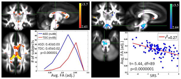
t-statistic maps and distributions of measures for VBM hypotheses in the autism study. The two groups in this study are individuals with autism spectrum disorders (ASD) and typically developing controls (TDC). Left: The left figure displays a voxelwise t-statistic map for group effect in the autism study, thresholded at a significance of p < 0.005 (uncorrected). The insert displays the distributions of mean FA in the cluster in the corpus callosum for the two groups. The figure clearly displays that the mean FA (adjusted for confounds) in the ASD group is shifted to the left, which indicates a decrease in FA relative to the TDC group. Right: The right figure displays a similar map for measuring the effect of SRS on FA in the ASD group. We observe that the average FA (adjusted for confounds) of a cluster in the cerebellum decreases as SRS increases. Not surprisingly, ASD individuals tend to have higher SRS than TDC individuals. The insert demonstrates that, even within the ASD group, higher SRS is associated with a decrease in FA.
Fig. 3.
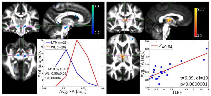
t-statistic maps and distributions of measures for VBM hypotheses in the meditation study with long-term meditators (LTM) and meditation näive practitioners (MNP) as the two groups. Left: The SPM for group effect thresholded at a significance of p < 0.005 (uncorrected). The insert shows that the distributions of mean FA in the cluster in the inferior part of cortico-spinal tract for the two groups. The LTM group mean FA is shifted to the left indicating a decrease in FA. Right: The effect of TLPH on FA in the LTM group. We can observe a positive correlation between the average FA in the cluster (adjusted for confounds) and TLPH.
In the following, we show the results of MVPA for both classification and regression in both the studies. First, we present the test-set bounds or binomial confidence intervals (Kääriäinen and Langford, 2005) for the prediction performance of the linear SVM classifier in Table 4. We then show the classifier and regression performance across the 100 iterations of 10-fold cross-validation in Fig. 4, as distributions of the test-set prediction accuracies of the binary group labels and mean squared errors of prognosis prediction.
Fig. 4.

Distributions of the model-performance metrics for the MVPA hypotheses. We can observe that there is more variance in predicting the group labels in the meditation study compared to the autism study. This is expected because the dichotomy of LTM vs. MNP may not be as strong as those of psychiatric conditions such as ASD vs. TDC. The mean squared error performance also has higher variance in the meditation study.
For classifier models, we show the receiver operating characteristic (ROC) curves. ROC curves plot false positive rate (FPR) vs. true positive rate (TPR) as shown in Figs. 5 and 6. Typically only the area under the curve (AUC) is reported, and the closer it is to 1 the better is the performance of a classifier. However, it is important to understand the various operating regions in the ROC curve, which determine a trade-off between FPR and TPR. To define an operating region, we need user-defined costs for the confusion matrix as shown in Table 5.
Fig. 5.

ROC curve for classification in the autism study. The figure includes confidence intervals for TPR at three different optimal points. As expected, the confidence intervals for TPR become tighter as FPR increases.
Fig. 6.

ROC curve for classification in the meditation study. The figure includes confidence intervals for TPR at three different optimal points. We can observe that at the optimal point with lower FPR, the TPR is much lower compared to that in the autism study again suggesting more difficulty in classifying LTM from MNP than classifying ASD from TDC.
Table 5.
The user-defined costs of making mistakes (similar in spirit to Type I and Type II errors), allow one to identify an optimal operating region on the ROC curve of a classifier.
| True Positive | True Negative | |
|---|---|---|
|
| ||
| Predicted P | c(P|P) | c(P|N) |
| Predicted N | c(N|P) | c(N|N) |
These user-defined costs allow us to identify optimal regions on the ROC curves by moving a line with slope
| (36) |
from top-left (FPR=0,TPR=1) inward until it meets the ROC curve. In addition to the costs of making mistakes, Eq. (36) also takes into account the imbalance in the training data using the ratio N/P which is the ratio of the total number of trainining examples in the “negative” class to the that in the “positive” class. If these costs can be set a priori they can also potentially be used in choosing the MVPA model itself so that one can obtain a model with appropriate trade-off between TPR and FPR on the ROC curves. The costs chosen a posteriori can also be useful in providing a more detailed assessment of the ROC curves using their curvatures at various points rather than just using a summary feature of the curve like AUC.
Although choosing these costs precisely (either a priori or a posteriori) will require strong knowledge from the domain (and sometimes might even be infeasible), we can observe that the slope m is proportional to the ratio of false-postive cost to the false-negative cost if the training data is well balanced. That is,
| (37) |
if N/P = 1 and c(P|P) = 0, c(N|N) = 0. Hence one can choose the ratios of the costs rather than the individual costs themselves. If the ratio is chosen to be greater than 1, the line is more likely to touch the ROC curve towards stricter (lower) FPR regime. If a particular application demands the cost of a miss (false-negative) to be higher than the cost of a false alarm (false-positive) then the slope would be smaller than 1 and the optimal operating region would towards higher FPR regime. The confidence intervals for the corresponding TPR at such optimal points can be computed via any reasonable bootstrapping method. In this paper they are computed using the bias-corrected accelerated (BCa) method (Efron, 1987; Diciccio and Romano, 1988).
For our experiments, we set and define three different optimal points using In our experiments we demonstrate the optimal region calculation (Figs. 5 and 6) using three simple values of m by setting c(N|N) = c(P|P) = 0 and arbitrarily setting c(P|N) as
| (38) |
Hence in this case the c(N|P)s are calculated retrospectively according to Eq. (36). The Table 6 shows the values of c(N|P) for the two different studies.
Table 6.
c (N|P) computed retrospectively using Eq. (36) for the three different settings presented in Eq. (38) and c(P|P) = c(N|N) = 0. One can notice the dependence of the false-negative cost on the imbalance in the training data – with increased N/P ratio the false-negative cost increases with all other factors held constant.
| m, c(P|N) | Autism Study (N/P= 0.5528) | Meditation Study (N/P= 1.0942) |
|---|---|---|
|
| ||
| Setting A | 0.1596 | 0.3159 |
| Setting B | 0.2764 | 0.5471 |
| Setting C | 0.7660 | 1.5162 |
Finally, Figs. 7 (autism study) and 8 (meditation study) show the z-score SPMs to obtain image phenotyping using the MVPA classifiers and regressors. The z-score maps are obtained using average weight vector estimated from the cross-validation folds as described in section 2.2. We can observe that estimated MVPA models in both the studies produce biologically plausible findings. The maps for autism study shown in Fig. 7 also display an interhemispheric asymmetry in significance of the weights, which is consistent with the findings in the autism literature. For example, Lange et al (2010) show that asymmetry is atypical in ASD and serves as a good predictor of the group.
Fig. 7.
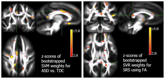
z-score maps thresholded at a significance of p < 0.05 (uncorrected) for MVPA in the autism study. Left: Classification results. Observe that voxels in the cingulum region have significant weight in the classifier model. Right: Regression results of predicting SRS using FA. In both cases, the z-score maps demonstrate that the selected weights are contiguous; we emphasize that this is achieved without using an explicit spatial prior. This result suggests that the estimated MVPA models produce biologically plausible phenotyping information which also shows interhemispheric asymmetry in the importance of the voxels.
4 Discussion and Future Directions
In this paper we presented a unifying treatment of the two major families of neuroimage analyses, namely, the standard voxelwise analysis (VBM) and the emerging multi-voxel pattern analysis (MVPA). Penalized likelihood modeling provides us a natural way to view the models estimated in both families as different combinations of loss and penalty. Hence we call this unified framework as penalized likelihood phenotyping. Although it is increasingly well known that VBM involves estimating a massive number of univariate models and MVPA estimates one massive multivariate model, the proposed unification naturally allows us to identify two, practically relevant, levels of risk assessment of the models in both the families. Such an assessment provides insight into some of the fundamental commonalities and differences between VBM and MVPA and also the challenges in the latter. The first level is concerned with explanatory or predictive power of the models, while the second level of risk arises due to the need for interpretations of the model parameters (MVPA) or collections of models (VBM). In both cases essentially this involves computing tail bounds of various probability distributions or deviation bounds essentially relying on Chernoff type inequalities (Chernoff, 1952).
The first level of risk of the VBM models at individual voxels can be analyzed in a relatively straightforward manner using parametric (such as t or F) or non-parametric distributions (using Monte-Carlo simulations). But for interpreting these models at the neuroanatomical level one needs to analyze the joint risk of all the models to obtain phenotypical information of important regions in the brain. This second level of risk assessment is more complicated and, in fact, this problem, in the general statistical framework of multiple comparisons or familywise error rate, still represents a fertile area of open research in the statistics community. There is no optimal method for solving these problems and the “best” solution is typically a choice from Bonferroni/Sídak type corrections, cluster-based corrections (sometimes invoking results from random field theory) or controlling false discovery rates, depending on the specific instance of the VBM.
In MVPA only one model is estimated; however, it is a large multivariate model (the dimension is on the order of 50,000). Therefore, although MVPA avoids the multiple comparisons problem in the second level, the first level of risk assessment is considerably more challenging. By drawing the fundamental differences between the use of MVPA in artificial intelligence applications versus neuroimaging studies, we demonstrated the need for using metrics beyond the traditional cross-validation accuracies and ROC curves for assessing the risk in prediction power of the models. When using MVPA to extract image based phenotyping information, for interpretation of the brain regions, one still is susceptible to a “multiple comparisons-type” problem since one has to test the significance of each parameter of the massive model. In fact, this is studied in statistics and machine learning as the variable selection problem, which is particularly challenging in the high dimensional low sample size setting (Hesterberg et al, 2008).
For the first level analysis in MVPA, we presented prediction error bounds for the linear SVM classifier models that give us more precise sense of risk in the prediction power of the classifiers. Rather than reporting the usual sample mean and variance of the empirical prediction error rates, which assumes normality of their distribution, we reported precise binomial confidence intervals using a test-set bound. Although normal and binomial distributions behave similarly when the error rates are high, the approximation is not accurate for lower error rates. We also showed how one can define optimal operating regions on the ROC curves using user-defined costs of mistakes/errors and compute confidence intervals on the true detection rates at those regions. We note that the importance of reporting confidence intervals, in addition to test-statistics such as p-values, has also been highlighted elsewhere in cognitive science field (Cohen, 1994). For interpretation of the classifier and regression MVPA models we described a principled way to produce z-statistic maps using z-scores that reflect the relative significance of the parameters in the estimated models. Such a technique also lets us to include non-imaging parameters in the models, thus allowing us to maximize the use of available training data in learning (model estimation).
In this paper we mainly evaluated linear models both for VBM and MVPA which have an advantage in terms of interpretability. One can develop non-parametric as well as implicit non-linear models via kernel methods both for VBM and MVPA(Scholkopf and Smola, 2001; Jäkel et al, 2009; Arthur et al, 2012). Reporting first level risk in these types of models would be similar to the case of linear models. But the interpretation risk analysis becomes harder since, besides having additional estimation challenges, we do not explicitly have access to the parameters of the model. Furthermore, the primary focus of the paper has been on model evaluation via risk assessment and not in obtaining better classification accuracies by using sophisticated feature selection or advanced tensor norm based classifiers. We still would like to note that feature selection can be very useful in neuroimaging since the parameter selection of the model would be based on domain specific knowledge. Such efforts not only can improve the performance in prediction (Chu et al, 2012) but also reduce the risk of false interpretations once the model is trained.
Importance of modeling (including machine learning models) and their careful evaluation has also been highlighted in cognitive science (Shiffrin et al, 2008; Shiffrin, 2010). Computational modeling is not only expanding in neuroimaging but also being embraced in behavioral phenotyping of psychiatric illness (Montague et al, 2012). Hence it becomes important to be cognizant of the model evaluation frameworks and the limits of validatory conclusions one obtains when using MVPA models in neuroscience. In the spirit of understanding the relevance and importance of MVPA in neuroscience, there has also been increasing demand on the empirical validation of MVPA models across studies resulting in upcoming packages like PyMVPA (Hanke et al, 2009b,c) which can facilitate neuroimaging researchers to perform cross-center analyses. To the best of our knowledge, this paper is the first to bring the theoretical prediction risk bounds into practice in neuroimaging settings. Our original contribution is in that this is the first work that addresses the problem of risk assessment and image phenotyping in a principled way when applying MVPA for neuroimaging based neuroscience applications by jointly studying VBM and MVPA.
There are several potential avenues of future research along the lines presented in this paper. (1) The test set bounds provide useful information about the prediction error rates of the MVPA classifier models, however they are not tuned for specific models like support vector machines (used in this paper), decision trees and various other variants. We presented a training set based framework for obtaining bounds for specific families of models. But the main challenge is in coming up with clever de-randomization techniques. This is needed so that confidence intervals can be applicable for the specific learned model rather than the family of the learned model. Although there are some techniques such as using unlabeled training data for de-randomization (Kääriäinen and Langford, 2005), incorporating domain specific information from neuroscience and neuroimaging to improve the existing error bounds would be a great direction to pursue. (2) Additionally, computing these error-bounds in a cross-validation setting by taking into account issues like algorithmic stability is of potential interest (Kearns and Ron, 1999). Currently there are no practically applicable results in that direction. (3) Finally, instead of focusing on designing complex MVPA models (i.e. different loss-penalty combinations and non-parametric forms) which could be harder to visualize and interpret, one could focus on sample complexity (Sivan et al, 2012) results for simple linear models and develop experimental design techniques of new studies for achieving computational learnability. This would result in an MVPA analog for power-analyses used for VBM in neuroimaging (Mumford and Nichols, 2008). Such perspectives and techniques introduced in this paper will hopefully allow neuroscientists and neuroimage researchers to use computational modeling to address increasingly sophisticated questions about the brain-behavior relationships in a powerful and rigorous way.
Fig. 8.
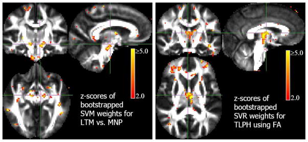
z-score maps thresholded at a significance of p < 0.05 (uncorrected) for MVPA in the meditation study. Left: Classification results. We note that voxels in similar regions as identified by SPMs in VBM (Fig. 3) are found to have significant weights in the classifier model as well. Right: Regression results for predicting TLPH. The z-score maps show that the weights are selected are again contiguous as in Fig. 7 reflecting biological plausibility. We observe bi-lateral significance in both the VBM (Fig. 3) and MVPA phenotyping; this is contrasted with the asymmetry observed in the autism study.
Acknowledgments
We are thankful to Kristen Zygmunt and P. Thomas Fletcher at the University of Utah, for data organization and eddy correction of the diffusion tensor imaging data of the autism study. We also thank Molly DuBray Prigge and Alyson Froehlich for providing us with the subject demographic and assessment information for the autism study. We are extremely thankful to Brianna Schuyller, Amelia Cayo and David Bachubber at the University of Wisconsin-Madison, for assisting us with the sample characteristics of the meditation study.
This work was supported by the NIMH R01 MH080826 (JEL) and R01 MH084795 (JEL) (University of Utah), the NIH Mental Retardation/Developmental Disabilities Research Center (MRDDRC Waisman Center), NIMH 62015 (ALA), the Autism Society of Southwestern Wisconsin, the NCCAM P01 AT004952-04 (RJD and AL) and the Waisman Core grant P30 HD003352-45 (RJD). The content is solely the responsibility of the authors and does not necessarily represent the official views of the National Institutes of Mental Health, the National Institutes of Health or the Waisman Center.
Appendix
For completeness and contrasting with the test-set bounds we derive the training-set bounds for support vector machines (SVMs) in this appendix. First, we need to define a special notion of deviation between ε̂ and ε for analytical reasons. The following provides a notion of “KL-divergence” between two variables p, q ∈ [0, 1],
| (39) |
When , the Chernoff bound (Chernoff, 1952) relates Eq. (39) and the binomial tail (25) as
| (40) |
Now if we restrict the tail probability to α then we have
| (41) |
The above inequality implies (Langford and Shawe-taylor, 2002),
| (42) |
This can be interpreted as the chance that the “deviation” between ε̂ and ε is greater than is less than α.
This bound is also a test-set bound. Although it is looser than Eqs. (26) and (29) it has an analytic form since we approximate FBin by Eq. (40). This analytic test-set bound can then be modified into a practical training-set bounds known as PAC-Bayesian bounds, since these bounds are based on the “priors” on the class of MVPA models.
We need to define two quantities (1) the “prior” (
 ) on the MVPA models in the class being considered (here SVMs). The prior can capture descriptive complexity of the models. (2) The second quantity called “posterior” (
 ) of the estimated/trained/learnt MVPA model that can capture the stability in the estimated parameters of the model. For SVMs we can use
| (43) |
which is an isotropic multivariate Gaussian distribution in p − 1 dimensions (since we exclude the bias in these derivations). The posterior distribution could be defined as
| (44) |
The PAC-Bayes risk assessment depends on the following two expected/stochastic error rates
| (45) |
| (46) |
With these quantities at hand Langford and Shawe-taylor (2002) show the following bound
| (47) |
This bound can be interpreted as, the chance of divergence/deviation between expected empirical error rate and expected true error rate (of a given class of MVPA models - SVMs here) being large can be constrained. Notice the key difference between the above PAC-Bayes bound and Eq. (42). In the case of PAC-Bayes we are assessing risk in terms of the expected error rates rather than the observed error rates. Further the bound says there exists an MVPA model that satisfies the inequality and is dependent on the posterior
. Depending on the concentration/peakiness of
this can be used to reflect the risk of the specific model estimated. We can note that the bound on deviation is dependent on μ in addition to the user-set α. In practice a search needs to be performed for μ in some range to find the tightest possible bound. Thus we can observe that although training-set bounds can be specifically derived and computed for a particular class of MVPA models, there is a trade-off in practice by a need to set additional tuning parameters.
Footnotes
These are also known as voxel based analyses (VBA) or voxel based morphometry (VBM). Also there are popular, mathematically equivalent, variants of VBM such as region-of-interest (ROI) analysis (Nieto-Castanon et al, 2003).
As is standard in the statistics literature we use the acronym GLM for generalized linear model, not general linear model. We broadly use the term linear model (LM) to include what some authors might call the general linear model. The key point is that the LM is a special case of GLM and assumes the error distribution is normally distributed whereas the error distribution in GLM can belong to the more general exponential dispersion family.
Whether MVPA denotes multi-variate pattern analysis or multi-voxel pattern analysis, it has the same meaning (Carp et al, 2011).
We also note that in both VBM and MVPA, Y can also belong to ℝn×k for k > 1 but we shall not consider that class of models in this manuscript.
The tensors in this case are 3rd order, i.e. their elements are indexed by three numbers, while a diffusion tensor (introduced in Section 2.3) is of 2nd order and can be treated as a regular matrix.
We will observe similar statements arising in level 1 risk assessment of the MVPA models where the voxels are treated jointly.
MVPA are quite prevalent and span applications beyond just those based on imaging data.
Compare this with the typical p-values in VBM that allow us to control the first level risk under 0.05 and the multiple comparisons potentially resulting in similar practically un-useful statements.
Humans can quickly (in one pass) isolate wrong findings such as misclassification of cats as dogs.
As a comparison, imagine a setting in which one is given an estimated mean which is expected to follow a student-t distribution, but is not given the degrees of freedom to know which t-distribution to be used for computing the tail-probability.
Camino is an open-source Diffusion-MRI processing software library.
Contributor Information
Nagesh Adluru, Email: adluru@wisc.edu, University of Wisconsin-Madison.
Bret M. Hanlon, University of Wisconsin-Madison
Antoine Lutz, University of Wisconsin-Madison.
Janet E. Lainhart, University of Utah
Andrew L. Alexander, University of Wisconsin-Madison
Richard J. Davidson, University of Wisconsin-Madison
References
- Adluru N, Hinrichs C, Chung M, Lee J, Singh V, Bigler E, Lange N, Lainhart J, Alexander A. IEEE Engineering in Medicine and Biology Society. 2009. Classification in DTI using shapes of white matter tracts; pp. 2719–2722. [DOI] [PMC free article] [PubMed] [Google Scholar]
- Adluru N, Ennis C, Davidson R, Alexander A. Max margin general linear modeling for neuroimage analysis. IEEE Workshop on Mathematical Modeling in Biomedical Image Analysis; 2012. pp. 105–110. [DOI] [PMC free article] [PubMed] [Google Scholar]
- Alexander A, Lee J, Lazar M, Field A. Diffusion tensor imaging of the brain. Neurotherapeutics. 2007;4:316–329. doi: 10.1016/j.nurt.2007.05.011. [DOI] [PMC free article] [PubMed] [Google Scholar]
- Anderson M, Oates T. A critique of multi-voxel pattern analysis. In: Ohlsson S, Catrambone R, editors. Proceedings of the 32nd Annual Meeting of the Cognitive Science Society. 2010. pp. 1511–16. [Google Scholar]
- Arthur G, Karsten MB, Malte JR, Bernhard S, Alexander JS. A kernel two-sample test. Journal of Machine Learning Research. 2012;13:723–773. [Google Scholar]
- Basser P, Pierpaoli C. Microstructural and physiological features of tissues elucidated by quantitative-diffusion-tensor MRI. J Magn Reson. 1996;111:209–219. doi: 10.1006/jmrb.1996.0086. [DOI] [PubMed] [Google Scholar]
- Basser P, Mattiello J, Bihan D. Estimation of the effective self -diffusion tensor from NMR spin echo. J Magn Reson. 1994;103:247–254. doi: 10.1006/jmrb.1994.1037. [DOI] [PubMed] [Google Scholar]
- Batmanghelich N, Dong A, Taskar B, Davatzikos C. Regularized tensor factorization for multi-modality medical image classification. Med Image Comput Comput Assist Interv. 2011;14:17–24. doi: 10.1007/978-3-642-23626-6_3. [DOI] [PubMed] [Google Scholar]
- Beckmann C, Smith S. Tensorial extensions of independent component analysis for multisubject fMRI analysis. NeuroImage. 2005;25:294–311. doi: 10.1016/j.neuroimage.2004.10.043. [DOI] [PubMed] [Google Scholar]
- Benjamini Y, Hochberg Y. Controlling the false discovery rate: a practical and powerful approach to multiple testing. Journal of the Royal Statistical Society. 1995;57(1):125–133. [Google Scholar]
- Bickel P, Li B, Tsybakov A, van de Geer S, Yu B, Valdés T, Rivero C, Fan J, van der Vaart A. Regularization in statistics. Test. 2006;15(2):271–344. [Google Scholar]
- Bunea F, She Y, Ombao H, Gongvatana A, Devlin K, Cohen R. Penalized least squares regression methods and applications to neuroimaging. Neuroimage. 2011;55(4):1519–1527. doi: 10.1016/j.neuroimage.2010.12.028. [DOI] [PMC free article] [PubMed] [Google Scholar]
- Carp J, Park J, Polk T, Park D. Age differences in neural distinctiveness revealed by multi-voxel pattern analysis. Neuroimage. 2011;56(2):736–743. doi: 10.1016/j.neuroimage.2010.04.267. [DOI] [PMC free article] [PubMed] [Google Scholar]
- Carroll M, Cecchi G, Rish I, Garg R, Rao A. Prediction and interpretation of distributed neural activity with sparse models. Neuroimage. 2009;44:112–122. doi: 10.1016/j.neuroimage.2008.08.020. [DOI] [PubMed] [Google Scholar]
- Chang C, Lin C. LIBSVM: a library for support vector machines. 2001 Software available at http://www.csie.ntu.edu.tw/~cjlin/libsvm.
- Chernoff H. A measure of asymptotic efficiency of tests of a hypothesis based upon the sum of the observations. Annals of Mathematical Statistics. 1952;24:493–507. [Google Scholar]
- Cho Y, Seong J, Jeong Y, Shin S ADNI . Individual subject classification for alzheimer’s disease based on incremental learning using a spatial frequency representation of cortical thickness data. Neuroimage. 2012;59(3):2217–2230. doi: 10.1016/j.neuroimage.2011.09.085. [DOI] [PMC free article] [PubMed] [Google Scholar]
- Chu C, Hsu A, Chou K, Bandettini P, Lin C ADNI . Does feature selection improve classification accuracy? impact of sample size and feature selection on classification using anatomical magnetic resonance images. Neuroimage. 2012;60(1):59–70. doi: 10.1016/j.neuroimage.2011.11.066. [DOI] [PubMed] [Google Scholar]
- Cohen J. The earth is round (p < .05) American Psychologist. 1994:997–1003. [Google Scholar]
- Constantino J, Przybeck T, Friesen D, Todd R. Reciprocal social behavior in children with and without pervasive developmental disorders. Journal of Developmental and Behavioral Pediatrics. 2000;21:2–11. doi: 10.1097/00004703-200002000-00002. [DOI] [PubMed] [Google Scholar]
- Diciccio T, Romano J. A review of bootstrap confidence intervals. Journal of the Royal Statistical Society Series B (Methodological) 1988;50(3):338–354. [Google Scholar]
- Efron B. Better bootstrap confidence intervals. Journal of American Statistics Association. 1987;82:171–185. doi: 10.1080/10618600.2020.1714633. [DOI] [PMC free article] [PubMed] [Google Scholar]
- Fraley C, Hesterberg T. Least angle regression and lasso for large datasets. Statistical Analysis and Data Mining. 2009;1(4):251–259. [Google Scholar]
- Friedman J, Hastie T, Tibshirani R. Regularization paths for generalized linear models via coordinate descent. Journal of Statistical Software. 2010;33(1):1–22. [PMC free article] [PubMed] [Google Scholar]
- Halchenko Y, Hanke M. Advancing neuroimaging research with predictive multivariate pattern analysis. 2010. [Google Scholar]
- Hanke M, Halchenko Y, Sederberg P, Hanson S, Haxby J, Pollmann S. Pymvpa: A python toolbox for multivariate pattern analysis of fmri data. Neuroinformatics. 2009a;7(1):37–53. doi: 10.1007/s12021-008-9041-y. [DOI] [PMC free article] [PubMed] [Google Scholar]
- Hanke M, Halchenko Y, Sederberg P, Hanson S, Haxby J, Pollmann S. PyMVPA: A python toolbox for multivariate pattern analysis of fMRI data. Neuroinformatics. 2009b;7:37–53. doi: 10.1007/s12021-008-9041-y. [DOI] [PMC free article] [PubMed] [Google Scholar]
- Hanke M, Halchenko YO, Sederberg PB, Olivetti E, Fründ I, Rieger JW, Herrmann CS, Haxby JV, Hanson SJ, Pollmann S. PyMVPA: a unifying approach to the analysis of neuroscientific data. Frontiers in Neuroinformatics. 2009c;3(3) doi: 10.3389/neuro.11.003.2009. [DOI] [PMC free article] [PubMed] [Google Scholar]
- Hastie T, Tibshirani R, Friedman J. The Elements of Statistical Learning. 2. Springer; 2009. [Google Scholar]
- Hesterberg T, Choi N, Meier L, Fraley C. Least angle and ℓ1 penalized regression: A review. Statistics Surveys. 2008;2:61–93. [Google Scholar]
- Hinrichs C, Singh V, Mukherjee L, Xu G, Chung M, Johnson S ADNI . Spatially augmented LP-boosting for AD classification with evaluations on the ADNI dataset. Neuroimage. 2009;48(1):138–149. doi: 10.1016/j.neuroimage.2009.05.056. [DOI] [PMC free article] [PubMed] [Google Scholar]
- Hinrichs C, Singh V, Xu G, Johnson S ADNI . Predictive markers for AD in a multi-modality framework: an analysis of MCI progression in the ADNI population. Neuroimage. 2011;55(2):574–589. doi: 10.1016/j.neuroimage.2010.10.081. [DOI] [PMC free article] [PubMed] [Google Scholar]
- Huber P. Robust Statistics. John Wiley and Sons; New York: 1981. [Google Scholar]
- Ingalhalikar M, Parker D, Bloy L, Roberts T, Verma R. Diffusion based abnormality markers of pathology: Toward learned diagnostic prediction of ASD. NeuroImage. 2011:918–927. doi: 10.1016/j.neuroimage.2011.05.023. [DOI] [PMC free article] [PubMed] [Google Scholar]
- Jäkel F, Schlkopf B, Wichmann F. Does cognitive science need kernels? Trends in Cognitive Sciences. 2009;13:381–388. doi: 10.1016/j.tics.2009.06.002. [DOI] [PubMed] [Google Scholar]
- Jones D, Simmons A, Williams S, Horsfield M. Non-invasive assessment of axonal fiber connectivity in the human brain via diffusion tensor mri. Magn Reson Med. 1999;42:37–41. doi: 10.1002/(sici)1522-2594(199907)42:1<37::aid-mrm7>3.0.co;2-o. [DOI] [PubMed] [Google Scholar]
- Kääriäinen M, Langford J. A comparison of tight generalization error bounds. International conference on Machine learning; 2005. pp. 409–416. [Google Scholar]
- Kanungo T, Haralick R. Tech rep. University of Washington; 1995. Multivariate hypothesis testing for gaussian data: Theory and software. [Google Scholar]
- Kearns M, Ron D. Algorithmic stability and sanity-check bounds for leave-one-out cross-validation. Neural Computation. 1999;11:1427–1453. doi: 10.1162/089976699300016304. [DOI] [PubMed] [Google Scholar]
- Kolda TG, Bader BW. Tensor decompositions and applications. SIAM Review. 2009;51(3):455–500. [Google Scholar]
- Kotsia I, Guob W, Patrasa I. Higher rank support tensor machines for visual recognition. Pattern Recognition. 2012;45(12):4192–4203. [Google Scholar]
- Lange N, Dubray M, Lee J, Froimowitz M, Froehlich A, Adluru N, Wright B, Ravichandran C, Fletcher P, Bigler E, Alexander A, Lainhart J. Atypical diffusion tensor hemispheric asymmetry in autism. Autism Research. 2010:350–358. doi: 10.1002/aur.162. [DOI] [PMC free article] [PubMed] [Google Scholar]
- Langford J, Shawe-taylor J. PAC-Bayes & margins. Advances in Neural Information Processing Systems. 2002:439–446. [Google Scholar]
- Le Bihan D, Mangin J, Poupon C, Clark C, Pappata S, Molko N, HC Diffusion tensor imaging: concepts and applications. Journal of Magnetic Resonance Imaging. 2001;13(4):534–546. doi: 10.1002/jmri.1076. [DOI] [PubMed] [Google Scholar]
- Liu M, Zhang D, Shen D ADNI . Ensemble sparse classification of Alzheimer’s disease. NeuroImage. 2012;60:1106–1116. doi: 10.1016/j.neuroimage.2012.01.055. [DOI] [PMC free article] [PubMed] [Google Scholar]
- Marquardt D, Snee R. Ridge regression in practice. The American Statistician. 1975;29(1):3–20. [Google Scholar]
- McCullagh P, Nelder J. Generalized linear models. Chapman & Hall/CRC; 1989. [Google Scholar]
- Mitchell T. From journal articles to computational models: a new automated tool. Nature Methods. 2011;8(8):627–628. doi: 10.1038/nmeth.1661. [DOI] [PubMed] [Google Scholar]
- Montague P, Dolan R, Friston K, Dayan P. Computational psychiatry. Cell Special Issue: Cognition in Neuropsychiatric Disorders. 2012;16(1):72–80. doi: 10.1016/j.tics.2011.11.018. [DOI] [PMC free article] [PubMed] [Google Scholar]
- Mori S, Kaufmann W, Davatzikos C, Stieltjes B, Amodei L, Fredericksen K, Pearlson G, Melhem E, Solaiyappan M, Raymond G, Moser H, van Zijl P. Imaging cortical association tracts in the human brain using diffusion-tensor-based axonal tracking. Magn Reson Med. 2002;47:215–223. doi: 10.1002/mrm.10074. [DOI] [PubMed] [Google Scholar]
- Mumford J, Nichols T. Power calculation for group fmri studies accounting for arbitrary design and temporal autocorrelation. 2008;39(1):261–268. doi: 10.1016/j.neuroimage.2007.07.061. [DOI] [PMC free article] [PubMed] [Google Scholar]
- Nichols T, Holmes A. Nonparametric permutation tests for functional neuroimaging: a primer with examples. Hum Brain Mapp. 2002;15(1):1–25. doi: 10.1002/hbm.1058. [DOI] [PMC free article] [PubMed] [Google Scholar]
- Nieto-Castanon A, Ghosh S, Tourville J, Guenther F. Region of interest based analysis of functional imaging data. Neuroimage. 2003;19(4):1303–1316. doi: 10.1016/s1053-8119(03)00188-5. [DOI] [PubMed] [Google Scholar]
- Norman K, Polyn S, Detre G, Haxby J. Beyond mind-reading: multi-voxel pattern analysis of fMRI data. Trends in cognitive sciences. 2006;10(9):424–430. doi: 10.1016/j.tics.2006.07.005. [DOI] [PubMed] [Google Scholar]
- Pachauri D, Hinrichs C, Chung M, Johnson S, Singh V. Topology-based kernels with application to inference problems in Alzheimer’s disease. IEEE Trans Med Imaging. 2011;30(10):1760–1770. doi: 10.1109/TMI.2011.2147327. [DOI] [PMC free article] [PubMed] [Google Scholar]
- Park M, Hastie T. ℓ1-regularization path algorithm for generalized linear models. Royal Statistical Society Series B Statistical Methodology. 2007;69(4):659. [Google Scholar]
- Pereira F, Mitchell T, Botvinick M. Machine learning classifiers and fMRI: a tutorial overview. Neuroimage. 2009;45(1):S199–S209. doi: 10.1016/j.neuroimage.2008.11.007. [DOI] [PMC free article] [PubMed] [Google Scholar]
- Ryali S, Supekar K, Abrams D, Menon V. Sparse logistic regression for whole-brain classification of fMRI data. Neuroimage. 2010;18:752–764. doi: 10.1016/j.neuroimage.2010.02.040. [DOI] [PMC free article] [PubMed] [Google Scholar]
- Scholkopf B, Smola A. Learning with Kernels: Support Vector Machines, Regularization. MIT Press; Cambridge, MA: 2001. [Google Scholar]
- Shi Z, Zheng T, Han J. Trace Norm Regularized Tensor Classification and Its Online Learning Approaches. 2011. ArXiv e-prints 1109.1342. [Google Scholar]
- Shiffrin R. Perspectives on modeling in cognitive science. Topics in Cognitive Science. 2010;2(4):736–750. doi: 10.1111/j.1756-8765.2010.01092.x. [DOI] [PubMed] [Google Scholar]
- Shiffrin R, Lee M, Kim W, Wagenmakers E. A survey of model evaluation approaches with a tutorial on hierarchical bayesian methods. Cognitive Science. 2008;32:1248–1284. doi: 10.1080/03640210802414826. [DOI] [PubMed] [Google Scholar]
- Signoretto M, De Lathauwer L, Suykens J. Tech rep. K.U. Leuven; 2011. Nuclear norms for tensors and their use for convex multilinear estimation. [Google Scholar]
- Sivan S, Nati S, Naftali T. Characterizing the sample complexity of large-margin learning with second-order statistics. CoRR. 2012:1204–1276. [Google Scholar]
- Smith S, Nichols T. Threshold-free cluster enhancement: addressing problems of smoothing, threshold dependence and localisation in cluster inference. Neuroimage. 2009;44(1):83–98. doi: 10.1016/j.neuroimage.2008.03.061. [DOI] [PubMed] [Google Scholar]
- Smith S, Jenkinson M, Woolrich M, Beckmann C, Behrens T, Johansen-Berg H, Bannister P, De Luca M, Drobnjak I, Flitney D, Niazy R, Saunders J, Vickers J, Zhang Y, De Stefano N, Brady J, Matthews P. Advances in functional and structural MR image analysis and implementation as FSL. NeuroImage. 2004;23:208–219. doi: 10.1016/j.neuroimage.2004.07.051. [DOI] [PubMed] [Google Scholar]
- Taylor J, Worsley K. Random fields of multivariate test statistics, with applications to shape analysis. Annals of Statistics. 2008;36:1–27. [Google Scholar]
- Tibshirani R. Regression shrinkage and selection via the lasso. Journal of the Royal Statistical Society Series B (Methodological) 1996:267–288. [Google Scholar]
- Valiant L. A theory of the learnable. Commun ACM. 1984;27(11):1134–1142. [Google Scholar]
- Vapnik V, Chervonenkis A. On the uniform convergence of relative frequencies of events to their probabilities. Theory of Probability and its Applications. 1971;16(2):264–280. [Google Scholar]
- Vounou M, Nichols T, Montana G ADNI . Discovering genetic associations with high-dimensional neuroimaging phenotypes: a sparse reduced-rank regression approach. Neuroimage. 2010;53:114–1159. doi: 10.1016/j.neuroimage.2010.07.002. [DOI] [PMC free article] [PubMed] [Google Scholar]
- Wolf L, Jhuang H, Hazan T. Modeling appearances with low-rank SVM. Computer Vision and Pattern Recognition. 2007:1–6. [Google Scholar]
- Worsley K, Marrett S, Neelin P, Vandal A, Friston K, Evans A. A unified statistical approach for determining significant signals in images of cerebral activation. Hum Brain Mapp. 1996;4:58–73. doi: 10.1002/(SICI)1097-0193(1996)4:1<58::AID-HBM4>3.0.CO;2-O. [DOI] [PubMed] [Google Scholar]
- Worsley K, Taylor J, Tomaiuolo F, Lerch J. Unified univariate and multivariate random field theory. Neuroimage. 2004;23:189–195. doi: 10.1016/j.neuroimage.2004.07.026. [DOI] [PubMed] [Google Scholar]
- Worsley K, Taylor J, Carbonell F, Chung M, Duerden E, Bernhardt B, Lyttelton O, Boucher M, Evans A. SurfStat: A Matlab toolbox for the statistical analysis of univariate and multivariate surface and volumetric data using linear mixed effects models and random field theory. Neuroimage. 2009;47:S102–S102. [Google Scholar]
- Yarkoni T, Poldrack R, Nichols T, Van Essen D, Wager T. Large-scale automated synthesis of human functional neuroimaging data. Nature Methods. 2011;8(8):665–670. doi: 10.1038/nmeth.1635. [DOI] [PMC free article] [PubMed] [Google Scholar]
- Yuan G, Ho C, Lin C. Tech rep. National Taiwan University; 2011. An improved GLMNET for ℓ1-regularized logistic regression and support vector machines. [Google Scholar]
- Zhang D, Shen D ADNI . Multi-modal multi-task learning for joint prediction of multiple regression and classification variables in Alzheimer’s disease. Neuroimage. 2012;59(2):895–907. doi: 10.1016/j.neuroimage.2011.09.069. [DOI] [PMC free article] [PubMed] [Google Scholar]
- Zhang H, Yushkevich P, Alexander D, Gee J. Deformable registration of diffusion tensor MR images with explicit orientation optimization. Medical Image Analysis. 2006;10:764–785. doi: 10.1016/j.media.2006.06.004. [DOI] [PubMed] [Google Scholar]