The Impact of Childhood Health on Adult Labor Market Outcomes

Abstract

This paper examines impacts of childhood health on SES outcomes observed during adulthood—levels and trajectories of education, family income, household wealth, individual earnings and labor supply. The analysis is conducted using data that collects these SES measures in a panel who were originally children and who are now well into their adult years. Since all siblings are in the panel, one can control for unmeasured family and neighborhood background effects. With the exception of education, poor childhood health has a quantitatively large effect on all these outcomes. Moreover, these estimated effects are larger when unobserved family effects are controlled. (JEL codes; I₁₀, J₀₀)

There is renewed scholarly and policy interest in why adults of lower socio-economic status (SES) have worse health outcomes. No matter which measures of SES are used (income, wealth, or education), the evidence that this association is large is abundant (Marmot, 1999; Smith, 1999). A key issue concerns the extent to which childhood health status affects levels and trajectories of the most central measures of SES including education, income, and wealth during one’s adult years. But estimating this relationship is difficult, as it requires data that follow individuals from their childhood years into a significant part of their adulthood, all the while simultaneously measuring health and these key SES concepts. Since unmeasured attributes of the family, neighborhood and environment in which people are raised may be determinants of their adult outcomes and trajectories, data must permit some control for them, especially that undoubtedly large sub-component that is unmeasured in most surveys.

This paper uses unique data derived from the Panel Survey of Income Dynamics (PSID) that has followed groups of siblings and their parents for as long as 30 years. Throughout that period, information on education, income, wealth, and health were collected prospectively on all parties. Following siblings from the same family offers an excellent opportunity to control for unmeasured family and other background effects common to children raised in the same family especially in light of the detailed and long histories of economic status available for these children when they are adults in the PSID. Using this data, I present estimates that indicate that health conditions during childhood have quantitatively large impacts on virtually all key adult indicators of socioeconomic status used by economists.

This paper is divided into three sections. The first briefly summarizes some recent contributions by economists on the question of the origins and impact of childhood health on adult outcomes. Section 2 highlights the salient strengths and weaknesses of the data that will be used in the analysis. The final section contains empirical models that investigate the impact of family background and childhood attributes on later life health and several central SES outcomes and trajectories. In particular, these analyses will focus on the question of the impact of childhood health on later adult outcomes, including completed levels of schooling and household and individual income and earnings, and household wealth.

I. Background

The revival of interest in determinants and consequences of poor childhood health can be traced partly to the impact of studies by David J. Barker and his associates (1997). They provide evidence that even nutrition in utero impacts health outcomes much later during one’s adulthood. Some of this research is derived from animal studies where purposely-deprived fetal growth was shown to affect subsequent mortality. While controversial, data from natural experiments lend some support to this view. For example, Ravelli et al. (1998) studied people born in Amsterdam who were exposed pre-natally to famine conditions in 1944–1945. When compared to those conceived a year before or after the famine, prenatal exposure to famine, especially during late gestation, was linked to decreased glucose tolerance in adults producing higher risks of diabetes.

In the last few years, economists have done some insightful work on this topic. Using data from two health surveys (NHANES III and the National Health Interview Survey) as well as the PSID child development supplement (PSID-CDS), Case, Lubotsky, and Paxson (2002) demonstrated that the relationship between SES and health has it origins in early childhood and expanded as children age. They report a strong relationship between parental income and several salient measures of child health including common childhood chronic health conditions, a relationship that accumulated as children age. This relationship persisted even after controlling for other measured background characteristics, including parental education.

Currie and Stabile (2003) report similar findings They argue that the gradient emerges when people become adults not because lower-SES children have a more difficult time recovering from a health shock but rather that low-SES children receive more frequent health shocks during childhood. They also report that poor childhood health disadvantages children in part to lower cognitive and academic achievement as indicated by higher probabilities of grade repetition and lower math and reading test scores among children in poorer health.

Case, Fertig, and Paxson (2005) investigated persistent impacts of childhood health on adult health, employment, and some measures of SES using a 1958 British birth cohort who were followed prospectively into their adult years. They find that people who experienced poorer health outcomes either in terms of low birth weight or the presence of chronic conditions when they were children not only had worse health as adults, but they passed fewer O-level exams, worked less during their adult years, and had lower occupational status at age 42 even after some standard key measures of parental background such as education and income were controlled for.

Despite the rich set of controls available especially in the prospective British cohort studies, this research cannot rule out the possibility that the role of child health in determining adult SES, are in fact driven by other, unobserved characteristics of the family or home environment that are correlated with child health and unmeasured family background effects. For example, Currie, Shields, and Price (2004) estimate that among a sample of English siblings 1997–2002, as much as 60% of the total variation in child health might be explained by unobserved family effects.¹ Some of the child health effects identified in the papers cited above could be due to similar unobserved heterogeneity in the cohort study data.

Several other studies suggest that childhood health may be important for adult outcomes. For example, using a sample of Norwegian twins, Black, Devereux, and Salvanes (2005) find that low birth weight babies have worse short-run (mortality) and long-run outcomes (schooling and earnings). Within-twin estimates reduced estimated short-run effects but not the longer-run impacts on labor market outcomes. Similarly, Almond, Chay, and Lee (2005) using a sample based on twins suggest that the estimated short-run health costs of low birth weight may be significantly overstated. Finally, Oreopoulos et al. (2006) using a very interesting administrative sample of siblings and twins drawn from administrative records in Canada report that poor infant health is a strong predictor of future education and the take-up and duration on social assistance.

II. Data

The PSID has gathered almost 30 years of extensive economic and demographic data on a nationally representative sample of approximately 5000 (original) families and 35,000 individuals living in those families. Details on family income and its components and labor market activity have been obtained in each wave since the inception of PSID in 1968. Starting in 1984 and in five-year intervals until 1999, PSID asked a set of questions to measure household wealth. Starting in 1997, the PSID switched to a two-year periodicity, and wealth modules are now included as part of the core interview. The PSID is rightly recognized as one of the premier general-purpose panel survey measuring several key dimensions of adult labor market outcomes.

The PSID has collected information on self-reported general health status (the standard five-point scale from excellent to poor) since 1984 and starting in 1999 and for all subsequent waves, information was gathered on the prevalence and incidence of a list of chronic conditions for the respondent and spouse—heart disease, stroke, heart attack, hypertension, cancer, diabetes, chronic lung disease, asthma, arthritis, and emotional, nervous, or psychiatric problems.

The PSID permits a long-term perspective on impacts of childhood health. Since many panel members were in the PSID since 1967, the entire past financial histories can be exploited. This is especially important for children in the original panel or born thereafter. When these children become panel members on their own, we have SES histories yearly for them and their parents. Since the same applies to their siblings, the PSID offers a nice opportunity to model and control for family background effects combined with a much richer history of economic status as an adult than exists in any of the other good current studies on this question.

The PSID has both advantages and disadvantages for studying the impact of childhood health on later life outcomes. There are two main disadvantages. The most obvious is that measures of childhood health conditions are limited and available only for PSID respondents who were adults in the 1999 wave. In particular, one must rely on a single index—a retrospective self-evaluation using the standard five-point scale (excellent, very good, good, fair, or poor) of general state of one’s health when one was less than 17 years old asked in the 1999 wave.² Several studies have pointed to specific aspects of childhood health as being particularly important, including low birth weight or APGAR scores at birth (Oreopoulos et al. (2006)) or specific childhood illnesses (Case, Lubotsky, and Paxson (2002)). A counterpoint to the obvious limitations of using a single health index is that this one attempts to obtain a summary measure of the complete childhood health experience, a useful concept to have in mind.³ Some issues with this retrospective childhood health question are discussed in detail below.

The second disadvantage is that to have the most comprehensive measures of family background one must select children of the original PSID respondents which implies that adult outcomes are necessarily limited to early and mid adulthood. For example, a 16 year old living in the parental home in 1968 would only be approaching age 50 by the critical 1999 wave. If we take age 25 as the minimum cutoff for monitoring adult outcomes, we can only include all children 16 and younger in 1968 and all children subsequently born up to 1974.

Fortunately, the advantages are also unique. The PSID is the best American panel data for the two most important financial SES measures (income and wealth) for a sample spanning the full age distribution. Most important, it offers a rare opportunity to examine generational and family effects. As part of its structure, the PSID follows all family members of the 1967 panel of respondents as well as any new family members who arrive subsequently. Thus any children of the original PSID members as well as their siblings are panel members.

For these PSID panel children and their siblings, the full array of SES and health measures potentially exists each year not only for both themselves and the parental households from which they came but for their siblings when they become independent households. For this sample we have their own and their siblings income histories up to the 1999 wave as well as that of their parents (the original PSID sample members). We would also have for all siblings and parents the type of health data described above for all PSID respondents.

III. The Impacts of Family Background and Childhood Health on Adult SES

This paper rests on three substantive points. First, outcomes observed throughout one’s adult years often are the legacy of events during childhood and health is one of the best examples of that link. Figure 1 provides evidence of this link by plotting contemporaneous self-reports of general health status by age against self-reports about general childhood health status. For both childhood and adult health, good health is a report of excellent or very good and all other categories are labeled poor. Individuals in better health during childhood have adult health levels and trajectories much above those whose childhood health was poor. This association is quantitatively important. At age 25, those in ‘good’ health during their childhood years reported levels of ‘good’ health as an adult 10 percentage points higher than those whose childhood health was ‘poor.’ This disparity grows to more than 25 percentage points by the early 40’s, suggesting that childhood health affects trajectories as well as initial health levels during the adult years.

Fig. 1.

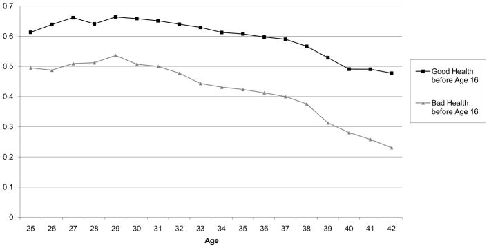
Self-reported Health Status Excellent or Very Goood by Health Status before Age 16

The second and third points are that this link between child and adult health is partly the consequence of many observable and unobservable attributes of childhood family background. The importance of unmeasured family effects is a principal point of this paper and is discussed in detail below. To document this for measured family effects, Table 1 summarizes results from a simple model of generational health transmission through disease prevalence. Besides standard demographic attributes, models include controls for a quadratic in respondent’s age, mother’s and father’s education, and the ln of the average parental income computed during all childhood years available (from birth to age 16 in years present in the PSID panel). Throughout, all financial variables are measured in 2001 dollars. The childhood health variable is a dummy indicating a respondents’ health during childhood up to age 16 was either excellent or very good.

Table 1.

Probits Predicting Adult Disease Prevalence in the 1999 PSID

	Severe Condition		Minor Condition
	Coef.	“t”	Coef.	“t”
Age in 1	−0.005	(0.07)	−0.021	(0.39)
Age in 1999 squared	0.003	(0.36)	0.001	(1.07)
Black	−0.260	(2.20)	0.048	(0.66)
Hispanic	−0.370	(1.61)	−0.103	(0.65)
Female	0.327	(4.38)	0.001	(0.02)
Health up to age16 EX-VG	−0.329	(4.13)	−0.195	(3.02)
Ln parental income ages1–16	−0.168	(2.16)	−0.090	(1.58)
Mother Ed 12–15 years	−0.091	(1.05)	−0.165	(2.44)
Mother Ed college or more	0.012	(0.09)	−0.252	(2.28)
Father Ed 12–15 years	0.131	(1.45)	0.077	(1.14)
Father Ed college or more	0.048	(0.37)	−0.041	(0.42)
A parent has severe health condition	0.141	(1.62)	0.148	(2.26)
A parent has minor health condition	−0.019	(0.21)	0.152	(2.03)
Constant	0.098	(0.07)	−0.252	(0.24)

Note: The sample consists of about 3,053 PSID respondents present during the 1999 PSID wave who were also children of the original PSID respondents. These respondents were at most 16 in 1968 or subsequently born between 1968 and 1984. These models also contain indicator variables for missing information on each parent, mother died and age of her death, father died and age of his death. The first column for each model lists the estimated coefficients from the probits. T statistics in parenthesis are based on robust standard errors.

Since there are not sufficient data to conduct a disease-by-disease analysis, two adult health outcomes are modeled—whether the respondent has a chronic condition rated severe or one rated minor. Severe conditions were defined as cancer, heart condition, stroke, and diseases of the lung. All other onsets (hypertension, arthritis, diabetes) are minor. To isolate inter-generational transmission of disease, two variables are added indicating the at least one parent has a major chronic condition and that at least one parent had a minor chronic condition.⁴ This analysis cannot tell us whether generational health transmissions are due to shared biology or shared environment, as any estimated linkage is some combination of these mechanisms.⁵

Table 1 suggests a key role for family background on adult health. To use one example, higher incomes of parents when one was a child lower the probability of having a chronic condition during adulthood although this is only statistically significant for severe diseases. Similarly whether through biology or common impacts of a shared family environment or shared health behaviors, diseases of parents are associated with those of their adult children. Since ages of the adult PSID children in the sample in Table 1 may still be too young to have many shared severe common conditions with their parents, the transmissions are more transparent for minor chronic conditions. Finally, there is evidence of long legacy health effects spanning from childhood into mid-adulthood. For both minor and severe adult chronic conditions, the odds of having health problems as adults are correlated with general health status in childhood.

A. Estimates on 1999 SES Levels

My primary goal involves estimating impacts of childhood health on several salient adult SES outcomes. This inquiry begins with four key SES outcomes—completed years of schooling, ln family income, household wealth, and individual earnings, all measured in the 1999 PSID when retrospective childhood health was collected. Besides a standard set of demographic controls (age quadratic to capture life-cycle and cohort effects), race (=1 if Black), Hispanic ethnicity (= 1 if Latino), and gender =1 if female)), all models include family background measures of PSID respondents (education of both the mother and father, the average ln parental income during years when the child was less than 17 years old⁶, and the number of siblings).

The sample on which these models are based are PSID respondents present in interview wave 1999 who were no more than 16 years old in 1968 or who were subsequently born into the PSID between the years 1968 and 1974. Results are listed in Table 2 (education), Table 3 (ln family income and household wealth) and Table 4 (individual earnings). Baseline models in each table provide estimates of the magnitude of mean differences across demographic groups, the extended model columns add the set of family background variables, while those in the within sibling columns are fixed effects estimates using differences amongst the siblings of these PSID families. The ‘t’ statistics in parenthesis are based on robust standard errors.

Table 2.

Predicting Levels of Adult Education in the 1999 PSID

	Education in 1999
	Baseline Model		Extended Model		Within Sibling Model
Age in 1999	−0.093	(1.27)	−0.012	(0.19)	−0.134	(1.44)
Age in 1999 squared	0.014	(1.42)	0.001	(0.66)	0.002	(1.55)
Black	−1.178	(14.3)	0.232	(2.57)
Hispanic	−0.412	(1.88)	−0.206	(1.11)
Female	0.100	(1.25)	0.196	(2.92)	0.303	(3.83)
Health up to age 16 EX-VG			0.353	(4.28)	0.114	(1.15)
Ln parental income ages 1–16			0.779	(10.8)	0.363	(1.14)
Mother Ed 12–15 years			0.646	(7.45)
Mother Ed college or more			1.216	(8.97)
Father Ed 12–15 years			0.246	(2.89)
Father Ed college or more			1.406	(11.9)
Number of siblings			−0.127	(6.52)
Constant	14.99	(11.7)	3.429	(2.65)	11.24	(2.92)
N	3069		3055		2248

Note: The sample consists of PSID respondents present during the 1999 PSID wave who were also children of the original PSID respondents. These respondents were at most 16 in 1968 or subsequently born between 1968 and 1984. “t” statistics based on robust standard errors. The within sibling estimates place an additional restriction that there were at least two siblings who were PSID respondents in 1999.

Table 3.

Predicting Adult Ln Household Income and Household Wealth in the 1999 PSID

	Ln Household Income in 1999						Wealth in 1999
	Baseline Model		Extended Model		Within Sibling Model		Extended Model		Within Sibling Model
Age in 1999	0.099	(4.98)	0.093	(4.62)	0.081	(1.80)	1,796	(2.56)	−1,299	(0.31)
Age in 1999 squared	−0.001	(3.93)	−0.001	(3.54)	−0.001	(1.41)	−19.4	(2.00)	44.8	(0.81)
Black	−0.289	(12.1)	−0.083	(2.87)			−2,605	(2.51)
Hispanic	0.021	(0.35)	0.023	(0.40)			19.1	(0.01)
Female	−0.070	(3.26)	−0.057	(2.72)	0.028	(0.73)	1.5	(0.00)	−1,000	(0.28)
Married in 1999	0.664	(28.7)	0.666	(29.5)	0.758	(18.2)	8,589	(10.9)	23,756	(6.24)
Health up to age16 EX-VG			0.130	(5.03)	0.240	(4.98)	1,847	(2.05)	10,005	(2.29)
Ln parental income ages 1–16			0.227	(9.79)	0.011	(0.07)	4,283	(5.18)	11,647	(0.83)
Mother Ed 12–15 years			0.038	(1.37)			325	(0.34)
Mother Ed college or more			0.044	(1.03)			−879	(0.58)
Father Ed 12–15 years			0.060	(2.24)			−1,489	(1.60)
Father Ed college or more			0.030	(0.79)			−1,017	(0.76)
Number of siblings			−0.017	(2.81)			−245.7	(1.15)
Education in 1999	0.123	(23.3)	0.097	(16.7)	0.099	(7.68)	1,652	(7.98)	5,866	(4.96)
Constant	6.753	(18.9)	4.501	(11.1)	6.795	(3.62)	−96,531	(6.75)	−196,389	(1.16)
N	3047		3033		2222		2,750		2024

Note: The sample consists of about PSID respondents present during the 1999 PSID wave who were also children of the original PSID respondents. These respondents were at most 16 in 1968 or subsequently born by 1984. “t” statistics based on robust standard errors. The fixed effects estimates place an additional restriction that there were at least two siblings who were PSID respondents in 1999. When entered in the ln form, income had to be positive.

Table 4.

Predicting Adult Individual Earnings in the 1999 PSID

	Arithmetic Individual Earnings in 1999				Ln Individual Earnings in 1999
	Extended Model		Within Sibling Model		Extended Model		Within Sibling Model
Age in 1999	2,448	(3.61)	1,762	(0.94)	0.102	(4.21)	0.058	(0.93)
Age in 1999 squared	−29.0	(3.10)	−15.33	(0.61)	−0.001	(3.55)	−0.001	(0.75)
Black	−885	(0.97)			−0.008	(0.23)
Hispanic		−2,635	(1.35)			−0.042	(0.58)
Female	−16,153	(22.7)	−19,461	(12.1)	−0.500	(19.8)	−0.551	(10.3)
Married in 1999	293	(0.39)	323	(0.19)	0.074	(2.75)	0.057	(0.99)
Health up to age 16 EX-VG	3,348	(3.84)	8,107	(4.05)	0.123	(3.90)	0.248	(3.66)
Ln parental income ages 1–16*	0.067	(5.73)	0.153	(1.91)	0.215	(7.67)	−0.023	(0.11)
Mother Ed 12–15 years	789	(1.02)			0.006	(0.17)
Mother Ed college or more	−370	(0.15)			−0.016	(1.44)
Father Ed 12–15 years	−443	(0.31)			0.049	(1.53)
Father Ed college or more	677	(0.75)			0.050	(1.12)
Number of siblings	184	(0.40)			−0.015	(1.99)
Education in 1999	3,189	(16.2)	4,058	(7.62)	0.111	(15.7)	0.123	(6.94)
Constant	−60,814	(5.04)	−69,041	(1.91)	4.502	(9.22)	7.549	(2.96)
N	3055		2248		2674		1862

Note: The sample consists of PSID respondents present during the 1999 PSID wave who were also children of the original PSID respondents. These respondents were at most 16 in 1968 or subsequently born by 1984. “t” statistics based on robust standard errors. The fixed effects estimates place an additional restriction that there were at least two siblings who were PSID respondents in 1999. When entered in the ln form, income had to be positive.

^*Parents income is entered in arithmetic form in the arithmetic models.

It is useful to begin with adult education, the most common outcome studied in previous research. The first set of columns in Table 2 documents age-adjusted average differences in mean schooling among the principal demographic sub-groups. On average African-Americans trail whites by 1.2 years of schooling, Hispanics lag about half a year beyond whites, and women’s education exceeds men’s by one-tenth of a year. All family background variables in the extended model listed in the middle columns are consistent with the prior literature—higher education of either parent and greater parental income all significantly increase adult schooling while more siblings depresses adult schooling achievements. Measured family background effects are sufficiently strong that they more than fully explain the racial difference in schooling. Controlling for measured family background, the only statistically significant demographic difference involves women, who complete about .2 of a year more schooling than men do.

The central variable of interest concerns the estimated impact of respondent’s childhood health. The estimates in the extended model indicate that respondents who self-reported that their health was excellent or very good achieved a third of a year more schooling than those whose health was worse than that, a result that is both statistically significant and consistent with the prior literature summarized earlier. While it is often argued that one advantage of using schooling as a SES measure is that it eliminates the possibility of reverse causality from health to SES, these results indicate that this argument may be overstated since early life health (which is correlated with later life health) may alter adult educational achievements.⁷

One problem in assigning effects to childhood health is that there is a strong possibility that there remain other as yet unmeasured dimensions of family background that may be correlated both with adult education and childhood health. The PSID offers an opportunity to control for unmeasured family traits since all siblings from the original PSID families are potentially included in its sampling frame. The final two columns take advantage of this PSID design by presenting across sibling, within family fixed effects estimates. The standard expectation is that due to common unobserved family effects, correlated both with childhood health and adult SES outcomes, that within family estimates of impacts of childhood health would be smaller. An increased role for remaining measurement error (Angrist and Kreuger, 1999) in within sibling estimates has a similar prediction. This indeed is what was found for education where the size of the impact of childhood health on adult education was cut more than in half and is no longer statistically significant. In the Becker-Tomes framework (1976), this result is consistent with a relatively low correlation between the ‘price’ of education and a child specific endowment of childhood health.⁸

The distinct PSID advantage is not in measuring childhood health impacts on education which is done well in many studies cited earlier, some of which have the added advantage of twins (Oreopoulos et al., 2006). Rather, it is that one can investigate the impact of childhood health on financial economic outcomes such as income and wealth well into mid-adulthood which these others studies cannot do well due to data limitations on adult economic resources.

Table 3 provides the first such test by modeling 1999 ln household income.⁹ The two most important demographic controls in size of impacts are race and currently married. Even with background family variables included in the middle columns, African-American family incomes are about 8% less than the white majority and, not surprisingly given the combining of incomes, married individuals have much higher household incomes than single individuals. Measured family background variables are as expected—individuals enjoy higher family incomes when they come from families whose incomes were also high when they were children, when their parents have more education, and when they have fewer siblings.

Even after controlling for an influence of childhood health on subsequent adult education, childhood health is strongly related to adult household incomes and the size of this effect is not trivial. To illustrate, when we condition on adult education, which is negatively affected by poorer childhood health, household income is 13% higher amongst those whose childhood health was excellent or very good. When this model is estimated not controlling for completed adult education, the magnitude of this effect rises to 17% (results not shown).

One reason why childhood health may affect later life financial outcomes is that childhood health may be correlated with parental health, which Table 1 indicates is correlated with adult health of children. A PSID strength is that aspects of parental health are recorded since the parents were or still are PSID panel members. To check this, I added measures of parental health (whether alive, age of death if not, prevalence of major and minor illness of each parent) to the extended model estimated in Table 3. The estimated coefficient of childhood health with these parental variables included was 0.126 compared to the 0.130 estimate listed in Table 3. Thus, it seems unlikely that the impact of childhood health on adult outcomes is simply picking up an indirect effect of measured health of parents transmitted to their children.

But there are many aspects of unobserved family background not measured which brings us to the within sibling estimates in the next two columns of Table 3. Unlike education, within sibling impacts of childhood health on ln adult family income are actually higher than those in the extended model. Within sibling models indicate that better health during childhood increase adult family incomes by 24% compared to the 13% estimate when only measured family background variables are included. I will offer explanations for a larger effect in within sibling models below. A comparison of within sibling models in Tables 2 and 3 indicates that much of the impact of childhood health on adult financial success is not mediated through education.

Another financial measure available in the PSID is total household wealth.¹⁰ The last four columns of Table 3 present models estimating impacts of background attributes including childhood health on household wealth in 1999. Coefficient estimates largely mimic the existing literature. The key addition relates to the summary of childhood health. I estimate an effect at the mean of about $2,000 but the impact is five times larger in within sibling models. When quantile models are estimated, being in good health as a child has a positive impact on wealth at all quantiles, but estimated impact increases significantly as we move above the median.

Differences in family income and wealth associated with childhood health could reflect several reasons. Some may show up in individual earnings either through skill (wages) or work effort. Not only may poor childhood health lower adult work effort, it may limit energy levels associated with high levels of financial success. One form this may take is lower level of human capital investment and lower wage growth. Since the financial outcome in Table 3 is family income, poorer childhood health may also have effects operating through marriage markets. A history of poor childhood health, especially with lasting health consequences, is probably not a positive trait in attracting a life partner so one may end up marrying a lower-income mate.

To examine these mechanisms, Table 4 models impacts of childhood health on both individual arithmetic and ln earnings. Since the sample used for arithmetic earnings includes respondents with zero earnings while the ln model is limited to respondents with positive earnings, one difference between them is that ln models are confined to labor market participants. Given that earnings include some labor supply dimension, it is unsurprising that earnings differences using either functional form are much larger for women than for men. Parental income during childhood is the most important predictor amongst all family background measures, a reflection of the well established inter-generational correlation in incomes.

As was true for family income, better childhood health increases own earnings as an adult. In the ln specification, earnings are 12% higher among those in excellent or very good health during childhood, a difference of $3,348 in the arithmetic metric. As I found for family income, these estimated impacts are larger using the within sibling estimates—25% and $8,107 in the ln and arithmetic specifications. I will offer some explanations below.

One reason income impacts are large is that childhood health affects the ability to work. Table 5 lists estimates from a parallel set of models using annual weeks worked in 1999 as the outcome. Those whose childhood health was rated excellent or very good worked two weeks more than those in poor childhood health, an effect that is 4.3 weeks in within sibling models.

Table 5.

Predicting Adult Weeks Worked in the 1999 PSID

	Weeks Worked in 1999				Within Sibling Model
	Baseline Model		Extended Model
Age in 1999	0.559	(1.06)	0.769	(1.42)	0.831	(0.83)
Age in 1999 squared	−0.008	(1.06)	−0. 011	(1.42)	−0.011	(0.84)
Black	−1.436	(2.34)	−0. 884	(1.15)
Hispanic	−1.627	(1.03)	−1.461	(0.93)
Female	−6.896	(12.1)	−7.036	(12.5)	−7.309	(8.63)
Married in 1999	−0.765	(1.26)	−1.265	(2.10)	−1.652	(1.80)
Health up to age 16 EX-VG			2.330	(3.36)	4.299	(4.05)
Ln parental income ages 1–16			0.801	(1.30)	4.615	(1.37)
Mother Ed 12–15 years			0.534	(0.73)
Mother Ed college or more			−0.402	(0.35)
Father Ed 12–15 years			0.516	(0.72)
Father Ed college or more			−1.674	(1.67)
Number of siblings			−0.192	(1.17)
Education in 1999			1.170	(7.51)	1.251	(4.42)
Constant	37.34	(4.05)	7.495	(0.69)	−37.56	(0.91)
N	3010		2993		2192

Note: The sample consists of about PSID respondents present during the 1999 PSID wave who were also children of the original PSID respondents. These respondents were at most 16 in 1968 or born between 1968 and 1984. The fixed effects estimates place an additional restriction that there were at least two siblings who were PSID respondents in 1999.

A related question involves the margin of labor supply adjustment—employed or not employed or full or part time. To assess this, I estimated two additional labor supply models—a probit for employed in the previous year and an OLS for weeks worked conditional on positive weeks worked. These models contain the same RHS variables as in Table 5 with extended and within sibling variants. Both margins of labor supply adjustment are important. In the probit for work last year, the estimate of the slope coefficient (Df/dx) on childhood health in the extended model is 0.0298 (z = 2.74) and in the within sibling variant the slope coefficient becomes larger 0.0537 (z = 2.87). When I estimate an OLS model across a sample that worked at least one week in the previous year, the estimated impact of good childhood health in the extended model is 0.790 (t= 1.73) and in the within sibling variant the estimated slope is larger 2.037 (t = 2.89).

While these effects on own earnings are non-trivial in magnitude, they remain somewhat smaller in arithmetic value than those estimated above for family income. A larger effect of poorer childhood health on family income is consistent with part of the impact operating through marriage markets as a childhood history of poor health results in marriage to a lower-income mate. An indication that this is part of the story is that the correlation in childhood health across spouses is 0.34.

To test this idea further, I estimated a parallel set of models among those married where the outcome was spousal earnings. Besides spousal attributes (education, age, race, ethnicity and gender), these models included the full set of background attributes of the respondent included in Table 4 and the education of the respondent. Being in excellent or very good health as a child is associated with a $2,367 increase in spousal earnings (“t” statistic = 1.9). Assortative mating in marriage markets through the adult manifestations of problems due to poor health during childhood is apparently one reason for these family income impacts of childhood health.

Are spousal earnings lower due to assortative mating per se versus spouses changing their behavior—say reducing their labor supply as a consequence of poor health of a spouse? With this in mind, I estimated models of spouses’ weeks work and included as a covariate childhood health of the spouse. Both in extended and within sibling models, I find no effect of poor childhood health of one spouse on the labor supply of the other (−0.097 (t=0.10)) in the extended and (.0.91 (t=0.54)) in the within sibling model. I also find no impact of a new health event (the onset of a new chronic disease controlling for current health) between the PSID waves on the labor supply of the other spouse. Together, these results suggest that this spousal association is not due to behavioral labor supply adjustments but to prior assortative mating.

B. Estimates on Initial SES Levels and Subsequent Growth Rates

An important question not addressed by calendar year 1999 models is whether poor childhood health affects where one starts as a young adult or whether there are incremental effects later. This question is examined in two complimentary ways in Tables 6 and 7. The first two columns are based on models with the same explanatory variables used in the year 1999 models but the outcomes now are ln household income and ln individual earnings at age 25.¹¹ The models in the two middle columns of Tables 6 and 7 examine more directly percent change in incomes between age 25 and calendar year 1999. In these models, the age 25 level of the outcome is included as a co-variate. The final columns in these two tables list the within sibling variants of the change models. All financial variables are in real 2001 dollars.

Table 6.

Predicting Adult Ln Household Income at age 25 and Change in Ln Household Income between Age 25 and 1999

	Ln Household Income				Within Sibling Estimates of % Change to 1999
	At Age 25		% Change to 1999
Age in 1999	−0.009	(0.29)	0.105	(3.79)	0.147	(2.23)
Age in 1999 squared	−0.000	(0.48)	−0.001	(3.14)	−0.002	(2.23)
Black	−0.119	(3.38)	−0.037	(1.10)
Hispanic	0.058	(0.86)	0.003	(0.05)
Female	−0.056	(2.19)	−0.026	(1.08)	0.078	(2.00)
Married at age 25	0.677	(26.2)
Married-Married			0.498	(14.6)	0.582	(8.05)
Married–Single			−0.139	(2.96)	−0.264	(2.76)
Single–Married			0.612	(16.8)	0.610	(8.03)
Health up to age16 EX-VG	0.104	(3.35)	0.052	(1.78)	0.245	(4.07)
Ln parental income ages 1–16	0.216	(7.68)	0.195	(7.30)	0.336	(1.58)
Mother Ed 12–15 years	0.113	(3.49)	0.029	(0.94)
Mother Ed college or more	0.082	(1.59)	0.031	(0.65)
Father Ed 12–15 years	0.043	(1.35)	0.015	(0.50)
Father Ed college or more	−0.043	(0.97)	−0.026	(0.62)
Number of siblings	−0.022	(3.02)	−0.011	(1.61)
Education in 1999	0.068	(9.59)	0.082	(12.1)	0.092	(5.47)
Ln income at age 25			−0.713	(49.8)	−0.691	(23.2)
Constant	6.760	(11.4)	2.074	(3.64)	−0.857	(0.33)
N	2058		2045		1358

Note: The original sample consists of PSID respondents present during the 1999 PSID wave who were also children of the original PSID respondents. These respondents were at most 16 in 1968 or subsequently born between 1968 and 1984. “t” statistics based on robust standard errors. The within-sibling estimates place an additional restriction that there were at least two siblings who were PSID respondents in 1999. When entered in the ln form, income had to be positive. The marital transitions (married-married, married-single, single married) refer to marital status transitions between age 25 and 1999 with single-single as the reference group.

Table 7.

Predicting Adult Ln Individual Income at age 25 and Change in Ln Individual Income between Age 25 and 1999

	Ln Income				Within Sibling Estimates of % Change to 1999
	At age 25		% Change to 1999
Age in 1999	−0.069	(2.07)	0.126	(3.79)	−0.054	(0.56)
Age in 1999 squared	0.001	(2.22)	−0.002	(3.40)	0.001	(0.64)
Black	−0.071	(1.77)	0.053	(1.33)
Hispanic	−0.084	(1.10)	−0.097	(1.23)
Female	−0.389	(13.4)	−0.358	(12.1)	−0.411	(5.55)
Married at age 25	−0.011	(0.39)
Married-Married			0.038	(1.01)	0.045	(0.45)
Married–Single			−0.009	(0.20)	0.050	(0.38)
Single–Married			0.010	(0.16)	0.145	(1.28)
Health up to age16 EX-VG	0.105	(2.88)	0.110	(3.07)	0.276	(3.03)
Parental income ages 1–16	0.203	(6.30)	0.182	(5.66)	0.266	(0.84)
Mother Ed 12–15 years	0.054	(0.90)	0.008	(0.22)
Mother Ed college or more	0.053	(0.90)	0.006	(0.10)
Father Ed 12–15 years	0.075	(2.06)	−0.002	(0.06)
Father Ed college or more	0.023	(0.44)	0.036	(0.72)
Education in 1999	0.051	(6.23)	0.085	(10.4)	0.084	(3.50)
Ln Income at age 25			−0.769	(50.2)	−0.795	(20.5)
Constant	8.303	(12.3)	2.539	(3.72)	5.016	(1.32)
N	1824		1652		981

Note: The original sample consists of PSID respondents present during the 1999 PSID wave who were also children of the original PSID respondents. These respondents were at most 16 in 1968 or subsequently born between 1968 and 1984. The within sibling estimates place an additional restriction that there were at least two siblings who were PSID respondents in 1999. When entered in the ln form, income had to be positive. The marital transitions (married-married, married-single, single married) refer to marital status transitions between age 25 and 1999 with single-single as the reference group.

If one compares coefficients for demographic and family background variables for ln household income and ln individual income at age 25 to their year 1999 level counterparts contained in Tables 3 and 4, magnitudes are similar.¹² This implies that much (but as we shall see next not all) of what happens to people in terms of percent income trajectories as influenced by family background were right there at the beginning of adulthood.

Given the focus of this paper, estimates of effects of child health are of most interest. In this case, the magnitudes of estimated effects while strong at age 25 are below what were estimated in the earlier year 1999 estimates. Models estimating changes between age 25 and calendar year 1999 provide more direct evidence. Results are not substantively different if an alternative age starting was used (say age 30) but the sample sizes shrink as the initial age becomes older. For both household and individual incomes, better health during childhood not only is associated with higher income levels at age 25 but it also raises subsequent income paths after age 25. Table 6 indicates that about two-thirds of the overall impact on poorer childhood health on adult family income is present at age 25 while the remaining one-third is the consequence of slower post-age 25 family income growth. The division for individual earnings between initial and subsequent individual earnings captured in Table 7 is about fifty-fifty.^13,14

I also estimated models of the change in wealth between 1994 and 1999 (wealth is collected at five-year intervals) using the same set of co-variates in the wealth models in Table 3 in extended and within sibling model variants. Given the well known measurement problems with wealth, first differencing wealth will contain a good deal of noise. Still the estimates of the impact of good childhood health on wealth changes are reasonable. In the extended model form, being in good childhood health increases the change in wealth between 1994 and 1999 by $1,989 (‘t’ = 1.8). In the within sibling variant of the model, the estimate rises to $8,469 (‘t’ = 1.0).

Within sibling estimates in Tables 6 and 7 indicate that the impact of child health is larger in within sibling models.¹⁵ Why might estimated effects be larger in within sibling models, with the sole exception of the impact on own education? There are several possible explanations. In the Becker-Tomes (1976) framework, compensatory behavior is related to the correlation between childhood endowments and the ‘price’ of investments in children with zero correlation implying completely compensatory behavior. My results imply that the correlation between the ‘cost’ of investment and endowments in more negative for non-schooling forms of human capital such as investments on the job. The fact that a significant part of the cost of education is highly subsidized compared to other forms of human capital would be consistent with this view.

Another related reason is behavioral—children’s education is much more in control of parents so their ability to engage in compensatory behavior in offsetting the impacts of poor health on one of their children is greater for adult education than for incomes of children when they become adults (Becker and Tomes (1976)). By itself, this can only explain a smaller family effect bias on income than on education. It does not explain why the bias is in the opposite direction for income. Another plausible reason recognizes that some major consequences of poor childhood health—in terms of earlier life adult onset of disease—do not appear until later in adult life and are also cumulative in their impacts. It may not be surprising that the impact of childhood health is larger on outcomes measured at age 40 than at age 25. This research finds the same thing for income when measuring impacts on income at different ages.

Another possibility involves measurement of childhood health. There is growing evidence that when answering questions about whether or not their health is excellent, very good, good, fair or poor individuals use different standards or thresholds in placing their health with these thresholds (see Kapteyn, Smith, & VanSoest, 2007). A similar set of issues applies to my measure of childhood health, which relies on the same type of subjective ordinal scale. Some of the differences in childhood health across people reflect differences in thresholds (which will have no effect) rather than real differences in the underlying health as children. My estimate of effects of childhood health would reflect a combination of these two sources of variation.

Since attitudes about what constitutes good or bad health are partly formed by families, these thresholds should be more similar within than across families. If so, differences in self-reported childhood health among siblings will signal a bigger difference in true childhood health than health differences in the population which contain family differences in reporting thresholds. If siblings shared some family component of reporting threshold on self-reported childhood health, eliminating that difference in reporting thresholds in within sibling models would produce a larger real health difference. Thus in contrast to the standard argument that fixed effects increases the role of measurement error and shrinks estimated coefficients (Angrist & Krueger, 1999), the opposite holds here since fixed effects has the advantage of eliminating the influence of variation in response thresholds among individuals.

A third reason is also behavioral. In within sibling models, families with only one adult child in the PSID are excluded. If the effect of childhood health interacts positively with number of siblings, estimated mean impacts of childhood health must be larger in within sibling models. To check, all models were re-estimated adding an interaction between childhood health and number of siblings. The results for both the main effect of childhood health and the interactions of childhood health with number of siblings are summarized in Table 8.¹⁶ In general, the intercept terms on childhood health are not statistically different from zero but the interactions of good childhood health with numbers of siblings are all positive and statistically significant.

Table 8.

Summary of Estimated Impacts of Interactions of Childhood Health Variable with Number of Siblings

Outcome Modeled	Childhood Health		Childhood Health * Num of Sib
Ln household income	0.021	(0.43)	0.057	(3.59)
Ln household income within sib	0.043	(0.46)	0.079	(2.56)
Ln earnings–levels	0.079	(1.69)	0.021	(1.35)
Ln earnings–within sib	−0.102	(0.77)	0.145	(3.09)
Delta Ln family income	−0.002	(0.05)	0.024	(1.64)
Delta Ln family.income–within sib	−0.051	(0.46)	0.132	(3.18)
Delta Ln earnings	0.024	(0.44)	0.039	(2.14)
Delta Ln earnings–within sib	−0.115	(0.70)	0.191	(2.85)

Note: ‘t’ statistics in parenthesis next to estimated coefficients.

This cannot be the full explanation. We can restrict the non-within sibling models to the same sample as within sibling models by estimating over a sample of families with two or more siblings. Estimated impacts of childhood health in the non-within family models increased but not much. The estimated impact in for Ln Household impact in Table 3 is 0.130 (t=5.03) and in the more restricted sample of respondents with at least one sibling is 0.145 (t= 4.95).

These estimates imply that negative lifetime impacts of having a childhood in poor health is most severe when there were a larger number of siblings in the family, the rest of whom were in relatively good health. The ability of families to use their resources to compensate a sickly child may be more constrained when there are many competitors for the limited resources.

Finally, the normal caution about interpreting within sibling estimates as the ‘correct’ estimates due to Griliches (1979) and very nicely amplified more recently by Bound and Solon (1999) applies with full force here as well. The source of variation in childhood health among siblings is certainly not all random and parents and children will subsequently optimize their subsequent choices on all forms of human capital development in light of these differences amongst these children, including their childhood health. Moreover, siblings, unlike twins, do not even control for all genetic differences. The richness of the adult economic outcomes in the PSID does not offer any addition resolution of these fundamental issues.

The Measurement of Childhood Health

My estimates clearly depend on the ability of PSID respondents to accurately remember their health during childhood. There are several legitimate reasons for some concern. First, a feature of the PSID is that one member of the family responds for both spouses. In one-quarter of the cases, a spouse is responding for an original PSID child who is now a married adult. One may wonder how well a person recalls spouse’s childhood health. To check robustness, Table 9 presents side-by-side listings of estimated impacts of childhood health for all respondents and for those respondents reporting on themselves only. As expected if childhood health is more accurately reported for oneself, the tendency is for estimated effects of child health on adult outcomes to be larger in models estimated across reporting respondents only.

Table 9.

Estimated Effects of Excellent or Very Good Childhood Health

	All Respondents		Self- Reporters Only
Education–levels	0.353	(4.28)	0.307	(3.33)
Education–within sib	0.114	(1.15)	0.035	(0.59)
Ln household income	0.130	(5.03)	0.148	(5.05)
Ln household income–within sib	0.240	(4.98)	0.284	(4.87)
Ln earnings–levels	0.123	(3.90)	0.109	(3.04)
Ln earnings–within sib	0.248	(3.66)	0.279	(3.48)
Delta Ln family income	0.052	(1.78)	0.072	(2.13)
Delta Ln family income–within sib	0.245	(4.07)	0.357	(4.80)
Delta Ln earnings	0.110	(3.07)	0.099	(2.42)
Delta Ln earnings–within sib	0.276	(3.03)	0.359	(3.59)

Note: Parameter estimates of excellent or very good childhood health for all respondents are contained in Tables 2–8. Estimated for self-reporters are for the reporting respondents only in the PSID. Within Sib refers to within sibling models. ‘t’ statistics in parenthesis next to estimated coefficients.

Another potentially important issue is that individuals use current or recent outcomes either in their overall financial position or their health and then project those realizations backward into their memory when asked in 1999 of how their health was as a child. If that was the dominant effect, then poor financial outcomes or poor adult health in 1999 would affect the 1999 reporting of one’s health as a child—the reverse of the interpretation given in this paper.

There are two tests—one involving financial feedbacks and the other health—that suggest that it is not the dominant pathway. The first used PSID measures of financial outcomes (family income or individual earnings) in years earlier than 1999 as the dependent variable. Results obtained when other years are substituted are quite similar to those reported in this paper.

A potentially more serious problem is that there may be significant ‘coloring’ of responses to the childhood health retrospective summary. Individuals whose adult health has taken a serious turn for the worse may now better remember a childhood health problem or see their childhood health as worse than it really was and retrospectively attribute their current poor adult health to health problems during childhood. If ‘coloring’ was important, the relationship between childhood and adult health would be flowing instead from adult to childhood years.

Fortunately, a test of the potential importance of ‘coloring’ is possible. In the 1998 wave of the Health and Retirement Study (HRS), respondents were asked the same PSID retrospective summary question on their childhood health using the same scale of excellent to poor. To test this aspect of the validity of the retrospective childhood question, I repeated the same retrospective childhood general health question to a subset of HRS respondents who were in an HRS internet survey conducted in either 2005 or 2007—on average an eight-year window.

For these respondents, I also know from information obtained prospectively in the regular HRS biannual interviews what new disease onsets they experienced between the 1998 and the 2006 wave. If ‘coloring’ was a significant problem then individuals who experienced a disease onset between these waves, especially if was a significant health problem, should have downgraded their self-rating of their childhood health. ‘Coloring’ may be a less significant problem for PSID respondents since they are on average much younger than HRS respondents and thus may be less subject to recall bias. Unfortunately, there exists no direct evidence of this.

Table 10 provides the results of this test. The outcome is an ordered probit of the change in self-reported childhood health between 1998 and either 2005 or 2007 (depending on which HRS wave the respondent was a participant) where the ordering is improved, stayed the same, or got worse. Co-variates include an age quadratic, race, ethnicity, gender, and two dummy variables for education (12–15 years and college or more). More directly, the model includes prospectively collected measures of between-wave onsets of a serious and minor chronic health condition, where serious and minor onsets are defined in the same way as in Table 1. Thirty-two percent of respondents had a minor or major onset between 1998 and either 2005 or 2007. These results indicate that neither a serious nor minor onset of disease is associated with any statistically significant change in the self-evaluation of one’s health during childhood.¹⁷

Table 10.

Ordered Probit on Change in Self Reported Childhood Health Between 1998 and 2006 (Outcome is categorized as Improved, Stayed the Same, Got Worse)

	Coefficient	z
New major onset (2006 – 1998)	−.001	0.01
New minor onset (2006 – 1998)	−.013	0.24
Age in 1998	−.011	0.34
Age in 1998 squared	−.000	0.39
Black	.058	0.34
Hispanic	.501	2.20
Female	−.049	1.11
Education 12–15 years	.108	1.80
Education college or more	.110	1.69
Cut point 1	−1.207
Cut point 2	0.493

Another question about a retrospective childhood health summary is whether it captures the major diseases people experienced as children. The same HRS internet survey offers insight into this question as respondents were also asked to report on a yes or no basis whether they had 17 specific childhood diseases (listed in Table 11) between their birth and age 17.

Table 11.

Self-Reported Childhood Health (probit for childhood health being either excellent or very good)

Childhood Disease	dF/dx	z
Measles	−0.032	1.87
Mumps	0.002	0.15
Chicken pox	0.026	1.63
Asthma	−0.139	4.11
Respiratory disorder	−0.160	8.20
Diabetes	−0.306	1.46
Speech impairment	0.050	1.24
Allergic condition(s)	−0.023	1.18
Heart trouble	−0.430	7.37
Chronic ear problem	−0.130	6.27
Epilepsy/seizures	−0.262	2.42
Severe headaches or migraines	−0.067	2.64
Stomach problem	−0.192	6.17
High blood pressure	−0.044	0.43
Difficulty seeing even with eye glasses	−0.134	3.14
Depression	−0.208	4.68
Drug or alcohol problems	−0.144	1.49

Table 11 lists estimated derivates and ‘z’ statistics for each of 17 childhood diseases from a probit on childhood health being excellent or very good. The results are quite reasonable. The common and mostly mild childhood health problems such as mumps, chicken pox, speech impairments, and allergies had little impact. In contrast, asthma, other respiratory diseases, heart problems, chronic ear problems, epilepsy or seizures, and depression all have statistically significant negative effects on a recall summary of childhood health. A joint ‘F’ test for all 17 childhood diseases has a chi square of 356.3. The measure of childhood health relied on here relates in a very reasonable way to specific diseases experienced in childhood.

Another test about reliability concerns whether retrospectively collected childhood disease prevalence matches the best available data on prevalence in the past. The oldest source used available is the 1966–1970 National Health Examination Survey (NHES) a national probability sample of 7,514 children ages 12–17. Using this data, prevalence rates of measles, mumps, chicken pox were 93%, 65%, and 84% in the NHES compared to 89%, 66%, and 85% in the HRS internet panel. Similarly prevalence rates of childhood diabetes, hypertension, and epilepsy or seizures were less than one percent in both sources (Smith, 2007). As a final illustration, asthma prevalence was 6% in the NHES and 5% in the HRS internet panel. While skepticism about retrospectively collected data is understandable, childhood years are what people remember best and the evidence indicate that they tend to remember it well.

IV. Conclusions

In this paper I use PSID data that followed prospectively a group of children and their parents from their childhood years well into their adulthood. These data allow one to estimate the impact of poor health as a child on a series of adult outcomes including education, income, and wealth. More importantly, by estimating differences amongst siblings the data controls for unobserved family level heterogeneity, a problem plaguing previous research on this topic.

An individual’s general health status during childhood appears to have significant direct and indirect effects on several salient adult SES financial outcomes, including one’s ability to earn in the labor market, total family income, and wealth. Some of this negative financial impact of poorer childhood health is felt immediately in lower levels of financial resources at the beginning of the adult years while another component is realized through lower growth rates with age in these financial resources. Part of these financial impacts appear to reflect a negative impact on adult labor supply as the lingering effects of poor childhood health are transmitted into poorer adult health which reduces work effort. Some impacts on family income appear to be the result of poor childhood health being associated with marrying a partner who has lower earnings.

The evidence here indicates that research should be more concerned about the possibility of important and large biases from unobserved family effects. While existing data do not always allow one to control for these unobserved family variables that does not lessen their importance. Another contribution of the paper is that it can examine a much wider array of SES outcomes measured at much higher quality than has been possible previously and further into adulthood.

References

- Almond Douglas, Chay Kenneth, Lee David. The Costs of Low Birth Weight. Quarterly Journal of Economics. 2005;120:1031–1083. [Google Scholar]
- Angrist Joshua D, Krueger Alan B. Empirical Strategies in Labor Economics. In: Ashenfelter Orley, Card David., editors. Handbook of Labor Economics. 3A. Princeton: Elsevier Science B.V; 1999. [Google Scholar]
- Barker David JP. Maternal Nutrition, Fetal Nutrition and Diseases in Later Life. Nutrition. 1997;13:807–813. doi: 10.1016/s0899-9007(97)00193-7. [DOI] [PubMed] [Google Scholar]
- Black Sandra, Devereux Paul, Salvanes KG. National Bureau of Economic Research working paper 11796. 2005. The Effect of Birth Weight on Adult Outcomes. [Google Scholar]
- Becker Gary S, Tomes Nigel. Child Endowments and the Quantity and Quality of Children. The Journal of Political Economy. 1976;84:S143–S162. [Google Scholar]
- Bound John, Solon Gary. Double Trouble: On the Value of Twins-Based Estimation of Return to Schooling. Economics of Education Review. 1999;18:169–182. [Google Scholar]
- Case Anne, Lubotsky Darren, Paxson Christina. Economic Status and Health in Childhood: The Origins of the Gradient. American Economic Review. 2002;92:1308–1334. doi: 10.1257/000282802762024520. [DOI] [PubMed] [Google Scholar]
- Case Anne, Fertig Angela, Paxson Christina. The Lasting Impact of Childhood Health and Circumstance. Journal of Health Economics. 2005;24:365–389. doi: 10.1016/j.jhealeco.2004.09.008. [DOI] [PubMed] [Google Scholar]
- Currie Janet, Stabile Michael. Socioeconomic Status and Child Health—Why is the Relationship Stronger for Older Children? American Economic Review. 2003;93:1813–1823. doi: 10.1257/000282803322655563. [DOI] [PubMed] [Google Scholar]
- Currie Allison, Shields Michael, Price Stephen. Is the Child Health/Income Gradient Universal? Evidence from England. IZA Discussion Paper 1328. 2004 [Google Scholar]
- Kapteyn Arie, Smith James P, vanSoest Arthur. Self-Reported Work Disability in the US and the Netherlands. American Economic Review. 2007;97:461–447. [Google Scholar]
- Griliches Zvi. Sibling Models and Data in Economics. Journal of Political Economy. 1979;87:S37–S64. [Google Scholar]
- Marmot Michael. Multi-Level Approaches to Understanding Social Determinants. In: Berkman Lisa, Kawachi Ichiro., editors. Social Epidemiology. Oxford: Oxford University Press; 1999. [Google Scholar]
- Oreopoulos Phil, Stabile Mark, Walld Rand, Roos Leslie. Short, Medium, and Long-Term Consequences of Poor Infant Health: An Analysis Using Siblings and Twins. National Bureau of Economic Research working paper 11998. 2006 [Google Scholar]
- Ravelli ACJ, van der Meulen JHP, Michels RPJ, Osmond C, Barket DJP, Hales CN, Bleker OP. A Glucose Tolerance in Adults after Prenatal Exposure to Famine. Lancet. 1998;351:173–176. doi: 10.1016/s0140-6736(97)07244-9. [DOI] [PubMed] [Google Scholar]
- Smith James P. Healthy Bodies and Thick Wallets. Journal of Economic Perspectives. 1999;13:145–166. [PMC free article] [PubMed] [Google Scholar]
- Smith James P. Reconstructing Childhood Health Histories. 2007 doi: 10.1353/dem.0.0058. unpublished manuscript. [DOI] [PMC free article] [PubMed] [Google Scholar]