Quantitative magnetization transfer imaging of human brain at 7 T

Abstract

Quantitative magnetization transfer (qMT) imaging yields indices describing the interactions between free water protons and immobile macromolecular protons. These indices include the macromolecular to free pool size ratio (PSR), which has been shown to be correlated with myelin content in white matter. Because of the long scan times required for whole-brain imaging (≈20–30 min), qMT studies of the human brain have not found widespread application. Herein, we investigated whether the increased signal-to-noise ratio available at 7.0 T could be used to reduce qMT scan times. More specifically, we developed a selective inversion recovery (SIR) qMT imaging protocol with a i) novel transmit radiofrequency (B₁⁺) and static field (B₀) insensitive inversion pulse, ii) turbo field-echo readout, and iii) reduced TR. In vivo qMT data were obtained in the brains of healthy volunteers at 7.0 T using the resulting protocol (scan time≈40 s/slice, resolution=2×2×3 mm³). Reliability was also assessed in repeated acquisitions. The results of this study demonstrate that SIR qMT imaging can be reliably performed within the radiofrequency power restrictions present at 7.0 T, even in the presence of large B₁⁺ and B₀ inhomogeneities. Consistent with qMT studies at lower field strengths, the observed PSR values were higher in white matter (mean±SD=17.6±1.3%) relative to gray matter (10.3±1.6%) at 7.0 T. In addition, regional variations in PSR were observed in white matter. Together, these results suggest that qMT measurements are feasible at 7.0 T and may eventually allow for the high-resolution assessment of changes in composition throughout the normal and diseased human brain in vivo.

Introduction

In addition to the free water protons typically observed in magnetic resonance imaging (MRI), there are protons residing on immobile macromolecules in tissue (Wolff and Balaban, 1989). Typical imaging sequences do not directly detect this pool of protons because they exhibit very short transverse relaxation times (≈10 μs) and, therefore, lose coherence before their signal can be captured. This macromolecule proton pool can, however, be indirectly detected by exploiting its interactions with the free water pool via chemical exchange and/or dipolar mechanisms [referred to together as the magnetization transfer (MT) effect]. Previous phantom studies (Koenig, 1991; Kucharczyk et al., 1994) have shown that the bulk of the MT effect in white matter (WM) arises from myelin-associated lipids, which suggests that MT contrast may be a more specific marker for myelin pathology than conventional imaging methods. As a result, there is considerable interest in exploiting MT contrast to assay changes in myelination associated with a number of diseases [e.g., multiple sclerosis (Catalaa et al., 2000; Filippi and Rocca, 2004; Gass et al., 1994; Kalkers et al., 2001) and neuropsychiatric diseases (Bruno et al., 2004; Kabani et al., 2002a, 2002b)].

MT contrast can be generated by applying an off-resonance radiofrequency (RF) prepulse to selectively saturate the spectrally broad macromolecular proton pool (Wolff and Balaban, 1989). This saturation then transfers to the free water proton pool via MT, resulting in a decrease in the observed free water signal. The magnitude of this effect can be characterized by a semi-quantitative metric known as the magnetization transfer ratio (Dousset et al., 1992): MTR=1—S_sat/S₀, where S_sat and S₀ are the observed signal intensities with and without the application of an MT saturation prepulse, respectively. Although the MTR has been shown to correlate with myelin content (Odrobina et al., 2005; Schmierer et al., 2004), it is also sensitive to the choice of experimental parameters such as RF power (Berry et al., 1999) as well as non-MT-specific NMR parameters such as tissue relaxation times (Henkelman et al., 1993). As a result, quantitative MT (qMT) approaches have been developed. These qMT approaches quantify distinct tissue characteristics (e.g., the size of the macromolecular pool, rate of MT exchange) rather than the combined effect of multiple tissue and/or acquisition parameters. As such, qMT measures are thought to yield more specific information on tissue composition than the MTR.

Pulsed saturation qMT imaging (Graham and Henkelman, 1997; Pike, 1996; Sled and Pike, 2000, 2001) has received considerable attention for application in humans in vivo because it allows for the rapid collection of qMT data within the hardware constraints of most clinical systems. This approach involves a steady-state, spoiled gradient-echo acquisition interleaved with an MT-preparation pulse. By collecting images over a range of MT pulse offset frequencies and/or powers and fitting the resulting data to a two-pool model of the MT effect, one can extract parameters such as the macromolecular to free pool size ratio (PSR) and the rate of MT exchange. Previous work has shown that the PSR is correlated with myelin content (Odrobina et al., 2005; Ou et al., 2009; Schmierer et al., 2007; Underhill et al., 2011). The relationship between the rate of MT exchange and underlying tissue composition is less clear; however, previous work has suggested that the rate of MT exchange may reflect changes within the myelin lipid structure (Smith et al., 2009).

Unfortunately, qMT imaging has not found widespread application in practice. This can be attributed in part to the long scan times (≈20–30 min for whole-brain imaging) required to collect images at multiple offset frequencies and/or powers. The number of total images required can be reduced by designing optimal sampling strategies (Cercignani and Alexander, 2006; Levesque et al., 2011) or by fixing certain model parameters in the fitting procedure (Underhill et al., 2009, 2011). Potentially more efficient strategies based upon steady-state free-precession (SSFP) sequences (Garcia et al., 2010; Gloor et al., 2008) may also be employed.

As an alternative, or perhaps in combination with these strategies, one could translate qMT imaging approaches to higher field strengths. The resulting increase in SNR could then be used to obtain more reliable estimates of MT parameters or traded to reduce scan times and/or increase resolution. To date, qMT studies in humans in vivo have been primarily limited to 1.5 and 3.0 T and we are aware of only one report (Mougin et al., 2010) of MT parameters in the human brain in vivo at 7.0 T. The translation of pulsed saturation approaches to 7.0 T faces two primary challenges: i) RF power limitations [e.g., specific absorption ratio (SAR) limitations] and ii) transmit RF (B₁⁺) and static magnetic field (B₀) inhomogeneities. SSFP-based approaches may also be limited at high field by banding artifacts associated with B₀ inhomogeneities. In contrast, selective inversion recovery (SIR) qMT imaging (Edzes and Samulski, 1977; Gochberg et al., 1997), which is based upon measuring the biexponential recovery of the free water pool in the presence of MT after an on-resonance inversion pulse, has been suggested (Dortch et al., 2011) to be less sensitive to these issues. Note that this approach is similar to the stimulated echo approach proposed by Ropele et al. (2003); therefore, both approaches may be well suited for qMT imaging at 7.0 T.

In this study, we have investigated the feasibility of using the SIR approach for high field qMT imaging of the human brain. More specifically, we have translated our previously published 3.0-T SIR protocol (Dortch et al., 2011) to 7.0 T with two significant modifications. First, we incorporated a novel B₁⁺- and ΔB₀-insensitive composite inversion pulse to ensure a more uniform inversion of the free water pool over the whole brain. Second, we transitioned from a turbo-spin echo readout (TSE) to a turbo field-echo readout (TFE)—similar to an MP-RAGE sequence (Mugler and Brookeman, 1990)—as the former is susceptible to B₁⁺-related artifacts (due to imperfect refocusing) and is SAR-limited at high field. The TFE readout has the added benefit of covering k-space more efficiently than the TSE readout, which, in combination with some additional protocol optimization, allowed us to transition from a single-slice approach at 3.0 T to a whole-brain approach at 7.0 T (≈40 s/slice at 2.0×2.0×3.0 mm³ resolution). Using this protocol, in vivo qMT data were obtained in the brains of 13 healthy volunteers at 7.0 T. To assess the reproducibility of the technique, six of the healthy volunteers were scanned twice. Additional numerical simulations were performed to determine the effect of TFE readout on our qMT parameter maps.

Theory

Consider free water (f) and macromolecular (m) proton pools between which MT can occur. Define unique equilibrium magnetizations (M_0f and M_0m), spin–lattice relaxation rates (R_1f and R_1m), and spin–spin relaxation rates (R_2f and R_2m) for each pool as well as an MT rate from the macromolecular to the free pool (k_mf)—the rate in the other direction can be determined from k_fm=k_mfM_0m/M_0f. Assume MT of transverse magnetization to be negligible because of the short T₂ of the macromolecular pool. In this case, the transverse components of the macromolecular pool can be ignored. The time evolution of the remaining x, y, and z components of the magnetization vector M=[M_xf M_yf M_zf M_zm]^T during a constant amplitude RF pulse can be expressed in matrix form as (Portnoy and Stanisz, 2007)

$$\frac{d\mathbf{M}\left(t\right)}{\mathit{dt}}=\mathbf{AM}\left(t\right)+\mathbf{B},$$ (1)

where

$$\begin{array}{cc}\hfill \mathbf{A}& =\left[\begin{array}{cccc}\hfill -R_{2f}\hfill & \hfill \Delta \omega \hfill & \hfill -{\omega }_1\sin \varphi \hfill & \hfill 0\hfill \\ \hfill -\Delta \omega \hfill & \hfill -R_{2f}\hfill & \hfill {\omega }_1\cos \varphi \hfill & \hfill 0\hfill \\ \hfill {\omega }_1\sin \varphi \hfill & \hfill -{\omega }_1\cos \varphi \hfill & \hfill -(R_{1f}+k_{\mathit{fm}})\hfill & \hfill k_{\mathit{mf}}\hfill \\ \hfill 0\hfill & \hfill 0\hfill & \hfill k_{\mathit{fm}}\hfill & \hfill -(R_{1m}+R_{\mathit{RF}}+k_{\mathit{mf}})\hfill \end{array}\right],\hfill \\ \hfill \mathbf{B}& =\left[\begin{array}{c}\hfill 0\hfill \\ \hfill 0\hfill \\ \hfill R_{1f}{M}_{0f}\hfill \\ \hfill R_{1m}{M}_{0m}\hfill \end{array}\right],\hfill \end{array}$$ (2)

Δω is the frequency offset from resonance for the RF pulse, ω₁ is the frequency of precession about the RF pulse, and ϕ is the phase of the RF pulse in the transverse plane. The standard Bloch equations implicitly assume a Lorentzian lineshape, which is invalid for the macromolecular proton pool. As a result, the Bloch equations for the macromolecular pool have been replaced in Eq. (2) by a single longitudinal component whose saturation is governed by the rate $R+\mathit{RF}=\pi {\omega }_1^2{\mathsf{g}}_m$(Δω), where g_m is the lineshape function of the macromolecular pool. When applying off-resonance irradiation, a super-Lorentzian lineshape is typically used to model biological macromolecular protons (Morrison et al., 1995). Because the super-Lorentzian exhibits an on-resonance singularity, Gaussian (Gochberg and Gore, 2007) or super-Lorentzian functions extrapolated from a 1 kHz offset (Gloor et al., 2008) are typically used to model the macromolecular pool lineshape pool during on-resonance irradiation.

The general solution to this system of equations can be expressed as

$$\mathbf{M}\left(t\right)=\exp \left(\mathbf{A}t\right)\mathbf{M}\left(0\right)+\left[\exp \right(\mathbf{A}t)-\mathbf{I}]{\mathbf{A}}^{-1}\mathbf{B},$$ (3)

where M(0) is the initial condition of the system and I is an identity matrix. The same expression can be used to describe the system during free precession (i.e., when ω₁=0). In this case, the solution can be further simplified by noting that the z-component is decoupled from the x- and y-components, resulting in the following expression for the longitudinal magnetization vector M_z=[M_zf M_zm]^T

$${\mathbf{M}}_2\left(t\right)=\exp \left({\mathbf{A}}_{z}t\right)\mathbf{M}\left(0\right)+[\mathbf{I}-\exp ({\mathbf{A}}_{z}t\left)\right]{\mathbf{M}}_0,$$ (4)

where M₀=[M_0f M_0m]^T and A_z is the lower-right quadrant of A with R_RF=0. Expanding the matrix exponentials in this expression yields

$$\begin{array}{cc}\hfill {\mathbf{M}}_z\left(t\right)& =\mathbf{U}\left[\begin{array}{cc}\hfill e^{-{\lambda }^{+}t}\hfill & \hfill 0\hfill \\ \hfill 0\hfill & \hfill e^{-{\lambda }^{-}t}\hfill \end{array}\right]{\mathbf{U}}^{-1}\mathbf{M}\left(0\right)\hfill \\ \hfill & +\left(\mathbf{I}-\mathbf{U}\left[\begin{array}{cc}\hfill e^{-{\lambda }^{+}t}\hfill & \hfill 0\hfill \\ \hfill 0\hfill & \hfill e^{-{\lambda }^{-}t}\hfill \end{array}\right]{\mathbf{U}}^{-1}\right){\mathbf{M}}_0,\hfill \end{array}$$ (5)

where λ^+/− are the negative eigenvalues of A_z and U is a matrix whose columns are the corresponding eigenvectors. From Eq. (5), it can be seen that M_zf recovers as a biexponential function governed by the fast and slow rate constants λ⁺ and λ⁻, respectively, during free precession. As described below, one can obtain estimates of qMT parameters (e.g., PSR and k_mf) by measuring this biexponential recovery.

Methods

Pulse sequence

The SIR qMT sequence (Fig. 1) used herein is similar to the inversion recovery sequence used to measure T₁ with two modifications. First, short inversion times (≈10 ms or less) are sampled in order to capture the fast-recovering λ⁺ component of the biexponential recovery. Second, a T₂-selective inversion pulse is applied. This is achieved via a low power inversion pulse whose duration is much longer than the T₂ of the macromolecular pool (T_2m≈10 μs) and much shorter than the T₂ of the free water pool (T_2f≈10–100 ms). Ideally, this pulse inverts M_zf with minimal saturation of M_zm. In other words, this pulse maximizes the difference between the pools and, in turn, the sensitivity of the signal to MT. This is followed by a variable duration inversion recovery period to sample the transient biexponential recovery of M_zf and a center-out TFE readout (SIR-TFE) to efficiently sample k-space. For inversion recovery acquisitions, a predelay time t_d≈5/λ⁻ is commonly employed to ensure full recovery of M_zf. However, if one can assume that the longitudinal magnetization of both pools is approximately zero at the end of the readout, the effect of a shorter predelay period can be accounted for in the signal model, allowing one to reduce t_d (and scan times) without biasing the estimated parameters. This assumption has been previously shown to hold true for a TSE readout (Gochberg and Gore, 2007); however, this cannot be assumed for the TFE readout employed herein. As a result, we empirically designed a train of RF pulses [number of pulses=32, α=135°, pulse spacing=20 ms, pulse train duration (t_sat)=620 ms] to saturate both pools following the TFE readout. To assess the effect of this pulse train on the longitudinal magnetization of both pools, numerical simulations were performed via Eq. (3) and the following parameters: R_1m=R_1f=0.8 s⁻¹, T_2m=10 μs (Gaussian lineshape), T_2f=60 ms, k_mf=15 s⁻¹, and PSR=15%. The results from these simulations indicate that this pulse train saturates both pools [M_zf(t_sat)/M_0f≤0.01 and M_zm(t_sat)/M_0m≤0.06] over the range of expected B₁⁺ values (B_1,actual⁺/B_1,nominal⁺=0.3–1.0) in the human brain at 7.0 T [n.b., the manufacturer-provided power optimization tended to yield a mean B_1,actual⁺/B_1,nominal⁺ <1.0 (Moore et al., 2010)].

Fig. 1.

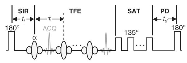
SIR-TFE pulse sequence diagram. The sequence employs i) a composite inversion pulse (Fig. 2) designed to uniformly invert M_zf over a range of expected ΔB₀ and B₁⁺ values with minimal macromolecular pool saturation, ii) a variable duration inversion recovery (SIR) period to sample the free pool recovery, iii) a TFE readout to efficiently cover k-space, iv) a pulse train to saturate (SAT) the free and macromolecular pools (allows t_d<5/λ⁻), and v) a predelay (PD) period to allow for partial M_z recovery. Legend: t_i = inversion time, t_d = predelay, τ = TFE pulse-to-pulse interval, ACQ = acquisition.

Plugging the initial condition of M_z(t_d=0)=0 into Eq. (4), signal equations can be generated for the predelay period of the SIR-TFE sequence. The ending values for this period can then be used as the initial condition for the inversion recovery period, taking account for the effect of the inversion pulse

$${\mathbf{M}}_z\left(t^{+}\right)={\mathbf{SM}}_2\left(t^{-}\right),$$ (6)

where S is a diagonal matrix with elements that account for the inversion of the free pool (S_f=−1 denotes complete inversion) and the saturation of the macromolecular pool (S_m=1 denotes no saturation) and t^+/− is the time immediately before/after the pulse. This yields the final expression for the evolution of M_z during the SIR period of the sequence

$${\mathbf{M}}_z(t_i,t_d)=\left(\exp \right({\mathbf{A}}_z{\mathbf{t}}_i\left)\mathbf{S}\right[\mathbf{I}-\exp \left({\mathbf{A}}_z{\mathbf{t}}_d\right)]+[\mathbf{I}-\exp \left({\mathbf{A}}_z{\mathbf{t}}_i\right)\left]\right){\mathbf{M}}_0.$$ (7)

In addition to these pulse sequence modifications, a novel 64-element composite inversion pulse was designed and employed herein to ensure a uniform inversion of M_zf over the range of B₁⁺ and ΔB₀ values previously measured in the human brain at 7.0 T (Moore et al., 2010). The optimization procedure (Moore et al., 2010) tended to produce high power pulses with suboptimal T₂-selectivity. As a result, we included an additional RF power constraint into the procedure, which was weighted against the uniform inversion constraint. The resulting amplitudes and phases of the subpulses are shown in Fig. 2. To evaluate the pulse’s performance, S_f and S_m were estimated from Eq. (6) by propagating Eq. (3) through each of the 64 subpulses [neglecting T₁ relaxation and MT during the pulse and assuming a Gaussian macromolecular pool lineshape with T_2m=10 μs (Gochberg and Gore, 2007)]. From this procedure, the pulse is predicted to yield a uniform inversion of M_zf over a wide range of B₁⁺ and ΔB₀ values without complete saturation of M_zm.

Fig. 2.

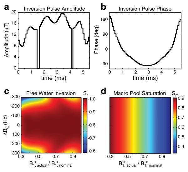
Composite inversion pulse amplitudes (a), phases (b), predicted free water inversion efficiency S_f (c), and predicted macromolecular saturation fractions S_m (d). S_f=−1 denotes complete inversion; S_m=1 denotes no saturation. The two zero-amplitude discontinuities in the RF pulse (a) are a consequence of the power constraint used in the minimization procedure. The RF phase (b) of the pulse at these discontinuities is arbitrary; therefore, the phase at these points was set based upon linear interpolation of the neighboring RF phases for display purposes.

Numerical simulations

The TFE readout employed herein effectively blurs the image along the phase-encoding direction according to its readout point-spread function (PSF), which is a complex function of the sequence timings and the NMR parameters of the tissue (Constable and Gore, 1992). If the readout PSF is constant as a function of t_i, then its effect will be to simply blur the final MT parameter maps. If, however, the readout PSF changes as a function of t_i, each image will be blurred to a different degree, potentially biasing the final parameter maps.

To evaluate this effect, the SIR-TFE signal arising from a one-dimensional (1D) test object was numerically simulated. As shown in Fig. 3, MT parameters were defined for test object regions representing white matter (WM), gray matter (GM), and cerebrospinal fluid (CSF). For each region and t_i, the signal evolution during each RF pulse and precession period of the TFE readout was simulated from Eq. (3) with the imaging parameters in the Data acquisition section—using M_z(t_i) from Eq. (7) as the initial condition and replacing each time-varying excitation pulse with a constant amplitude pulse of equivalent flip angle or root-mean-squared power (Ramani et al., 2002) for the free water or macromolecular pool, respectively. Complete spoiling of transverse magnetization was assumed prior to each RF pulse. The resulting M_zf immediately after each RF pulse was taken to represent the signal as a function of echo number. The signal was then re-ordered to account for the k-space trajectory and SENSE acceleration used, and the resulting re-ordered signal was taken to represent a k-space filter. To apply the k-space filters to the 1D test object, each uniform object region was Fourier transformed into k-space, multiplied by its corresponding k-space filter, and inverse Fourier transformed back into image space. The resulting object regions were then summed to generate the final blurred 1D object at each t_i. Finally, to assess the effect of the TFE readout on qMT parameter maps, the magnitude of the blurred test object signal at each voxel was fit to the M_zf component of Eq. (7) as described in the Data analysis section.

Fig. 3.

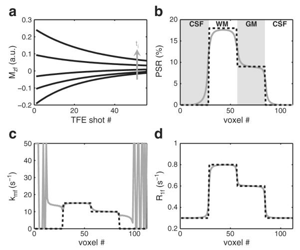
Numerical simulations of the SIR-TFE readout (a) and resulting qMT parameter fits for the 1D test object defined in (b–d). (a) The M_zf for each region (WM shown here) and t_i was simulated and reordered into the corresponding k-space filter. The resulting filters were applied to the 1D test object as described in the text. (b–d) From the simulated fit parameters (solid gray lines), it can be seen that the TFE readout blurs the parameter maps with little or no bias (except for k_mf in CSF regions, which do not exhibit an MT effect).

Subjects

MRI was performed on thirteen healthy volunteers (22–37 years old, 10 male, 3 female). To test reproducibility, six of the healthy volunteers were asked to undergo a second MRI scan at least two weeks after the first session. The study was approved by our local institutional review board, and signed consent was obtained prior to all examinations.

Data acquisition

Imaging was performed using a 7.0-T, Philips Achieva MR scanner (Philips Healthcare, Best, The Netherlands). A quadrature volume coil was used for excitation and a 32-channel head coil (Nova Medical, Wilmington, MA, USA) was used for signal reception. For qMT imaging, SIR-TFE data were collected in each subject using the general pulse sequence shown in Fig. 1.

An initial experiment was performed in one healthy volunteer to determine the effect of the post-TFE saturation train and predelay time t_d on the qMT parameter maps. For this initial experiment, SIR-TFE data were acquired in a single 5-mm axial slice with and without the post-TFE saturation train (see Fig. 1, shaded area labeled SAT) over a range of t_d values (0.125–10 s). Additional imaging parameters included: t_i logarithmically spaced between 6 ms and 2 s (15 values) and t_i=10 s, TFE echoes per shot=53, TFE pulse-to-pulse interval (τ)/TE/α=2.8 ms/1.4 ms/15°, SENSE factor=2, field-of-view=212×212 mm², resolution=2.0×2.0 mm², and number of signal acquisitions averaged (NSA)=2.

Based upon the results of this experiment along with previous numerical simulations (Gochberg and Gore, 2007), a t_d of 2.5 s was chosen to balance the scan time and SNR constraints for whole-brain SIR-TFE imaging. Whole-brain qMT data were acquired in 12 volunteers (six scanned twice) via a three-dimensional (3D) SIR-TFE sequence using the previously listed parameters except: t_i logarithmically spaced between 6 ms and 2 s (13 values) and t_i=8 s, SENSE factor=4 (2 anteri-or–posterior, 2 superior–inferior), field-of-view=212×212×90 mm³, resolution=2.0×2.0×3.0 mm³, and NSA=1. This resulted in an acquisition time≈19 min for 30 slices.

Recall that the signal model [Eq. (7)] has terms (S_f and S_m) that account for the effect of the inversion pulse on the free and macromolecular pool magnetizations. S_f was included as a free parameter in the fit as described in the Data analysis section, while S_m was numerically estimated as described in the Pulse sequence section. Because S_m is sensitive to B₁⁺ (see Fig. 2d), this numerical estimation required an independent measurement of B₁⁺. As a result, B₁⁺ was estimated in same volume as the SIR-TFE data using the actual flip angle imaging (AFI) method (Yarnykh, 2007) with TR₁/TR₂=125/25 ms and a 60° slab-selective excitation pulse (asymmetric sinc pulse with Gaussian apodization).

Data analysis

All data analyses were performed in MATLAB (Mathworks, Natick, MA). Prior to data fitting, each SIR-TFE and AFI volume was co-registered to the SIR-TFE volume acquired at t_i=110 ms (middle value) using a 3D rigid body registration based upon normalized mutual information (Viola and Wells, 1997). Following co-registration, automatic brain extraction was performed (Smith, 2002) and qMT parameter maps were calculated in each volunteer. The SIR-TFE signal model described in Eq. (7) has seven independent parameters: R_1m, R_1f, S_m, S_f, M_0f, PSR=M_0m/M_0f, and k_mf (k_fm=k_mfPSR). As is the case with pulsed saturation methods, the signal dependence on R_1m for SIR data is weak (Li et al., 2010). Therefore, R_1m was set equal to R_1f for fitting purposes. The parameter S_m was numerically estimated for each voxel. This required an independent estimate of the actual flip angle in each voxel (α_actual), which was calculated from the AFI data using the following relationship (Yarnykh, 2007):

$${\alpha }_{\text{actual}}={\cos }^{-1}\left(\frac{\mathit{rn}-1}{n-r}\right),$$ (8)

where n=TR₂/TR₁, r=S(TR₂)/S(TR₂), and S is the signal intensity. The resulting α_actual map was smoothed with a 10×10×9 mm³ moving-average filter to minimize the impact of imaging artifacts. Following this operation, the flip angle values were converted to B_1,actual⁺ values for the composite inversion pulse (see Fig. 2a) and S_m was estimated using the procedure described in the Pulse sequence section (see Fig. 2d). The remaining five parameters (R_1f, S_f, M_0f, k_mf, and PSR) were estimated for each voxel by fitting SIR-TFE data (14 t_i values) to the M_zf component of Eq. (7) in a least-squares sense using the procedure described in Dortch et al. (2011).

SIR-TFE data had a mean SNR per voxel of 180±50 (range=60–320) within the defined ROIs, where SNR is defined as M_0f divided by the standard deviation (SD) of the residuals of the fit. Monte Carlo simulations, similar to those described by Li et al. (2010), were performed to predict the uncertainty of the fit parameters at these SNR levels. The t_i and t_d values listed above were used for these simulations. Additional simulation parameters included: R_1m=R_1f=0.8 s⁻¹, k_mf=15 s⁻¹, PSR=15%, S_m=0.7, and S_f=−0.95. Over an SNR range of 60–320, the SDs of the fit PSR, R_1f, and k_mf values were 0.4–2.2%, 0.01–0.03 s⁻¹, and 0.9–5.5 s⁻¹, respectively. This suggests that PSR and R_1f can be robustly determined from the in vivo brain data collected herein. Consistent with previous studies (Li et al., 2010), the uncertainty in k_mf is expected to be much larger, especially in lower SNR regions.

Following this fitting procedure, qMT parameter maps were smoothed with a locally-adaptive Gaussian filter (kernel size=10×10×9 mm³, full width at half maximum=1/2 kernel size) to remove outliers that tended to occur at tissue boundaries. To perform this operation, each filtered map was subtracted from the raw parameter map, and outliers were defined as voxels whose value was three standard deviations above the mean difference across all voxels. For these outliers, the value in the raw parameter map was replaced with the value in the filtered map. This process was iterated until the number of outliers was less than the expected value (0.3% of the total number of voxels).

Statistics

Mean qMT parameters (PSR, R_1f, and k_mf) were calculated within the following regions-of-interest (ROI): head of the caudate, putamen, thalamus, genu and splenium of the corpus callosum, internal capsule, corona radiata, occipital WM, and frontal WM. Statistical comparisons were performed on the mean ROI values to evaluate each parameter’s i) variation across ROIs (i.e., regional differences), ii) variation and reproducibility across time, and iii) variation across volunteers. To compare parameters across WM regions, a non-parametric Wilcoxon rank-sum test was performed, with a p<0.05 deeming a significant difference between ROI values. To evaluate the test–retest reproducibility of each parameter, a Bland–Altman (BA) analysis was performed. For the BA analysis, the mean difference and the limits of agreement (LOA=mean difference±1.96*SD) were tabulated across scans for all ROIs. Additionally, a Wilcoxon signed-rank test was performed between the test and retest parameter values for each ROI, with a p>0.05 indicating a non-significant difference between scans at each time point. To assess the test–retest variability of each parameter within each ROI, the coefficient of variation was calculated from: ${\mathit{CV}}_{\text{retest}}=S∕\left(M\sqrt{2}\right)\ast 100$, where S is the SD of the test–retest difference across subjects, M is the mean value across all test–retest scans and subjects, and the $\sqrt{2}$ term accounts for the propagation of uncertainty from the difference operation. The across-cohort variability of each parameter within each ROI was also assessed via: CV_cohort =S/M*100, where S is the SD across the cohort and M is mean value across the cohort. All values are reported as the mean±SD unless otherwise stated.

Results

The results of the numerical simulations designed to assess the effect of TFE readout on qMT parameter maps are shown in Fig. 3. In Fig. 3a, the evolution of M_zf during the TFE readout is shown for WM as a function of t_i. Note that this evolution is related to the k-space filter of the readout. It can be seen that the shape (width and rate of decay) of the k-space filter changes as a function of t_i, which manifests as a change in object blurring as a function of t_i. The effect of this on the qMT parameter maps is shown in Figs. 3b–d. It can be seen that the resulting qMT parameter maps are smoothed in the phase-encoding direction with little bias in the fit parameters. It should be noted, however, that PSR values were slightly underestimated in the WM region of the 1D test object. Additional simulations indicated that this bias increased as the size of the WM region decreased.

Fig. 4 displays PSR maps acquired with and without application of the post-TFE saturation train (see the SAT region in Fig. 1) as a function of t_d. For scans with the saturation train, the fit PSR values at shorter t_d values were nearly identical to those at full recovery (t_d=10 s). Without this train, small deviations in PSR were observed at t_d=2.5 s; and these were more pronounced at t_d=1.25 s. Thus, the post-TFE saturation train allows for reduction of t_d (and scan times) with minimal parameter bias.

Fig. 4.

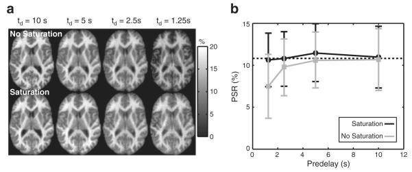
(a) Maps of PSR as a function of t_d without (top) and with (bottom) a post-TFE saturation train and (b) corresponding mean (±SD) slice-wise PSR values. For scans with the saturation train, all PSR values were nearly identical to the values at full recovery (dashed line). Without the saturation train, PSR values were increasingly underestimated with decreasing t_d.

Representative 3D SIR-TFE data are shown in Fig. 5. Fig. 5a shows a single slice at the level of the lateral ventricles acquired at six of 14 t_i values. Note the characteristic center brightening due to B₁⁺ inhomogeneities. Fig. 5b shows data from a single voxel in the genu of the corpus callosum and the corresponding model fit. Note the agreement between the SIR-TFE data and the biexponential model described by Eq. (7). Additionally, note the deviation from monoexponential recovery, which is especially evident at the shortest inversion times.

Fig. 5.

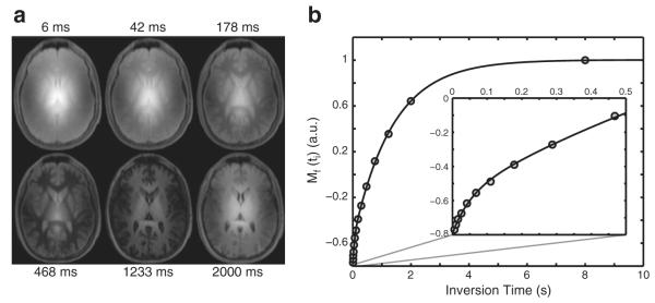
Sample SIR-TFE images (a) and model fit (b) from a slice at the level of the lateral ventricles in a healthy control. (a) Images from six of the 14 inversion times are shown. Note the characteristic center brightening of the images due to B₁⁺ inhomogeneities. (b) Corresponding SIR data from a voxel in the genu of the corpus callosum. Note the agreement between the SIR data (circles) and biexponential model [solid black line, Eq. (7)] and the deviation from a monoexponential model, which is apparent at the shortest inversion times shown in the zoomed inset.

Based upon these fits, maps of qMT parameters were generated. Recall that these maps were filtered to reduce the impact of outliers.Fig. 6 displays representative qMT parameter maps without filtering, with the previously described locally-adaptive Gaussian filter, and with a global Gaussian filter. The locally-adaptive and global filters both removed outliers in the parameter maps (see arrow in the top row and the masks in the bottom row); however, the locally filtered maps were blurred to a much smaller degree. As a result, we employed the locally-adaptive approach herein. For all parameter maps, 14% of all voxels in the post-brain-extraction volume were smoothed using this approach. However, as seen in the bottom row of Fig. 6, a majority of these voxels were located along the brain surface or within the CSF.

Fig. 6.

Representative qMT parameter (PSR, k_mf, R_1f) maps with and without filtering. Shown are (1st row) raw parameter maps, (2nd row) parameter maps filtered with the locally-adaptive Gaussian filter, (3rd row) parameter maps filtered with the global Gaussian filter (with an identical kernel), and (4th row) masks of the outliers detected using the locally-adaptive filter. The arrow identifies a region with biased PSR values that are corrected by filtering. Note that the color-scale in these maps was chosen to highlight the outliers and is different than in Figs. 4 and 8.

Fig. 7 displays results from four representative slices in one healthy subject. The qMT parameters were uniform over most of the volume despite the presence of large ΔB₀ and/or B₁⁺ field inhomogeneities (as indicated by the heterogeneity in the S_m maps). There does, however, appear to be some bias in the qMT parameter values in midbrain slices (black arrow), which typically (Moore et al., 2010) exhibit the largest field inhomogeneities and the lowest SNR. Nevertheless, these data suggest that robust qMT parameter mapping can be achieved throughout most of the brain using the 3D SIR-TFE protocol described herein.

Fig. 7.

Representative parameter maps from one subject (four of 30 slices are shown). The qMT parameters (PSR, k_mf, R_1f) and the inversion efficiency S_f were uniform over most of the volume despite the presence of large field inhomogeneities. There does, however, appear to be some bias in the qMT parameter values in midbrain slices (black arrows), which typically exhibit the largest B₀ and B₁⁺ inhomogeneities. This results in a deviation of S_f from −1 in these regions.

ROIs were defined in a number of WM and GM regions as shown in Fig. 8. The boxplots in the top row of Fig. 9 display the mean ROI qMT parameters over the 12 healthy volunteers. For PSR, the mean value across all WM ROIs (17.6±1.3%) was higher than the values across all GM ROIs (10.3±1.6%). Additionally, heterogeneity within WM PSR values was observed, but should be interpreted with caution due to the effect of multiple comparisons. Nevertheless, differences between the following regions were detected: i) the genu of the corpus callosum and occipital WM (p=0.026), ii) the genu of the corpus callosum and the corona radiata (p=0.026), iii) frontal and occipital WM (p=0.041), and iv) frontal WM and the corona radiata (p=0.041). Fit k_mf values were higher in GM (24.4±4.4 s⁻¹) than in WM (14.5±1.5 s⁻¹). Additionally, note the large, biased k_mf values in and around areas containing CSF, which is likely a consequence of the weak dependence of the signal on k_mf when PSR≈0 (see the simulated data in Fig. 3c). For R_1f, differences between WM (0.73±0.03 s⁻¹) and GM (0.58±0.05 s⁻¹) values were also observed. The boxplots in Fig. 9 give an indication of the variability of each parameter across the healthy cohort. To quantify this, the coefficient of variation was tabulated for each ROI, and the mean value across all ROI is given in Table 1. From this, it can be seen that the mean CV_cohort was <10% for all of the qMT parameters, which is not surprising given the small age range of the healthy cohort scanned herein.

Fig. 8.

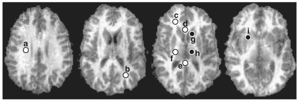
Representative PSR maps from a single volunteer with corresponding ROIs (a=corona radiata; b=occipital WM; c=frontal WM; d=corpus callosum, genu; e=corpus callosum, splenium; f=internal capsule; g=head of caudate; h=thalamus; i=putamen). White and black dots represent WM and GM ROIs, respectively. In practice, ROIs were defined bilaterally and results were averaged across hemispheres. Here we show ROIs in one hemisphere for display purposes.

Fig. 9.

(a–c) Boxplot of the mean ROI qMT parameters (hc = head of caudate; put = putamen; thal = thalamus; owm = occipital WM; scc = corpus callosum, splenium; ic = internal capsule; cr = corona radiata; gcc = corpus callosum, genu; fwm = frontal WM). On each box, the central mark is the median, the edges of the box are the 25th and 75th percentiles, and the whiskers extend to the most extreme data points. (d–f) Bland–Altman plots of the difference in parameters for WM (black) and GM (gray) ROIs across scans. The solid line is the mean difference, and the dashed lines are the limits of agreement (mean difference±1.96 SD).

Table 1.

Test–retest reproducibility analysis of each qMT parameter (PSR, R_1f, and k_mf). Shown are the mean±SD parameter values across all ROIs for the test and retest scans, the resulting mean paired-difference between time-points, the limits-of-agreement (LOA), and the mean±SD test–retest coefficient of variation (CVretest) across all ROIs. For comparison, the corresponding across-cohort coefficient of variation (CVcohort) is also given.

Parameter	Test scan (mean±SD)	Retest scan (mean±SD)	Difference	LOA	CVretest (%)	CVcohort (%)
PSR (%)	15.2±3.9	15.2±3.7	0.0	(−2.2, 2.1)	4.9±1.5	5.6±1.9
kmf (s−1)	16.8±4.7	18.0±5.5	1.2	(−3.9, 6.3)	8.2±2.4	9.4±3.6
R −1f (s 1)	0.68±0.08	0.68±0.08	0.01	(−0.03, 0.04)	1.9±1.4	3.2±1.3

BA plots of the observed difference in mean ROI qMT parameters between scans are shown in the bottom row of Fig. 9; and the results from this analysis are given numerically in Table 1. The mean difference for all ROIs across scans was close to zero for PSR (0.0%), k_mf (1.2 s⁻¹), and R_1f (0.01 s⁻¹), indicating a lack of bias and reasonable reproducibility. To further test this, a Wilcoxon signed-rank test was performed on the test–retest parameter values in each ROI. At the p=0.05 level, no significant difference was observed between test and retest qMT parameters in any of the ROIs except for k_mf in the genu of the corpus callosum (p=0.031). The test–retest coefficient of variation (CV_retest) was also tabulated for each metric to further assess each parameter’s variability across time. As shown in Table 1, the relative CV_retest values were consistent with the corresponding CV_cohort values, with k_mf exhibiting the highest variability. In terms of absolute CV values, the test–retest variability was approximately 20% lower than the across cohort variability.

Discussion

This study demonstrates the feasibility of performing whole-brain qMT measurements in the human brain in vivo at high field. Pulsed saturation and SSFP-based approaches are difficult to implement at high field due to RF power limitations and/or magnetic field (B₁⁺ and ΔB₀) inhomogeneities. In this study, we employed the SIR qMT approach, which has been suggested to be less sensitive to these issues. The biggest obstacles to overcome were i) the effect of B₁⁺ and ΔB₀ inhomogeneities on the inversion pulse and the readout and ii) the long scan times associated with SIR imaging. The former of these was mitigated by developing a novel B₁⁺ and ΔB₀ insensitive inversion composite pulse (Fig. 2) and employing a low-flip angle TFE readout; the latter was mitigated by the efficiency of the TFE readout along with additional protocol optimization (e.g., reducing the number of t_I values to 14, applying SENSE acceleration in two directions). Together this resulted in a robust (Fig. 9), whole-brain qMT imaging protocol with a scan time of less than 20 min.

Previous qMT imaging studies at lower field strengths (Dortch et al., 2011; Garcia et al., 2010; Gloor et al., 2008; Ropele et al., 2003; Sled and Pike, 2001; Sled et al., 2004; Yarnykh and Yuan, 2004) have reported PSR values in the range of 11–16% and 5–9% for WM and GM structures, respectively [PSR=F using the notation of Sled and Pike (2000, 2001) and M_0b using the notation of Henkelman et al. (1993)]. The PSR values presented herein (WM: 15–20%, GM: 9–13%) were approximately 25% higher. PSR should be independent of field strength, so these differences may be related to the SIR-TFE sequence. As previously discussed, we modified the inversion pulse and readout of our 3.0-T SIR-FSE sequence to perform qMT imaging at 7.0 T. The effect of the TFE readout on the fit qMT parameters was assessed via numerical simulations and was found to result in little bias in PSR (Fig. 3). However, it should be noted that our previous report at 3.0 T employed a much longer TE (74 ms) than was employed herein (1.4 ms). Previous work (Bjarnason et al., 2005; Stanisz et al., 1999) has demonstrated that MT contrast is TE-dependent in WM due to the microanatomical compartition of water into myelin and nonmyelin water spaces. As a result, it is reasonable to assume that PSR may also exhibit a TE-dependence. In terms of the inversion pulse, we recognize that PSR is sensitive to the macromolecular pool lineshape and T_2m assumptions used in the numerical estimation of S_m. Similar to our previous studies (Dortch et al., 2011; Gochberg and Gore, 2007), we modeled the macromolecular pool using a Gaussian lineshape (T_2m=10 μs) because the Super-Lorentzian exhibits an on-resonance singularity. Previous work using a 1-ms block inversion pulse at 3.0 T (Dortch et al., 2011) found that this was a reasonable approximation; however, this may not be true for the longer (5.5 ms), higher power composite inversion pulse employed herein. Additional work is needed to explore the field- and TE-dependence of PSR values obtained via the SIR technique. Nevertheless, the reported regional variation in PSR values was consistent with previous qMT imaging studies (Dortch et al., 2011; Garcia et al., 2010; Sled et al., 2004; Underhill et al., 2009); and additional SIR-TFE studies in bovine serum albumin phantoms at 7.0 T (data not shown) found a linear relationship between macromolecular content and PSR. Thus, we postulate that the regional differences in PSR values reported herein are driven primarily by regional differences in myelin content, although the absolute values may be systematically larger than reported by other techniques.

Previous pulsed saturation and SSFP-based studies (Garcia et al., 2010; Gloor et al., 2008; Ropele et al., 2003; Sled and Pike, 2001; Sled et al., 2004; Yarnykh and Yuan, 2004) report k_mf values [k_mf=k_f/F using the notation of Sled and Pike (2000, 2001); k_mf=R when M_0f=1 using the notation of Henkelman et al. (1993)] in the range of 20–40 s⁻¹ across the brain. A previous SIR study (Dortch et al., 2011) at 3.0 T reports k_mf values that are approximately 2-fold slower (10–15 s^—1) with values that are slower in WM than GM, which is consistent with the results presented herein. The discrepancies between techniques are not surprising given the reported difficulty of using pulsed saturation to determine k_mf (Portnoy and Stanisz, 2007). In terms of the current study, it should be noted that k_mf showed the largest variability of the qMT parameters, which is consistent with the results from the Monte Carlo simulations. We do not expect this to be a significant drawback as k_mf has been shown to be insensitive to the pathological changes in spinal cord WM (Smith et al., 2009).

While there have been no previous reports of R_1f in human brain at 7.0 T, it can be shown that the observed T₁ typically reported is≈1/R_1f. Using this relationship, the mean WM and GM observed T₁ values were 1372 and 1724 ms, respectively, which are within the range of previously reported values in human brain at 7.0 T (Wright et al., 2008). As expected, we noted a significant correlation between R_1f and PSR in the healthy human brain (data not shown); however, T₁ is sensitive to overall tissue composition [e.g., water content (Kiricuta and Simplaceanu, 1975)] and is believed to be a less specific marker for myelin in WM.

The increased SNR available at 7.0 T was used here to decrease scan time (≈40 s/slice) and increase resolution (2×2×3 mm³) relative to our 3.0-T protocol. Moving forward, it may be advantageous to look at higher resolution protocols. If we assume that all imaging parameters are the same, increasing the resolution to 1×1×3 mm³ would result in an approximately two-fold decrease in SNR (≈70 at thermal equilibrium, assuming we increase the number of acquired points to hold the field-of-view constant). Based upon previous simulation work (Li et al., 2010) as well as the simulation work presented herein, this would be sufficient to robustly fit qMT parameters over most of the brain. Thus, it appears that high-resolution qMT imaging may be feasible in the human brain in vivo at 7.0 T using a protocol similar to that described herein.

Conclusions

The results of this study demonstrate the feasibility of performing qMT imaging in human brain in vivo at high field. The developed SIR-TFE protocol allowed for whole-brain qMT imaging in less than 20 min. In healthy subjects, intra-subject reliability (i.e., test–retest) was demonstrated despite large ΔB₀ and B₁⁺ variations. Additionally, a high level of inter-subject reproducibility was demonstrated for the qMT parameters. Future work includes investigating high-resolution protocols to look at cortical features of qMT parameters and application of the approach in a cohort of multiple sclerosis patients.

References

- Berry I, Barker G, Barkhof F, Campi A, Dousset V, Franconi J, Gass A, Schreiber W, Miller D, Tofts P. A multicenter measurement of magnetization transfer ratio in normal white matter. J. Magn. Reson. Imaging. 1999;9:441–446. doi: 10.1002/(sici)1522-2586(199903)9:3<441::aid-jmri12>3.0.co;2-r. [DOI] [PubMed] [Google Scholar]
- Bjarnason T, Vavasour I, Chia C, Mackay A. Characterization of the NMR behavior of white matter in bovine brain. Magn. Reson. Med. 2005;54:1072–1081. doi: 10.1002/mrm.20680. [DOI] [PubMed] [Google Scholar]
- Bruno SD, Barker GJ, Cercignani M, Symms M, Ron MA. A study of bipolar disorder using magnetization transfer imaging and voxel-based morphometry. Brain. 2004;127:2433–2440. doi: 10.1093/brain/awh274. [DOI] [PubMed] [Google Scholar]
- Catalaa I, Grossman RI, Kolson DL, Udupa JK, Nyul LG, Wei L, Zhang X, Polansky M, Mannon LJ, McGowan JC. Multiple sclerosis: magnetization transfer histogram analysis of segmented normal-appearing white matter. Radiology. 2000;216:351–355. doi: 10.1148/radiology.216.2.r00au16351. [DOI] [PubMed] [Google Scholar]
- Cercignani M, Alexander D. Optimal acquisition schemes for in vivo quantitative magnetization transfer MRI. Magn. Reson. Med. 2006;56:803–810. doi: 10.1002/mrm.21003. [DOI] [PubMed] [Google Scholar]
- Constable RT, Gore JC. The loss of small objects in variable TE imaging: implications for FSE, RARE, and EPI. Magn. Reson. Med. 1992;28:9–24. doi: 10.1002/mrm.1910280103. [DOI] [PubMed] [Google Scholar]
- Dortch RD, Li K, Gochberg DF, Welch EB, Dula AN, Tamhane AA, Gore JC, Smith SA. Quantitative magnetization transfer imaging in human brain at 3 T via selective inversion recovery. Magn. Reson. Med. 2011;66:1346–1352. doi: 10.1002/mrm.22928. [DOI] [PMC free article] [PubMed] [Google Scholar]
- Dousset V, Grossman RI, Ramer KN, Schnall MD, Young LH, Gonzalez-Scarano F, Lavi E, Cohen JA. Experimental allergic encephalomyelitis and multiple sclerosis: lesion characterization with magnetization transfer imaging. Radiology. 1992;182:483–491. doi: 10.1148/radiology.182.2.1732968. [DOI] [PubMed] [Google Scholar]
- Edzes HT, Samulski ET. Cross relaxation and spin diffusion in the proton NMR or hydrated collagen. Nature. 1977;265:521–523. doi: 10.1038/265521a0. [DOI] [PubMed] [Google Scholar]
- Filippi M, Rocca MA. Magnetization transfer magnetic resonance imaging in the assessment of neurological diseases. J. Neuroimaging. 2004;14:303–313. doi: 10.1177/1051228404265708. [DOI] [PubMed] [Google Scholar]
- Garcia M, Gloor M, Wetzel SG, Radue E-W, Scheffler K, Bieri O. Characterization of normal appearing brain structures using high-resolution quantitative magnetization transfer steady-state free precession imaging. NeuroImage. 2010;52:532–537. doi: 10.1016/j.neuroimage.2010.04.242. [DOI] [PubMed] [Google Scholar]
- Gass A, Barker GJ, Kidd D, Thorpe JW, MacManus D, Brennan A, Tofts PS, Thompson AJ, McDonald WI, Miller DH. Correlation of magnetization transfer ratio with clinical disability in multiple sclerosis. Ann. Neurol. 1994;36:62–67. doi: 10.1002/ana.410360113. [DOI] [PubMed] [Google Scholar]
- Gloor M, Scheffler K, Bieri O. Quantitative magnetization transfer imaging using balanced SSFP. Magn. Reson. Med. 2008;60:691–700. doi: 10.1002/mrm.21705. [DOI] [PubMed] [Google Scholar]
- Gochberg D, Gore J. Quantitative magnetization transfer imaging via selective inversion recovery with short repetition times. Magn. Reson. Med. 2007;57:437–441. doi: 10.1002/mrm.21143. [DOI] [PMC free article] [PubMed] [Google Scholar]
- Gochberg D, Kennan R, Gore J. Quantitative studies of magnetization transfer by selective excitation and T1 recovery. Magn. Reson. Med. 1997;38:224–231. doi: 10.1002/mrm.1910380210. [DOI] [PubMed] [Google Scholar]
- Graham SJ, Henkelman RM. Understanding pulsed magnetization transfer. J. Magn. Reson. Imaging. 1997;7:903–912. doi: 10.1002/jmri.1880070520. [DOI] [PubMed] [Google Scholar]
- Henkelman R, Huang X, Xiang Q, Stanisz G, Swanson S, Bronskill M. Quantitative interpretation of magnetization transfer. Magn. Reson. Med. 1993;29:759–766. doi: 10.1002/mrm.1910290607. [DOI] [PubMed] [Google Scholar]
- Kabani NJ, Sled JG, Chertkow H. Magnetization transfer ratio in mild cognitive impairment and dementia of Alzheimer’s type. NeuroImage. 2002a;15:604–610. doi: 10.1006/nimg.2001.0992. [DOI] [PubMed] [Google Scholar]
- Kabani NJ, Sled JG, Shuper A, Chertkow H. Regional magnetization transfer ratio changes in mild cognitive impairment. Magn. Reson. Med. 2002b;47:143–148. doi: 10.1002/mrm.10028. [DOI] [PubMed] [Google Scholar]
- Kalkers NF, Hintzen RQ, van Waesberghe JH, Lazeron RH, van Schijndel RA, Ader HJ, Polman CH, Barkhof F. Magnetization transfer histogram parameters reflect all dimensions of MS pathology, including atrophy. J. Neurol. Sci. 2001;184:155–162. doi: 10.1016/s0022-510x(01)00431-2. [DOI] [PubMed] [Google Scholar]
- Kiricuta IC, Jr., Simplaceanu V. Tissue water content and nuclear magnetic resonance in normal and tumor tissues. Cancer Res. 1975;35:1164–1167. [PubMed] [Google Scholar]
- Koenig SH. Cholesterol of myelin is the determinant of gray–white contrast in MRI of brain. Magn. Reson. Med. 1991;20:285–291. doi: 10.1002/mrm.1910200210. [DOI] [PubMed] [Google Scholar]
- Kucharczyk W, Macdonal P, Stanisz G, Henkelman R. Relaxivity and magnetization transfer of white matter lipids at MR imaging: importance of cerebrosides and pH. Radiology. 1994;192:521–529. doi: 10.1148/radiology.192.2.8029426. [DOI] [PubMed] [Google Scholar]
- Levesque IR, Sled JG, Pike GB. Iterative optimization method for design of quantitative magnetization transfer imaging experiments. Magn. Reson. Med. 2011;66:635–643. doi: 10.1002/mrm.23071. [DOI] [PubMed] [Google Scholar]
- Li K, Zu Z, Xu J, Janve VA, Gore JC, Does MD, Gochberg DF. Optimized inversion recovery sequences for quantitative T1 and magnetization transfer imaging. Magn. Reson. Med. 2010;64:491–500. doi: 10.1002/mrm.22440. [DOI] [PMC free article] [PubMed] [Google Scholar]
- Moore J, Jankiewicz M, Zeng H, Anderson AW, Gore JC. Composite RF pulses for B1+-insensitive volume excitation at 7 Tesla. J. Magn. Reson. 2010;205:50–62. doi: 10.1016/j.jmr.2010.04.002. [DOI] [PMC free article] [PubMed] [Google Scholar]
- Morrison C, Stanisz G, Henkelman RM. Modeling magnetization transfer for biological-like systems using a semi-solid pool with a super-Lorentzian lineshape and dipolar reservoir. J. Magn. Reson. B. 1995;108:103–113. doi: 10.1006/jmrb.1995.1111. [DOI] [PubMed] [Google Scholar]
- Mougin OE, Coxon RC, Pitiot A, Gowland PA. Magnetization transfer phenomenon in the human brain at 7 T. NeuroImage. 2010;49:272–281. doi: 10.1016/j.neuroimage.2009.08.022. [DOI] [PubMed] [Google Scholar]
- Mugler JP, III, Brookeman JR. Three-dimensional magnetization-prepared rapid gradient-echo imaging (3D MP RAGE) Magn. Reson. Med. 1990;15:152–157. doi: 10.1002/mrm.1910150117. [DOI] [PubMed] [Google Scholar]
- Odrobina E, Lam T, Pun T, Midha R, Stanisz G. MR properties of excised neural tissue following experimentally induced clemyelination. NMR Biomed. 2005;18:277–284. doi: 10.1002/nbm.951. [DOI] [PubMed] [Google Scholar]
- Ou X, Sun SW, Liang HF, Song SK, Gochberg DF. The MT pool size ratio and the DTI radial diffusivity may reflect the myelination in shiverer and control mice. NMR Biomed. 2009;22:480–487. doi: 10.1002/nbm.1358. [DOI] [PMC free article] [PubMed] [Google Scholar]
- Pike GB. Pulsed magnetization transfer contrast in gradient echo imaging: a two-pool analytic description of signal response. Magn. Reson. Med. 1996;36:95–103. doi: 10.1002/mrm.1910360117. [DOI] [PubMed] [Google Scholar]
- Portnoy S, Stanisz GJ. Modeling pulsed magnetization transfer. Magn. Reson. Med. 2007;58:144–155. doi: 10.1002/mrm.21244. [DOI] [PubMed] [Google Scholar]
- Ramani A, Dalton C, Miller DH, Tofts PS, Barker GJ. Precise estimate of fundamental in-vivo MT parameters in human brain in clinically feasible times. Magn. Reson. Imaging. 2002;20:721–731. doi: 10.1016/s0730-725x(02)00598-2. [DOI] [PubMed] [Google Scholar]
- Ropele S, Seifert T, Enzinger C, Fazekas F. Method for quantitative imaging of the macromolecular 1H fraction in tissues. Magn. Reson. Med. 2003;49:864–871. doi: 10.1002/mrm.10427. [DOI] [PubMed] [Google Scholar]
- Schmierer K, Scaravilli F, Altmann D, Barker G, Miller D. Magnetization transfer ratio and myelin in postmortem multiple sclerosis brain. Ann. Neurol. 2004;56:407–415. doi: 10.1002/ana.20202. [DOI] [PubMed] [Google Scholar]
- Schmierer K, Tozer DJ, Scaravilli F, Altmann DR, Barker GJ, Tofts PS, Miller DH. Quantitative magnetization transfer imaging in postmortem multiple sclerosis brain. J. Magn. Reson. Imaging. 2007;26:41–51. doi: 10.1002/jmri.20984. [DOI] [PMC free article] [PubMed] [Google Scholar]
- Sled JG, Pike GB. Quantitative interpretation of magnetization transfer in spoiled gradient echo MRI sequences. J. Magn. Reson. 2000;145:24–36. doi: 10.1006/jmre.2000.2059. [DOI] [PubMed] [Google Scholar]
- Sled JG, Pike GB. Quantitative imaging of magnetization transfer exchange and relaxation properties in vivo using MRI. Magn. Reson. Med. 2001;46:923–931. doi: 10.1002/mrm.1278. [DOI] [PubMed] [Google Scholar]
- Sled JG, Levesque I, Santos AC, Francis SJ, Narayanan S, Brass SD, Arnold DL, Pike GB. Regional variations in normal brain shown by quantitative magnetization transfer imaging. Magn. Reson. Med. 2004;51:299–303. doi: 10.1002/mrm.10701. [DOI] [PubMed] [Google Scholar]
- Smith SM. Fast robust automated brain extraction. Hum. Brain Mapp. 2002;17:143–155. doi: 10.1002/hbm.10062. [DOI] [PMC free article] [PubMed] [Google Scholar]
- Smith S, Golay X, Fatemi A, Mahmood A, Raymond G, Moser H, van Zijl P, Stanisz G. Quantitative magnetization transfer characteristics of the human cervical spinal cord in vivo: application to adrenomyeloneuropathy. Magn. Reson. Med. 2009;61:22–27. doi: 10.1002/mrm.21827. [DOI] [PMC free article] [PubMed] [Google Scholar]
- Stanisz G, Kecojevic A, Bronskill M, Henkelman R. Characterizing white matter with magnetization transfer and T2. Magn. Reson. Med. 1999;42:1128–1136. doi: 10.1002/(sici)1522-2594(199912)42:6<1128::aid-mrm18>3.0.co;2-9. [DOI] [PubMed] [Google Scholar]
- Underhill HR, Yuan C, Yarnykh VL. Direct quantitative comparison between cross-relaxation imaging and diffusion tensor imaging of the human brain at 3.0 T. NeuroImage. 2009;47:1568–1578. doi: 10.1016/j.neuroimage.2009.05.075. [DOI] [PubMed] [Google Scholar]
- Underhill HR, Rostomily RC, Mikheev AM, Yuan C, Yarnykh VL. Fast bound pool fraction imaging of the in vivo rat brain: association with myelin content and validation in the C6 glioma model. NeuroImage. 2011;54:2052–2065. doi: 10.1016/j.neuroimage.2010.10.065. [DOI] [PMC free article] [PubMed] [Google Scholar]
- Viola P, Wells WM. Alignment by maximization of mutual information. Int. J. Comput. Vis. 1997;24:137–154. [Google Scholar]
- Wolff SD, Balaban RS. Magnetization transfer contrast (MTC) and tissue water proton relaxation in vivo. Magn. Reson. Med. 1989;10:135–144. doi: 10.1002/mrm.1910100113. [DOI] [PubMed] [Google Scholar]
- Wright PJ, Mougin OE, Totman JJ, Peters AM, Brookes MJ, Coxon R, Morris PE, Clemence M, Francis ST, Bowtell RW, Gowland PA. Water proton T1 measurements in brain tissue at 7, 3, and 1.5 T using IR-EPI, IR-TSE, and MPRAGE: results and optimization. MAGMA. 2008;21:121–130. doi: 10.1007/s10334-008-0104-8. [DOI] [PubMed] [Google Scholar]
- Yarnykh VL. Actual flip-angle imaging in the pulsed steady state: a method for rapid three-dimensional mapping of the transmitted radiofrequency field. Magn. Reson. Med. 2007;57:192–200. doi: 10.1002/mrm.21120. [DOI] [PubMed] [Google Scholar]
- Yarnykh VL, Yuan C. Cross-relaxation imaging reveals detailed anatomy of white matter fiber tracts in the human brain. NeuroImage. 2004;23:409–424. doi: 10.1016/j.neuroimage.2004.04.029. [DOI] [PubMed] [Google Scholar]