Susceptibility Gradient Mapping (SGM): A New Postprocessing Method for Positive Contrast Generation Applied to Superparamagnetic Iron Oxide Particle (SPIO)-Labeled Cells

Abstract

Local susceptibility gradients result in a dephasing of the precessing magnetic moments and thus in a fast decay of the NMR signals. In particular, cells labeled with superparamagnetic iron oxide particles (SPIOs) induce hypointensities, making the in vivo detection of labeled cells from such a negative image contrast difficult. In this work, a new method is proposed to selectively turn this negative contrast into a positive contrast. The proposed method calculates the susceptibility gradient and visualizes it in a parametric map directly from a regular gradient-echo image dataset. The susceptibility gradient map is determined in a postprocessing step, requiring no dedicated pulse sequences or adaptation of the sequence before and during image acquisition. Phantom experiments demonstrated that local susceptibility differences can be quantified. In vivo experiments showed the feasibility of the method for tracking of SPIO-labeled cells. The method bears the potential also for usage in other applications, including the detection of contrast agents and interventional devices as well as metal implants.

MRI is based upon the use of a homogeneous static magnetic field for the detection of coherently precessing magnetic moments. Usually, a homogeneity in the range of parts per million (ppm) is required to measure an NMR signal. Any local inhomogeneity in the static magnetic field results in the dephasing of the precessing magnetic moments, and thus in a fast decay of the NMR signals. This T₂* decay is exploited as the source of image contrast in various applications, such as functional MRI (1,2), passive tracking of interventional devices (3,4), the visualization of iron deposition in tissue (5,6), and the measurement of susceptibility-inducing contrast agents. Especially, super-paramagnetic iron oxide particles (SPIOs) are currently used for liver-specific MRI (7) or the detection and characterization of lymph nodes (8,9). Similarly, ultrasmall SPIO particles (USPIOs) are used as blood pool agents in MR angiography (10). Labeling cells (e.g., stem cells) with SPIO nanoparticles allows for the monitoring of the temporal and spatial migration of the cells into target tissues (11–13). Furthermore, macrophages take up USPIOs by phagocytosis, which can be used to study atherosclerotic plaques and other inflammatory processes (14 –16). In all these applications the local inhomogeneity results in an increased T₂*-decay, and thus a hypointensity in the image. However, the loss of signal is problematic in many experiments because of poor contrast between the SPIO nanoparticles and the background tissue. In particular, tracking of labeled cells can be difficult in tissues with short or heterogeneous distribution of T₂* relaxation times. Therefore, several techniques have been developed that convert the negative contrast due to the local susceptibility into a positive contrast. The “white marker” technique makes use of susceptibility gradients, i.e., the susceptibility-induced magnetic field gradients along the slice direction that add to a modified slice rephasing gradient, resulting in a high signal intensity in areas with susceptibility and low signal intensity outside these regions (17,18). This technique, however, compensates only for susceptibility along the slice direction and requires a priori knowledge about the field disturbance to optimize the slice rephasing gradient strength. A bright signal in the vicinity of susceptibility can also be achieved using spectrally selective RF pulses either to excite water off-resonance (19) or to saturate water on-resonance (20). These two techniques require knowledge about the expected frequency shifts and they are prone to large-scale field inhomogeneities and chemical shift effects.

In 1992, Posse (21) showed that susceptibility-induced gradients result in an echo-shift in k-space. The shift is exploited by applying a shifted reconstruction window in k-space, which highlights only the parts of the image that are affected by the shifted echoes. The same method was recently demonstrated (22), where it was shown that the technique requires the acquisition of a larger k-space and heuristic determination of the reconstruction window. Reichenbach et al. (23) demonstrated that the signal loss due to susceptibility along the slice direction can be reduced by acquiring a three-dimensional (3D) image with thinner slices and subsequent filtering. A total of two different bright contrast images were produced either by subtracting the complex-filtered image from the magnitude-filtered image or by performing a 1D Fourier transform along the slice direction and selecting the appropriate Fourier encoded slice. The main difference between the methods presented in Refs. 21 and 23 is that Posse (21) applies a filtering on the full k-space whereas Reichenbach et al. (23) proposed a local Fourier transformation in the z-direction of the imaging space, generating a local hybrid x-y-k_z space, which highlights susceptibility gradients in the z-direction in the different k_z components.

A different approach to exploiting the changes in phase induced by susceptibility effects has been demonstrated (24). In that work, the susceptibility-weighted imaging (SWI) method employs the phase information as a filter for a gradient echo image. This generates a new contrast that enhances regions of strong susceptibility, particularly the hypointensity in areas influenced by susceptibility, e.g., in venous structures.

In the current study, we present a positive contrast method that does not need dedicated positive contrast MR sequences, the proposed technique only requires the complex image data obtained by a conventional single gradient echo examination. The method is based on the fact that susceptibility-induced field gradients can be visualized after applying Fourier transform on image subsets as shown in Ref. 23. The proposed method determines the strength of the susceptibility gradients and its direction for each pixel. The mapping of the susceptibility gradient vector allows the calculation of a positive contrast of the susceptibility-affected pixels. The susceptibility gradient mapping (SGM) technique was evaluated in phantom experiments. Furthermore, the SGM technique was applied to in vivo tracking of SPIO-labeled C6 glioma cells in a rat flank tumor model.

THEORY

An object with a magnetic susceptibility that deviates from its surroundings creates a local inhomogeneous magnetic field. During the acquisition of a gradient echo– based image, susceptibility gradients that extend over areas larger than the voxel size locally alter the applied imaging gradients. In addition to the well-known geometric distortion, this leads to a shift of the affected echo in k-space. In a first-order approximation only the linear part of a macroscopic B₀ inhomogeneity (i.e., larger than voxel size), the susceptibility gradient $G_x^{\mathit{sus}}$ is taken into account. This linear gradient acts in addition to the imaging gradients $G_x^{\mathit{imaging}}$ and causes an unbalanced timing of the echo at TE that stems from the affected voxel. In a 1D gradient echo experiment, the measured signal along the readout direction can be written as (23):

$$S(t)=\sum _{n=0}^{N-1}\rho (n·\mathrm{\Delta }x)e^{-i2\pi ·\gamma ·G_x^{\mathit{imaging}}t·n·\mathrm{\Delta }x}{e}^{-i·2\pi ·\gamma ·G_x^{\mathit{sus}}(t+TE)·n·\mathrm{\Delta }x}$$ [1]

where ρ(n Δx) is the spin-density and Δx is the pixel size. It is assumed that the spin density is a real function, since the B₀ inhomogeneity is addressed in the second exponential term. Furthermore, it is assumed that there are no other sources of phase distortions (e.g., coil sensitivity or eddy currents). To assess the influence of the susceptibility gradients, Eq. [1] can be rewritten as:

$$S(t)=\sum _{n=0}^{N-1}\rho (n·\mathrm{\Delta }x)·e^{-i2\pi ·\gamma ·G_x^{\mathit{imaging}}t(1+\frac{G_x^{\mathit{sus}}}{G_x^{\mathit{imaging}}})·n·\mathrm{\Delta }x}\times e^{-i·2\pi ·\gamma ·G_x^{\mathit{sus}}·TE·n·\mathrm{\Delta }x}.$$ [2]

Therefore, a susceptibility gradient results in scaling of k-space and an additional position-dependent phase term (23), as can be seen from the modification of the k-space trajectory k(t):

$$k^{\prime }(t)=\left(1+\frac{G_x^{\mathit{sus}}}{G_x^{\mathit{imaging}}}\right)·\gamma ·G_x^{\mathit{imaging}}·t=\left(1+\frac{G_x^{\mathit{sus}}}{G_x^{\mathit{imaging}}}\right)·k(t).$$ [3]

The latter results in an echo shift, which can be determined from complete cancellation of the susceptibility gradient by the imaging gradient. This occurs at time t = mτ_x for which the total phase in Eq. [1] becomes zero.

$$-2\pi ·\gamma ·G_x^{\mathit{imaging}}m·{\tau }_x·n\mathrm{\Delta }x-2\pi ·\gamma \times G_x^{\mathit{sus}}(m·{\tau }_x·+TE)·n\mathrm{\Delta }x=0$$ [4]

which leads to:

$$m=-\frac{G_x^{\mathit{sus}}·TE}{(G_x^{\mathit{imaging}}+G_x^{\mathit{sus}})·{\tau }_x}$$ [5]

where $\frac{1}{{\tau }_x}$ is the sampling rate.

To investigate the effect of local susceptibility gradients $G_x^{\mathit{sus}}(n\mathrm{\Delta }x)$, a short-term Fourier transform (STFT) can be used, as shown in Fig. 1. Under the assumption that local susceptibility gradients are small in comparison to imaging gradients the scaling of k-space can be neglected. Furthermore it is assumed that the piecewise linearization of the B₀ inhomogeneity is constant for each region r, i.e., the susceptibility gradient is constant for each region r and has a value that is denoted by $G_x^{\mathit{sus}}(r)$. Then the complete data range can be split into R regions in the image domain using a sum over rectangular window functions:

$$\begin{array}{c}\underset{\mathit{STFT}}{\underbrace{S(k)=\sum _{r=0}^{R-1}\sum _{n=0}^{N-1}\rho (n·\mathrm{\Delta }x)·\mathit{rect}\frac{N}{R}·\mathrm{\Delta }x\left(\left(n-r·\frac{N}{R}\right)\mathrm{\Delta }x\right)·e^{-i·2\pi ·\gamma ·G_x^{\mathit{sus}}(r)·TE·n·\mathrm{\Delta }x}·e^{i2\pi (\gamma )·n·\mathrm{\Delta }x}}}\\ \mathit{rect}\frac{N}{R}·\mathrm{\Delta }x\left(\left(n-r·\frac{N}{R}\right)\mathrm{\Delta }x\right)=\{\begin{array}{cc}1& r·\frac{N}{R}\le n\le (r+1)\frac{N}{R}\\ 0& \mathit{otherwise}\end{array}\end{array},$$ [6]

FIG. 1.

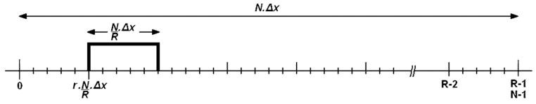
Diagram of rectangular window function of size N/R Δx to select a region at position r · N/R · Δx, which describes the dimension at the location of an STFT, whereas N is the number of pixels, R the number of regions for the STFT, and Δx is the pixel size. With this the complete Fourier transform can be considered as the sum of STFTs.

Equation [3] can be considered as the sum of STFT (25), i.e., Fourier transforms of data within the range specified by the rectangular window function at position $r·\frac{N}{R}·\mathrm{\Delta }x$:

$$S(k)=\sum _{r=0}^{R-1}\underset{S(k-k_{\mathit{sus}})}{\underbrace{\mathit{STF}{T}_{\gamma }\left(\rho (n·\mathrm{\Delta }x)·e^{-i·2\pi ·\gamma ·G_x^{\mathit{sus}}(\gamma )·TE·n·\mathrm{\Delta }x}\right)}},\mathit{with}{k}_{\mathit{sus}}(r)-\gamma ·G_{x^{\mathit{sus}}}(r)·TE$$ [4]

Therefore, the complete signal S(k) in k-space is the sum over locally shifted STFT, where the shift k_sus is given by the local susceptibility gradient. Due to the short length and position of the rectangular window function, the shape of the STFT is changed by a convolution with a sinc-function and phase term. However, it is important to note that the convolution does not alter the position of the maximum. Hence the local susceptibility gradient for each region can be determined from the position of the maximum in the local “short term” k-space. For example, the local susceptibility gradient in the region r can be determined by performing a STFT over pixel values of this region in image space and determining the position of the maximum in the “short term” k-space.

The echo-shift approach can be extended to a 2D and 3D data acquisition where the echo shift can occur in all three-dimensions. The susceptibility gradient G^sus for a given voxel is proportional to the shift in “short term” k-space m_x,y,z:

$$G_{x,y,z}^{\mathit{sus}}\approx -\frac{m_{x,y,z}·G_{x,y,z}^{\mathit{imaging}}·{\tau }_{x,y,z}}{m{\tau }_{x,y,z}+TE}.$$ [5]

Figure 2 shows the echo-shift in two dimensions. It depicts a simplified view on image-space and “short term” k-space for two different regions. The arrows in the different regions in image space symbolize voxels that are affected by susceptibility gradients in the direction of the arrow. The vector components can be determined from the position of the maximum in “short term” k-space of the different regions. For example the susceptibility gradient in region A points in the negative x-direction (arrow A in Fig. 2). This gradient can be determined from the position of the maximum in the “short term” k-space, which is shifted along the negative x-direction. A susceptibility gradient that has an x and y component (arrow B in Fig. 2) shifts the in the x and y component of the “short term” k-space. As described above, the global k-space can be determined by the sum over all “short term” k-space data.

FIG. 2.

Exemplified visualization of the echo shift in “short-term” k-space (right) that is induced by susceptibility gradients indicated in the image-space grid (left). These are indicated by arrows in the image-space pointing in the direction of the susceptibility gradient. By fitting, e.g., a Lorentzian-shaped curve to the data, the position of the maximum can be determined in the low-resolution “short-term” k-space. By repeating this procedure also in the z-direction, a susceptibility gradient vector is generated. [Color figure can be viewed in the online issue, which is available at www.interscience.wiley.com.]

If there is no B₀ inhomogeneity in a large portion of the object and only a small susceptibility gradient is present in one region, it would be difficult to determine this small echo-shift from the global k-space, since the shifted echo will be overlapped by the main echo in the center of the global k-space. In contrast to this, the echo shift can be determined from the “short term” k-space of this region, since it contains only the local information. In order to determine small echo shifts in the “short term” k-space, which has low-resolution, fitting of the “short term” k-space data can be applied. Furthermore, it is possible to discriminate echoes with a similar shift in the global k-space that are caused by susceptibility gradients in different regions. However, such shifted echoes can be determined by the local STFT, which are performed in different parts of image space separately.

MATERIALS AND METHODS

Calculation of Positive Contrast Images

The calculation of m_x,y,z was performed by using a 3D gradient echo dataset (see MR Experiments). For every voxel, a 1D STFT was performed subsequently in all spatial dimensions by taking into account the two adjacent voxels. This leads to a “short term” k-space consisting of only N = 3 Fourier components (k₋₁, k₀, k₊₁). Note that determination of the position of the maximum is only possible if the shift of the maximum away from k₀ is small. Therefore, if the echo shift was large enough to make the k₋₁ or k₊₁ component larger than k₀, the STFT was performed again over N = N + 1 voxels. This procedure was repeated, until a consistent determination of location of the maximum was possible. This hierarchical approach guarantees that only the minimum number of voxels is used for the Fourier transform, minimizing partial volume effects while enabling a stable fit in the determination of the echo shift. The procedure of enlarging the number of Fourier components depending on strength of the echo shift also guarantees an optimal spatial resolution, since the minimum number of voxels is used for the calculation of the susceptibility gradient vector. The optimal fitting procedure fits a sinc to the k-space data, but for this procedure a higher number of data points would be necessary. Since the k-space is coarsely resolved, the sinc-feature of the echo does not play a major role for the determination of the echo shift. For the determination of the echo shift only the main lobe of the sinc was fitted by using a quadratic fit.

By performing this 1D STFT separately in all spatial dimensions, all components of m_x,y,z can be determined for each voxel. This can be applied to all imaging voxels by means of a sliding window approach.

The magnitude of the vector m_x,y,z is proportional to the strength of the susceptibility gradient (see Eq. [5]). Plotting a parameter map of the magnitude of m_x,y,z generates an image that positively highlights the areas of strong changes in susceptibly, as it is known from positive contrast images shown in (17,19,20). This parameter map is called a positive contrast image throughout the rest of this work. The direction of the vector can also be employed to determine the heterogeneity of the source of the susceptibility gradient.

MR Experiments

Phantom experiments were performed on a 1.5T whole-body scanner (Achieva; Philips Medical Systems, Best, the Netherlands). A cylindrical glass bowl, diameter = 15 cm, filled with 6% gelatin was used. Care was taken to avoid the formation of air bubbles. The gelatin phantom contained four holes that were filled with either diluted SPIO (SHU 555 A, Resovist^®; Schering AG, Berlin, Germany) or agarose gel (8%). No glass or plastic tubes were used to avoid their additional susceptibility influence. Different concentrations of SPIOs were used to fill hole numbers 1 and 2 (0.65 μmol Fe/ml) and 4 (0.45 μmol Fe/ml), while hole number 3 was filled with 5% agarose gel. Complex data of a 3D gradient echo image were acquired by using a transmit/receive head coil: repetition time (TR) = 43 ms, echo time (TE) = 8 ms, flip angle = 30°, field of view (FOV) = 180 × 180 × 24 mm³, matrix size = 256 × 256 × 24, and number of averages = 4.

A second phantom experiment was carried out by placing an air-filled glass cylinder, diameter = 2.8 cm, perpendicular with respect to B₀, into a water-filled bowl. By choosing an equivalent model of an air-filled cylinder in a water bath and using the known susceptibilities of air and water, an accurate and reliable quantification of the measured susceptibility gradient was performed. Thereby the influence of the air cylinder on the magnetic field can be theoretically quantified and compared with the measured data as shown in the results section. 3D gradient echo imaging was performed by using a transmit/receive head coil: TR = 12.5 ms, TE = 10 ms, flip angle = 30°, FOV = 180 × 180 × 48 mm³, matrix size = 256 × 256 × 24, and number of averages = 1.

In vivo experiments were performed on nude rats on a 3T whole-body scanner (Intera; Philips Medical Systems) using a dedicated 7-cm-diameter rat solenoid RF coil (Philips Research Laboratories, Hamburg, Germany). All animal experiments were performed according to a protocol approved by the Clinical Center Animal Care and Use Committee at National Institutes of Health (NIH). For all studies, C6 glioma cells (ATCC, VA) were labeled with ferumoxides (Berlex Laboratories, NJ, USA) and protamine sulfate (FEPro) complexes using procedures previously described (26). The 5 × 10⁵ FEPro-labeled C6 glioma cells and nonlabeled control cells were implanted subcutaneously bilaterally in the flanks of six female nude rats (Harlen Sprague Dawley nu/nu). Animals were anesthetized with 1.5% to 2% isoflurane by a nosecone, and the heart rate and respirations were monitored with a pulse oximeter (MedRad LLC, Chicago, IL, USA) during the scan. 3D gradient echo imaging was performed with: TR = 16 ms, flip angle = 20°, matrix size = 256 × 256 × 32, FOV = 70 × 70 × 30 mm³, and number of averages = 4. The tumors were imaged 7 d after implantation of the cells as well as 14 d after implantation.

At water–fat boundaries, a phase shift in image space occurs that after FFT also is detected as an echo shift. These were suppressed by choosing in-phase echo time of TE = 4.8 ms for water and fat, which eliminates the phase shift.

All rats were euthanized after MRI and tumors were removed and fixed in 4% paraformaldehyde. Tumor sectioning for histological analysis was performed on 6-μm-thick slices. Tissue sections from the center of the tumor were stained with Prussian blue to evaluate the distribution of SPIO-labeled cells and counterstained with nuclear fast red as shown.

RESULTS

Phantom Study

A parametric map of the magnitude of the susceptibility gradient vector of the gelatin embedded with SPIOs is shown in Fig. 3. The gradient echo image allows no discrimination between the SPIO-filled holes and the agarose gel (Fig. 3a). By using the complex gradient echo dataset for the calculation of a susceptibility gradient map, the influence of the SPIO-filled holes can be differentiated from the agarose-filled hole (Fig. 3b). The brightness of the magnitude image of the susceptibility gradient map reflects the difference in SPIO concentration. Large-scale susceptibility influences at the border of the gelatin phantom appear to have lower signal intensity, since the susceptibility gradient per voxel is smaller than the gradient in the vicinity of the SPIO-filled holes. Figure 3 also demonstrates the selective nature of the method, since the agarose-filled hole is not visible on the susceptibility gradient map, because there is basically no difference in susceptibility between gelatin and agarose gel. Since the agarose shortens the T₂ due to its higher protein content, it appears hypointense or dark on the gradient echo image, but can be distinguished from the SPIO-filled holes via the susceptibility gradient map without the need of an additional image acquisition. The contrast-to-noise ratio (CNR) was calculated for the SPIO-filled hole A shown in Fig. 3; therefore, the noise was calculated in a 20 × 20 voxel region of interest in the middle of the phantom. For the T₂*-weighted image a CNR of 21 was calculated, whereas the SGM image revealed a CNR of 161 in this example. Since the SGM image is the result of a postprocessing method the direct comparison is difficult and will be part of a further investigation.

FIG. 3.

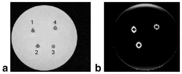
Gelatin phantom filled with different SPIO concentrations (1, 2, and 4) and agarose gel (3). a: The gradient echo image. b: A parametric map of the magnitude of the susceptibility gradient, that depicts positive contrast for the SPIO-filled holes and no contrast for the agarose. This allows a selective discrimination between SPIO and agarose, based on the induced susceptibility.

For the phantom measurement of the air filled cylinder a 3D susceptibility gradient map was calculated. Using this, a quantitative comparison can be made between a calculated susceptibility gradient and the measured susceptibility gradient by means of SGM: the in-plane field distribution f that is induced by a vertically positioned cylinder of radius a, can be described by the following analytical expression (27):

$$\mathrm{\Delta }f(r,\phi )=\frac{\mathrm{\Delta }\chi }{2}·\frac{a^2}{r^2}·cos(2\phi )·B_0,$$ [2]

where Δχ is the susceptibility difference between the cylinder and surroundings, r is the distance from the cylinder center, and φ is the angle relative to the main field, B₀. To simplify matters, we only look at one line of voxels with φ = 0, i.e., into the direction of B₀. The induced susceptibility gradient is then calculated by the first derivative with respect to r:

$$\frac{\partial \mathrm{\Delta }f(r)}{\partial r}=-\mathrm{\Delta }\chi ·\frac{a^2}{r^3}·B_0.$$ [3]

In a first-order approximation we ignored the influence of the glass walls and used the susceptibility difference of air/water Δχ = 9.04 × 10⁻⁶ (SI units) to calculate the susceptibility gradient as it is plotted in Fig. 4 (filled squares). The calculated echo shift was converted into a susceptibility gradient by means of Eq. [5]. The filled circles show the result of the SGM-derived results. An agreement of both curves can be observed with a root mean square error between the theoretical data and the measured susceptibility gradient of 0.093 mT/m.

FIG. 4.

Strength of the susceptibility gradient in the y-direction (parallel to B₀). Solid squares, calculated from known susceptibility changes induced by an air-filled cylinder. Solid circles: Measured susceptibility gradient.

In Vivo Study

Figure 5 illustrates a 4× photomicrograph of a tissue slice from an SPIO-labeled tumor, 2 weeks after implantation. The blue spots on the slice depict SPIO nanoparticles and correspond to the hypointense regions on the T₂*-weighted images (see Fig. 7a). The 20× photomicrograph indicates an inhomogeneous distribution of SPIO-labeled cells after 2 weeks.

FIG. 5.

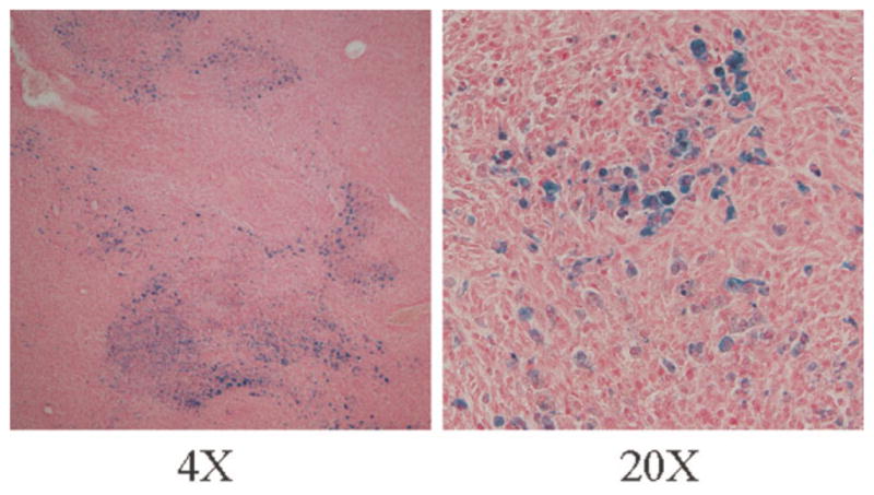
Histological verification of distribution of labeled cells inside the tumor, performed on 6-μm-thick slices. Tissue sections were stained with Prussian blue to evaluate the distribution of SPIO-labeled cells and counterstained with nuclear fast red.

FIG. 7.

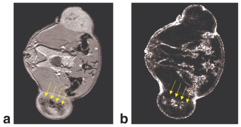
a: Two weeks after implantation the tumor has grown and the labeled tumor cells have been diluted, as can be seen in gradient echo image. b: The corresponding positive contrast image shows that the labeled cells can be imaged selectively, and that the non-labeled tumor shows no positive contrast. [Color figure can be viewed in the online issue, which is available at http://www.interscience.wiley.com.]

Figures 6 and 7 demonstrate the application of the SGM technique to in vivo cell tracking. Figure 6a depicts the gradient echo image of a SPIO-labeled C6 glioma flank tumor 1 week after implantation. Due to the small tumor size, the local iron concentration is high, and the tumor appears as hypointense region in the flank of the animal. Large susceptibility gradients arise at the interface between the iron-labeled tumor and the surrounding tissue, as shown in the positive contrast image in Fig. 6b. In this stage of the tumor growth, the labeled cells are still densely packed and influence the magnetic field on a scale much larger than cell dimensions, ranging over several voxels. Hence, the tissue containing the labeled cells can be treated like a large-scale magnetic dipole that exhibits strong susceptibility gradients at its border. The low signal intensities found within the tumor have two causes. First, the highly concentrated iron oxide–labeled cells are distributed homogeneously in the tumor. This homogeneous distribution of highly labeled cells leads to strong gradients at the border of the tumor, but to a homogeneous field offset inside the tumor. Therefore, no susceptibility gradients are observed inside the tumor. Second, the high iron concentration leads to signal voids in the gradient echo image, and as a result no SGM is possible for some voxels inside the tumor as there is simply no image information.

FIG. 6.

a: Gradient echo image of the tumor 1 week after implantation. Due to the small tumor size, the local iron concentration is rather high. b: Large susceptibility gradients arise at the interface between the iron-labeled tumor and the surrounding tissue as shown in the positive contrast image. [Color figure can be viewed in the online issue, which is available at http://www.interscience.wiley.com.]

Two weeks after implantation, the tumor is larger, and the SPIO nanoparticles in the tumor cells have been diluted with each cell division, resulting in isointense signal intensity in parts of the tumor on MRI (Fig. 7a). The heterogeneous cell distribution could also be verified via histology (Fig. 5). The corresponding positive contrast image shows that the labeled cells can be imaged selectively (Fig 7b) and that the nonlabeled tumor shows no positive contrast. Unlike the high iron oxide concentration shown in Fig. 6, no signal voids are observable here, the labeled cell distribution is heterogeneous and this is reflected in the pattern of the susceptibility gradients in the SGM map. The main fraction of the water-fat transitions has been suppressed by the in-phase echo time. Other susceptibility influences at the surface of the animal or close to the intestine cannot be suppressed and also give rise to a positive contrast as can be seen in Fig. 7b.

DISCUSSION

The major findings of this study show that the proposed SGM method is capable of producing positive contrast images that selectively highlight areas of changing susceptibility and detect the presence of SPIO-labeled cells in tissues. The main feature of the approach is that it calculates the absolute values of the echo shift from regular 3D gradient echo image datasets by means of 1D FFT, which requires no dedicated MRI sequences. This is advantageous over the detection of a linear phase change in the image domain, since no error-prone unwrapping procedures have to be performed, especially in three dimensions.

Performing the SGM postprocessing on the gradient echo image data allows for a specific discrimination between susceptibility-induced signal voids and other sources of signal voids. This opens up the possibility of discriminating, e.g., iron oxide–filled samples from agarose-filled samples, as shown in the phantom experiment. In the phantom experiment a higher CNR was also found for the SGM-derived positive contrast in comparison with the T₂*-weighted image, but this might not always be the case depending on signal to noise behavior in the image and the postprocessed SGM image. A comparison of sensitivities will be the topic of further investigation. This work shows that the method can be used to selectively discriminate susceptibility-induced signal voids, e.g., as arise from labeled cells, from other sources of signal voids, or from regions with short T₂ values. Positive contrast images can be used for additional information about susceptibly gradients; and since they are calculated from the T₂*-weighted images, they can be generated along with the T₂*-weighted images at no added cost in measurement time.

The absolute values of the susceptibility gradient vector can be assessed from the calculated echo shift via Eq. [2]. The magnitude of these vectors is visualized in a parameter map that represents a positive contrast image and allows for the discrimination of small and large susceptibility gradients via appropriate scaling.

The phantom experiments demonstrate that the absolute values of the susceptibility gradient agree with the theoretical predictions. The deviations from theory are induced by noise variations in the image. The upper limit of this method is reached if the susceptibility gradient induced echo shift is larger than the acquired k-space, shifting the echo peak out of k-space and leading to a signal void of the affected voxel. The method only takes into account the linear part of the susceptibility gradient; therefore, areas that exhibit also strong nonlinear contributions will be mapped with a lower accuracy. Since the nonlinearity will only be observed if a larger number of voxels is taken into account for the STFT, the treatment of nonlinear components would lower the resolution of the resulting susceptibility gradient map and was therefore not taken into account in this work.

The phantom experiments also demonstrate that the changes in susceptibility in all spatial dimensions can be taken into account by the SGM approach. The technique permits the retrospective generation of parametric maps that only utilize one or two spatial components for the generation of the positive contrast image. Using only one or two spatial components may be helpful if the other spatial components are strongly influenced by large-scale susceptibility artifacts that lead to a suppression or lack of visualization of small structures. On the other hand, it is also possible to use 2D gradient echo images to calculate positive contrast images, which will of course only show the susceptibility gradients in two dimensions.

Due to the fact that the susceptibility gradient is calculated by taking into account a n voxels for the STFT, positive contrast image resolution is affected by the value of n. Since the SGM method is performed via a sliding window approach, the loss in resolution compared to the original image is smaller than n, but a lower resolution of the SGM image will be observed compared to the original T₂*-weighted image.

Partial volume effects arise, if the susceptibility gradient extends for fewer than n voxels. A positive contrast in the susceptibility gradient magnitude map is still observed, but with a diminished absolute value. The fact that n voxels is needed for the calculation causes an averaging over these voxels in the determination of the susceptibility gradient. This leads to a partial volume effect since large variations within the group of n voxels that undergo STFT is not observable in the “shot term” k-space.

To reduce positive contrast artifacts arising from phase changes occurring at water-fat boundaries the echo time must be chosen to be in-phase. If this limits the desired application, a fat suppression pulse can also be used, which will be investigated in further studies.

Application of the SGM method in the flank tumor model demonstrated the first application of the technique to an in vivo setting. It gives a first impression of the sensitivity and selectivity as well as some of the limitations of this approach to detect the SPIO-labeled cells. When the concentration of iron in cells is high, a strong susceptibility gradient exists at the border of the tumor. The round shape of the positive contrast high signal intensity region circumferentially around the tumor shows the sensitivity of the SGM method in three-dimensions as can be seen in Fig. 6. The influence of all spatial directions is taken into account, leading to a ring-shaped positive contrast around the tumor. These results are similar to what was observed in the phantom study.

The positive contrast calculation of the 1-week-old tumor revealed that a cluster of 5 × 10⁶ million cells distributed over the small tumor induces macroscopic susceptibility gradients that can be similarly treated, such as the SPIO-filled holes in shown in Fig. 3. If the tumor grows, the cells start diluting. Since the SGM method detects changes in the susceptibility between voxels, the influence of the cells needs to spread over more than one imaging voxel. As can be seen in Fig. 7, the more heterogeneous cell distribution can still be imaged by means of SGM. Very small concentrations that only cause intravoxel dephasing and generate no changes in the magnetic field between voxels will be difficult to detect by means of the SGM method. Furthermore, the sensitivity of the SGM method compared to T₂*-weighted imaging of low-concentration SPIOs depends on several factors. For example, if the T₂* relaxation time of the surrounding tissue is long (e.g., on the order of 40 ms in brain), then the hypointense regions produced by labeled cells can be sensitively detected via a T₂*-weighted image. However, if the background T₂* of the tissue is relatively shorter, or if there is a strong heterogeneity in T₂ and T₂* within the region of interest, it will be more difficult to distinguish labeled cells within the tissue such as liver. In tissues with short or heterogeneous T₂ or T₂*, the SGM image will be a good complement to the T₂*-weighted image since it selectively depicts the SPIO-labeled cells; the image contrast is not dependent on differences in relaxation times, but on differences in susceptibility.

The generation of SGM maps does not require any specific imaging sequences other than the use of a gradient echo acquisition with an in-phase echo time. This is one advantage over previous positive-contrast techniques. The application of specific positive-contrast sequences has the advantage of providing the full spatial resolution and showing less partial volume effects at the cost of a longer measurement time (17,19,20). The approach of selectively saturating or exciting frequency shifted spins as shown in Refs. 19 and 20 gives rise to a different kind of positive contrast. These techniques will show all frequency-shifted areas including areas of homogeneous SPIO distribution, but they require an a priori estimate of the strength of the frequency shift. The SGM-generated positive contrast shows changes in susceptibility, meaning that areas of homogeneous SPIO distribution will show positive contrast at the border of the region. This is also a difference to the SWI method (24). SWI enhances the hypointensity in areas were the phase shows an offset, whereas the SGM method generates hyperintensity in areas of changing phases; i.e., strong susceptibility gradients. SWI therefore directly enhances phase-induced effects; SGM is sensitive to the first derivative of the phase. These two methods therefore generate somewhat complementary image information.

The methods described (21,22) also permit the selective highlighting of areas with large susceptibility gradients without the need of dedicated MR sequences. Whereas the calculation of the susceptibility influence is performed globally in k-space, the SGM approach deals with the data in image space. By performing localized 1D-STFT only the locally present susceptibility gradients will be observed in the “short term” k-space generated by means of STFT. Other—possibly stronger—susceptibility gradients stemming from a different spatial region will not interfere.

Apart from tracking of SPIO-labeled cells, the SGM technique may be useful in a wide range of applications. The method could be beneficial for the sensitive detection of iron oxide–based contrast agents in applications like lymph node detection, angiography, and inflammatory processes. Since the method can detect and quantify differences in the local susceptibility, it might also be used to highlight venous from arterial blood or reveal microhemorrhages or calcification within tissue. Furthermore, the positive contrast images derived from SGM can be used for a better visualization of devices such as stents, needles, or catheters without the need for an additional image acquisition.

CONCLUSIONS

We have proposed a new method for mapping of the susceptibility gradient vector from the complex data of gradient echo MR acquisitions. The susceptibility gradient map was used to quantify the susceptibility changes originated from an air-filled cylinder in a phantom. Furthermore, a positive contrast image was derived from a susceptibility gradient map to detect field inhomogeneity-inducing materials like SPIO-based contrast agents. The feasibility of SGM for in vivo detection of labeled cells was demonstrated in an animal model. The postprocessing method introduced extracts additional information from a T₂*-weighted image without the need of an extra measurement. The provided susceptibility gradient map exhibits a lower resolution than the original T₂*-weighted image, but the main feature is that it can be used to discriminate hypointensities induced by susceptibility gradients from other causes of hypointensity, e.g., to enlarge specificity of cell tracking in combination with the T₂*-weighted image. The method has a great potential to detect the susceptibility induced by contrast agents or medical devices in a wide range of applications.

References

- 1.Ogawa S, Menon RS, Tank DW, Kim SG, Merkle H, Ellermann JM, Ugurbil K. Functional brain mapping by blood oxygenation level dependent contrast magnetic resonance imaging. A comparison of signal characteristics with a biophysical model. Biophys J. 1993;64:803– 812. doi: 10.1016/S0006-3495(93)81441-3. [DOI] [PMC free article] [PubMed] [Google Scholar]
- 2.An H, Lin W. Cerebral oxygen extraction fraction and cerebral venous blood volume measurements using MRI: effects of magnetic field variation. Magn Reson Med. 2002;47:958–966. doi: 10.1002/mrm.10148. [DOI] [PubMed] [Google Scholar]
- 3.Rubin DL, Ratner AV, Young SW. Magnetic susceptibility effects and their application in the development of new ferromagnetic catheters for magnetic resonance imaging. Invest Radiol. 1990;25:1325–1332. doi: 10.1097/00004424-199012000-00010. [DOI] [PubMed] [Google Scholar]
- 4.Bakker CJ, Hoogeven RM, Weber J, van Vaals JJ, Viergever MA, Mali WP. Visualization of dedicated catheters using fast scanning techniques with potential for MR-guided vascular interventions. Magn Reson Med. 1996;36:816– 820. doi: 10.1002/mrm.1910360603. [DOI] [PubMed] [Google Scholar]
- 5.Ordidge RJ, Gorell JM, Deniau JC, Knight RA, Helpern JA. Assessment of relative brain iron concentrations using T2-weighted and T*2-weighted MRI at 3 Tesla. Magn Reson Med. 1994;32:335–341. doi: 10.1002/mrm.1910320309. [DOI] [PubMed] [Google Scholar]
- 6.Gandon Y, Guyader D, Heautot JF, Reda MI, Yaouanq J, Buhe T, Brissot P, Carsin M, Deugnier Y. Hemochromatosis: diagnosis and quantification of liver iron with gradient-echo MR imaging. Radiology. 1994;193:533–538. doi: 10.1148/radiology.193.2.7972774. [DOI] [PubMed] [Google Scholar]
- 7.Saini S, Stark DD, Hahn PF, Wittenberg J, Brady TJ, Ferrucci JT., Jr Ferrite particles: a superparamagnetic MR contrast agent for the reticuloendothelial system. Radiology. 1987;162:211–216. doi: 10.1148/radiology.162.1.3786765. [DOI] [PubMed] [Google Scholar]
- 8.Weissleder R, Elizondo G, Wittenberg J, Lee AS, Josephson L, Brady TJ. Ultrasmall superparamagnetic iron oxide: an intravenous contrast agent for assessing lymph nodes with MR imaging. Radiology. 1990;175:494– 498. doi: 10.1148/radiology.175.2.2326475. [DOI] [PubMed] [Google Scholar]
- 9.McLachlan SJ, Koutcher JA, Castellino RA. AMI-227-enhanced MR lymphography: usefulness for differentiating reactive from tumor-bearing lymph nodes. Radiology. 1994;193:501–506. doi: 10.1148/radiology.193.2.7972768. [DOI] [PubMed] [Google Scholar]
- 10.Anzai Y, Prince MR, Chenevert TL, Maki JH, Londy F, London M, McLachlan SJ. MR angiography with an ultrasmall superparamagnetic iron oxide blood pool agent. J Magn Reson Imaging. 1997;7:209–214. doi: 10.1002/jmri.1880070132. [DOI] [PubMed] [Google Scholar]
- 11.Weissleder R, Cheng HC, Bogdanova A, Bogdanov A., Jr Magnetically labeled cells can be detected by MR imaging. J Magn Reson Imaging. 1997;7:258–263. doi: 10.1002/jmri.1880070140. [DOI] [PubMed] [Google Scholar]
- 12.Bulte JW, Zhang S, van Gelderen P, Herynek V, Jordan EK, Duncan ID, Frank JA. Neurotransplantation of magnetically labeled oligodendrocyte progenitors: magnetic resonance tracking of cell migration and myelination. Proc Natl Acad Sci USA. 1999;96:15256–15261. doi: 10.1073/pnas.96.26.15256. [DOI] [PMC free article] [PubMed] [Google Scholar]
- 13.Bowen CV, Zhang X, Saab G, Gareau PJ, Rutt BK. Application of the static dephasing regime theory to superparamagnetic iron-oxide loaded cells. Magn Reson Med. 2002;48:52– 61. doi: 10.1002/mrm.10192. [DOI] [PubMed] [Google Scholar]
- 14.Ruehm SG, Corot C, Vogt P, Kolb S, Debatin JF. Magnetic resonance imaging of atherosclerotic plaque with ultrasmall superparamagnetic particles of iron oxide in hyperlipidemic rabbits. Circulation. 2001;103:415– 422. doi: 10.1161/01.cir.103.3.415. [DOI] [PubMed] [Google Scholar]
- 15.Schmitz SA, Taupitz M, Wagner S, Wolf KJ, Beyersdorff D, Hamm B. Magnetic resonance imaging of atherosclerotic plaques using super-paramagnetic iron oxide particles. J Magn Reson Imaging. 2001;14:355–361. doi: 10.1002/jmri.1194. [DOI] [PubMed] [Google Scholar]
- 16.Corot C, Petry KG, Trivedi R, Saleh A, Jonkmanns C, Le Bas JF, Blezer E, Rausch M, Brochet B, Foster-Gareau P, Baleriaux D, Gaillard S, Dousset V. Macrophage imaging in central nervous system and in carotid atherosclerotic plaque using ultrasmall superparamagnetic iron oxide in magnetic resonance imaging. Invest Radiol. 2004;39:619– 625. doi: 10.1097/01.rli.0000135980.08491.33. [DOI] [PubMed] [Google Scholar]
- 17.Seppenwoolde JH, Viergever MA, Bakker CJ. Passive tracking exploiting local signal conservation: the white marker phenomenon. Magn Reson Med. 2003;50:784–790. doi: 10.1002/mrm.10574. [DOI] [PubMed] [Google Scholar]
- 18.Frahm J, Merboldt KD, Hanicke W. Direct FLASH MR imaging of magnetic field inhomogeneities by gradient compensation. Magn Reson Med. 1988;6:474– 480. doi: 10.1002/mrm.1910060412. [DOI] [PubMed] [Google Scholar]
- 19.Cunningham CH, Arai T, Yang PC, McConnell MV, Pauly JM, Conolly SM. Positive contrast magnetic resonance imaging of cells labeled with magnetic nanoparticles. Magn Reson Med. 2005;53:999–1005. doi: 10.1002/mrm.20477. [DOI] [PubMed] [Google Scholar]
- 20.Stuber M, Gildon WD, Schaer M, Bulte JW, Kraitchman DL. Shedding light on the dark spot with IRON—a method that generates positive contrast in the presence of superparamagnetic nanoparticles. Proceedings of the 13th Annual Meeting of ISMRM; Miami Beach, FL, USA. 2005. [Google Scholar]
- 21.Posse S. Direct imaging of magnetic field gradients by group spin-echo selection. Magn Reson Med. 1992;25:12–29. doi: 10.1002/mrm.1910250103. [DOI] [PubMed] [Google Scholar]
- 22.Bakker CJ, Seppenwoolde JH, Vincken KL. Dephased MRI. Magn Reson Med. 2006;55:92–97. doi: 10.1002/mrm.20733. [DOI] [PubMed] [Google Scholar]
- 23.Reichenbach JR, Venkatesan R, Yablonskiy DA, Thompson MR, Lai S, Haacke EM. Theory and application of static field inhomogeneity effects in gradient-echo imaging. J Magn Reson Imaging. 1997;7:266–279. doi: 10.1002/jmri.1880070203. [DOI] [PubMed] [Google Scholar]
- 24.Haacke EM, Xu Y, Cheng YC, Reichenbach JR. Susceptibility weighted imaging (SWI) Magn Reson Med. 2004;52:612– 628. doi: 10.1002/mrm.20198. [DOI] [PubMed] [Google Scholar]
- 25.Allen JB, Rabiner LR. A unified approach to short-time Fourier analysis and synthesis. Proc IEEE. 1977;65:1558–1564. [Google Scholar]
- 26.Arbab AS, Yocum GT, Kalish H, Jordan EK, Anderson SA, Khakoo AY, Read EJ, Frank JA. Efficient magnetic cell labeling with protamine sulfate complexed to ferumoxides for cellular MRI. Blood. 2004;104:1217–1223. doi: 10.1182/blood-2004-02-0655. [DOI] [PubMed] [Google Scholar]
- 27.Haacke EM, Brown RW, Thompson MR, Venkatesan R. Magnetic resonance imaging: physical principles and sequence design. New York: Wiley-Liss; 1999. [Google Scholar]