Conductivity and permittivity imaging at 3.0T

Abstract

Tissue conductivity and permittivity are critical to understanding local radio frequency (RF) power deposition during magnetic resonance imaging (MRI). These electrical properties are also important in treatment planning of RF thermotherapy methods (e.g. RF hyperthermia). The electrical properties may also have diagnostic value as malignant tissues have been reported to have higher conductivity and higher relative permittivity than surrounding healthy tissue.

In this study, we consider imaging conductivity and permittivity using MRI transmit field maps (B₁⁺ maps) at 3.0 Tesla. We formulate efficient methods to calculate conductivity and relative permittivity from 2-dimensional B₁⁺ data and validate the methods with simulated B₁⁺ maps, generated at 128 MHz. Next we use the recently introduced Bloch-Siegert shift B₁⁺ mapping method to acquire B₁⁺ maps at 3.0 Tesla and demonstrate conductivity and relative permittivity images that successfully identify contrast in electrical properties.

INTRODUCTION

The conductivity and permittivity of tissue are critical to understanding local radio frequency (RF) power deposition, also known as local specific absorption rate (local SAR) during magnetic resonance imaging. This local distribution of RF power has come under increasing study with higher field imaging and with the use of multiple transmitters, two trends that have resulted in a number of numerical studies to evaluate the potential for concentrated RF power deposition (i.e. local hot spots) in the body (1, 2).

Tissue electrical properties are also important in the therapeutic application of heat using radio frequency, for example, RF hyperthermia. During the application of RF power, the temperature rise at a given location in the body is proportional to the tissue conductivity and the square of the electric field strength at that location. The electric field strength and distribution in turn depends on the conductivity and permittivity values of the tissue. Therefore, tissue electrical properties are important parameters in hyperthermia treatment planning and optimization (3).

Tissue electrical parameters may also have diagnostic value as the conductivity and permittivity of malignant tissue have been reported to be higher than surrounding healthy tissue (4–6).

Therefore, a method that non-invasively estimates the conductivity and permittivity in a clinically acceptably time has multiple benefits, namely in evaluating RF safety, in RF therapeutic methods and potentially in diagnosing tissue abnormality.

In prior work, electrical impedance tomography has been applied to estimate tissue electrical properties (7). In this method, electrodes are placed on the surface of the body, currents applied by one set of electrodes, resulting voltages recorded by another set of electrodes and an inverse problem is solved to estimate the conductivity and permittivity of tissue within the body. However, in addition to the inconvenience of using electrodes, electrical impedance tomography leads to computational issues as the inverse problem is ill-posed.

In more recent work, estimation of tissue electrical properties using the spatial variation of transmit magnetic field in MRI (B₁⁺ maps) was studied in (8). However, the proposed method required, in addition to the transmit field (B₁⁺), the receiver sensitivity (B1⁻) and the z-component of the RF magnetic field (H_z), which are not typically available. In a following study, this method was extended to use only B₁⁺ data and an integral form for calculating electrical properties from B₁⁺ maps was presented (9). The gradient of the B₁⁺ is integrated over a closed volume to estimate the electrical properties with this approach.

An alternative approach is to use the second derivative of B₁⁺. In early work, equations for the conductivity and relative permittivity of a layered object were presented in terms of the second derivative of B₁⁺ in a layered model (10). This has been extended to arbitrary volume of constant electrical properties using second partial derivatives of B₁⁺ in x, y and z directions (Laplacian) in (11–14).

In this work, we formulate the Laplacian based calculation of conductivity and permittivity using central difference equations. This calculation can be carried out using B₁⁺ maps acquired in 2-dimensional slices. These equations are validated by estimating the conductivity and permittivity of a human head model using B₁⁺ maps generated from electromagnetic simulation at 128MHz, corresponding to 3.0T imaging. Next, the recently introduced Bloch-Siegert B₁⁺ mapping (15) technique is used to generate B₁⁺ maps at 3.0T and the algorithm is evaluated for a head phantom.

THEORY

In this section, a theoretical relationship between the spatial variation of B₁⁺, and conductivity and permittivity is given. Using the phasor notation for time harmonic fields, the circularly polarized, transmit magnetic field $B_1^{+}(\mathbf{x})$ at location x = (x, y, z) is given by,

$$B_1^{+}(\mathbf{x})=\frac{\mu }{2}\left(H_x(\mathbf{x})+{jH}_y(\mathbf{x})\right)$$ [1]

where μ is the permeability, H_x and H_y are the complex x and y components of the magnetic field (16). The spatial variation of B₁⁺ can be related to electrical properties starting with Ampere’s Law and Faraday’s Law and using the divergence equation (11). However, a concise derivation, using the Helmholtz equation is given here (13). In a source free region of constant electrical properties, the x and y components of the magnetic field satisfies (17)

$${\nabla }^2{H}_x(\mathbf{x})+{\omega }^2\mu \epsilon (\mathbf{x})\left(1+\frac{\sigma (\mathbf{x})}{j\omega \epsilon (\mathbf{x})}\right)H_x(\mathbf{x})=0$$ [2]

$${\nabla }^2{H}_y(\mathbf{x})+{\omega }^2\mu \epsilon (\mathbf{x})\left(1+\frac{\sigma (\mathbf{x})}{j\omega \epsilon (\mathbf{x})}\right)H_y(\mathbf{x})=0$$ [3]

Where ∇²( ) is the Laplace operator, ω is the frequency in radians/s, μ is the permeability, ε is the permittivity, (ε= ε_rε₀, where ε_r is the relative permittivity, ε₀=8.8542·10⁻¹² F/m is the free space permittivity), and σ is the conductivity. The permeability μ is assigned 4π·10⁻⁷ H/m to all tissue types. Then performing [2] + j[3], using the definition of B₁⁺ and recognizing the linearity of Laplace operator, we obtain

$${\nabla }^2{B}_1^{+}(\mathbf{x})+{\omega }^2\mu \epsilon (\mathbf{x})\left(1+\frac{\sigma (\mathbf{x})}{j\omega \epsilon (\mathbf{x})}\right)B_1^{+}(\mathbf{x})=0$$ [4]

Then by separating the real and imaginary components of the equation, we arrive at

$${\epsilon }_r(\mathbf{x})=\frac{-1}{{\omega }^2\mu {\epsilon }_0}Re\left\{\frac{{\nabla }^2{B}_1^{+}(\mathbf{x})}{B_1^{+}(\mathbf{x})}\right\}$$ [5]

$$\sigma (\mathbf{x})=\frac{1}{\omega \mu }Im\left\{\frac{{\nabla }^2{B}_1^{+}(\mathbf{x})}{B_1^{+}(\mathbf{x})}\right\}$$ [6]

Where the material properties of relative permittivity (ε_r) and conductivity (σ ) are given in terms of the transmit field B₁⁺.

METHODS

Central difference equations

To formulate equations for discrete data, expand equation [5]:

$${\epsilon }_r(\mathbf{x})=\frac{-1}{{\omega }^2\mu {\epsilon }_0}Re\left\{\frac{1}{B_1^{+}(\mathbf{x})}\left(\frac{{\partial }^2}{\partial x^2}{B}_1^{+}(\mathbf{x})+\frac{{\partial }^2}{\partial y^2}{B}_1^{+}(\mathbf{x})+\frac{{\partial }^2}{\partial z^2}{B}_1^{+}(\mathbf{x})\right)\right\}$$

Assuming that the volume of interest is discretized in steps of (Δx,Δy,Δz) such that the location x =(iΔx, jΔy, kΔz) can be represented as (i, j, k), partial second derivatives can be calculated as (18)

$$\begin{array}{l}\frac{{\partial }^2}{\partial x^2}{B}_1^{+}(\mathbf{x}):\frac{B_1^{+}(i+2,j,k)-2B_1^{+}(i,j,k)+B_1^{+}(i-2,j,k)}{4\mathrm{\Delta }{x}^2}\triangleq {\delta }_x(i,j,k)\\ \frac{{\partial }^2}{\partial y^2}{B}_1^{+}(\mathbf{x}):\frac{B_1^{+}(i,j+2,k)-2B_1^{+}(i,j,k)+B_1^{+}(i,j-2,k)}{4\mathrm{\Delta }{y}^2}\triangleq {\delta }_y(i,j,k)\\ \frac{{\partial }^2}{\partial z^2}{B}_1^{+}(\mathbf{x}):\frac{B_1^{+}(i,j,k+2)-2B_1^{+}(i,j,k)+B_1^{+}(i,j,k-2)}{4\mathrm{\Delta }{z}^2}\triangleq {\delta }_z(i,j,k)\end{array}$$

Then the permittivity is:

$${\widehat{\epsilon }}_r(i,j,k)=\frac{-1}{{\omega }^2\mu {\epsilon }_0}Re\left\{\frac{{\delta }_x(i,j,k)+{\delta }_y(i,j,k)+{\delta }_z(i,j,k)}{B_1^{+}(i,j,k)}\right\}$$ [7]

Similarly, the conductivity is

$$\widehat{\sigma }(i,j,k)=\frac{1}{\omega \mu }Im\left\{\frac{{\delta }_x(i,j,k)+{\delta }_y(i,j,k)+{\delta }_z(i,j,k)}{B_1^{+}(i,j,k)}\right\}$$ [8]

The equations show that to estimate relative permittivity and conductivity at location (i, j,k), we require B₁⁺ data at (i, j, k),(i ± 2, j,k),(i, j ± 2,k),(i, j, k ± 2) points, for a total of 7 data points(19). Note the equations use next to nearest neighbor points in the calculation and not the nearest neighbor points.

Estimation of relative permittivity from B₁⁺ magnitude and conductivity from B₁⁺ phase

Although the relative permittivity and conductivity are estimated using complex B₁⁺, relative permittivity is mostly dependent on the magnitude of B₁⁺ and therefore can be calculated using only B₁⁺ magnitude maps and the conductivity is mostly dependent on the phase of B₁⁺ and therefore can be calculated by using only B₁⁺ phase maps(9, 13).

For permittivity imaging with only B₁⁺ magnitude maps,

$${\epsilon }_r(\mathbf{x})\approx \frac{-1}{{\omega }^2\mu {\epsilon }_0}\left\{\frac{{\nabla }^2\left|B_1^{+}(\mathbf{x})\right|}{\left|B_1^{+}(\mathbf{x})\right|}\right\}$$ [9]

and therefore, the estimate can be carried out as

$${\widehat{\epsilon }}_r(i,j,k)\approx \frac{-1}{{\omega }^2\mu {\epsilon }_0}\left\{\frac{{\delta }_x(i,j,k)+{\delta }_y(i,j,k)+{\delta }_z(i,j,k)}{\left|B_1^{+}(i,j,k)\right|}\right\}$$ [10]

where the partial derivative terms δ_x (i, j, k),δ_y (i, j,k ) and δ_z (i, j, k) are also calculated using the magnitude of B₁⁺.

For conductivity imaging with only B₁⁺ phase maps, with the phase of B₁⁺ defined as

$$\begin{array}{c}\phi (\mathbf{x})\triangleq Ph(B{1}_1^{+}(\mathbf{x}))\\ \sigma (\mathbf{x})\approx \frac{1}{\omega \mu }Im\left\{\frac{1}{cos(\phi (\mathbf{x}))+j\ast sin(\phi (\mathbf{x}))}{\nabla }^2(cos(\phi (\mathbf{x}))+j\ast sin(\phi (\mathbf{x}))\right\}\end{array}$$ [11]

and therefore the estimate can be carried out as

$$\widehat{\sigma }(i,j,k)\approx \frac{1}{\omega \mu }Im\left\{\frac{1}{cos(\phi (i,j,k))+j\ast sin(\phi (i,j,k))}\left({\delta }_x(i,j,k)+{\delta }_y(i,j,k)+{\delta }_z(i,j,k)\right)\right\}$$ [12]

Here the partial derivatives δ_x (i, j, k),δ_y (i, j,k ) and δ_z (i, j, k) are also calculated using cos(φ(i, j, k)) + j *sin(φ(i, j, k))

Use of a skip factor in the calculation of Laplacian

Additive noise in B₁⁺ maps can corrupt the estimation of the Laplacian and therefore, the accuracy of electrical properties estimate. This issue can be addressed by evaluating the Laplacian over a larger volume. Define an integer skip factor (sf=1,2,3,..). Then the partial derivatives can be estimated as

$$\begin{array}{l}{\delta }_x(i,j,k)=\frac{B_1^{+}(i+2\ast sf,j,k)-2B_1^{+}(i,j,k)+B_1^{+}(i-2\ast sf,j,k)}{4{(sf\ast \mathrm{\Delta }x)}^2}\\ {\delta }_y(i,j,k)=\frac{B_1^{+}(i,j+2\ast sf,k)-2B_1^{+}(i,j,k)+B_1^{+}(i,j-2\ast sf,k)}{4{(sf\ast \mathrm{\Delta }y)}^2}\\ {\delta }_z(i,j,k)=\frac{B_1^{+}(i,j,k+2\ast sf)-2B_1^{+}(i,j,k)+B_1^{+}(i,j,k-2\ast sf)}{4{(sf\ast \mathrm{\Delta }z)}^2}\end{array}$$

As the skip factor increases, the numeric values of the difference terms increase relative to the noise, leading to better estimates.

Electromagnetic simulations

In order to verify the equations, B₁⁺ maps were generated from an electromagnetic simulation (HFSS, Ansoft Corp, Pittsburgh, PA, USA). A human head model was used in a birdcage type transmit coil(20) to obtain H_x and H_y in the axial planes. These were processed to find B₁⁺ using equation [1]. Then using equations [5] and [6], the relative permittivity and conductivity were estimated and compared with known electrical properties from the model.

The transmit coil model was a 16-rung, shielded birdcage coil, diameter 28cm, rung length 28cm and rung to shield spacing of 3.5cm. Each rung had a unit amplitude current source at the center of rung. The phases of the current sources were assigned a step increment from rung to rung, equal to 2π/16, to generate a circular polarized magnetic field. The frequency of each current source was 128MHz and the coil model simulated a low pass birdcage coil operating in a 3.0T imaging system.

The human head model had 5 components with each component representative of sections of the human head anatomy and assigned a tissue type with corresponding electrical properties. The components and the electrical properties were brain_frontal (εr=67.93, σ=0.54 S/m), cerebellum (εr=83.42, σ=0.82 S/m), eyes_left (εr=69.07, σ=1.51 S/m), eyes_right (εr=69.07, σ=1.51 S/m), and body_exterior (εr=64.7, σ=0.74 S/m). The model electrical properties resolution was 4mm in x, y, and z directions. The model and a cut-plane view of the central axial plane are shown in Fig. 1. This plane intersected the components brain_frontal and body_exterior.

Figure 1.

Human head model in birdcage coil (left), cut-plane view of the central axial plane (right)

Following the convergence of the finite element simulation in HFSS, the magnetic field quantities H_x and H_y were exported in a 24cm × 24cm axial plane region using a 128×128 sampling grid. This region and grid corresponded to a typical 128 × 128, 24cm field of view (FOV) MR image. In addition to the central axial slice, magnetic field data were exported for two slices at 5mm spacing in the superior direction (+z-direction) and two slices at 5mm spacing in the inferior direction (−z-direction), for a total of 5 slices.

The H_x and H_y data were imported to Matlab (Mathworks, Natick, MA, USA) and B₁⁺ maps were calculated for each slice using equation [1]. The relative permittivity and conductivity of the central axial slice were estimated using B₁⁺ data from the central axial slice, axial slice 10mm in the superior direction and axial slice 10mm in the inferior direction. The discretization steps in this case were Δx =1.875mm, Δy = 1.875mm, and Δz = 5mm. The equations [5] and [6] were then evaluated in Matlab. At each pixel, the calculation results were accepted based on prior knowledge, discarded otherwise. For example, the relative permittivity of tissue in the human body is typically in the range of 1 – 100, so results outside this range were discarded. Similarly, conductivity values outside the range of 0 – 4 S/m were discarded.

Phantom experiments

Next, a head phantom (Phantom Labs, Salem, NY, USA) was used in experimental validation of the method. The head phantom had two compartments; one inner, smaller compartment (20mm diameter, 35mm long) and an outer compartment. A photo of the phantom is shown in Fig. 2.

Figure 2.

Photo of the phantom. The outer compartment and inner compartment can be filled with different fluids

In the first experiment, the phantom was filled with non-conducting fluids, B₁⁺ magnitude data acquired using the recently introduced Bloch-Siegert shift B₁⁺ mapping method (15) and relative permittivity was estimated.

In the second experiment, the inner compartment was filled with a salt solution, B₁⁺ magnitude and phase data acquired and both relative permittivity and conductivity were estimated.

Head phantom – non-conducting fluids

The outer compartment of the head phantom was filled with 50% (volume) iso-propanol and 50% distilled water solution. The inner compartment was filled with distilled water. In order to reduce T1 relaxation time, copper sulphate was added to both solutions until concentration was 1g/liter of copper sulphate in the final prepared solution.

The relative permittivity based on literature is 18 for iso-propanol and 81 for distilled water (21). Using the dielectric mixture formula ((22), power law, β=1/2), we expected the 50% mixture in outer compartment to have a relative permittivity of 43.8.

The head phantom was placed in a 16 rung, quadrature transmit and receive head coil (Model 5182872 HDx, GE Healthcare, Waukesha, WI, USA). The phantom was aligned such that the central axial plane bisected the inner compartment of the phantom.

Then data for Bloch-Siegert shift based B₁⁺ mapping were acquired in a 3.0T scanner (Discovery MR 750, GE Healthcare, Waukesha, WI, USA) for three axial plane slices with the following parameters: FOV 24cm, slice thickness 5mm, spacing 5mm, resolution 128×128, TE 30ms, TR 800ms. At each slice, the B₁⁺ mapping pulse sequence generated two off resonance images (+/− 4 kHz) using 6ms long Fermi pulses to induce B₁⁺ dependent phase shifts in the images. From the two off resonance images, a phase difference image was calculated in Matlab, square root calculated and scaled to obtain the B₁⁺ map for each slice (15).

The B₁⁺ data were then used in the calculation of relative permittivity. At each pixel, the calculation results were accepted if within 1 – 100 range, discarded otherwise. The skip factors were used to improve the estimates. However, to estimate electrical properties using only the three axial plane B₁⁺ maps, the Laplacian was evaluated on a larger in plane area, rather than in a larger volume, by using skip factors in the calculation of x and y partial derivatives only.

The relative permittivity images were calculated for skip factors 1, 2 and 3 and the images were combined to obtain the final image. At any given pixel, an estimate from higher skip factor replaced an estimate from lower skip factor.

Head phantom – conducting fluids

In the next experiment, the inner compartment was filled with a salt solution (9 g/liter) and 1g/liter of copper sulphate. Data for Bloch-Siegert shift based B₁⁺ mapping were acquired for three axial plane slices with the following parameters: FOV 24cm, slice thickness 6mm, spacing 6mm, resolution 128×128, TE 30ms, TR 800ms.

In order to estimate conductivity, B₁⁺ phase, in addition to B₁⁺ magnitude is required. The phase of a spin echo image in a switched mode, quadrature birdcage coil has been shown to be approximately half of B₁⁺ phase (8, 13, 14). Under axial rotational and mirror symmetry, this relationship was shown to be exact (23).

Spin echo images were acquired for all three slices with the same alignment, but with TR 400ms. The phase encoding direction was A/P (anterior/posterior) in these images.

The spin echo images have a linear phase term and an additional constant phase, unrelated to phase variation due to the imaging sample properties. An efficient algorithm to remove the linear phase term using the autocorrelation of image pixels and the constant phase term using histogram analysis was presented in (24). This method was used to correct spin echo image phase.

The B₁⁺ magnitude and phase were combined to obtain complex B₁⁺, and conductivity and relative permittivity images were constructed. As in the previous section, skip factors 1, 2 and 3 were used in the calculation of x and y partial derivatives, and the three images from each skip factor were combined to obtain final conductivity and relative permittivity images.

RESULTS

Electromagnetic simulations

The magnitude and phase of simulated B₁⁺ for the central axial slice are shown in Fig. 2. The calculated electrical properties images for the central axial slice are shown in Fig. 3. The left hand figure shows the estimated conductivity and the right hand figure shows the estimated relative permittivity. A comparison of the model electrical properties and estimated electrical properties is given in Tables 1 and 2. The estimated values are in good agreement with model parameters.

Figure 3.

Simulation results: B1⁺ magnitude (left, μTesla) and phase (right, degrees) at central axial plane

TABLE 1.

Estimated values of Relative Permittivity

Component	Model	Estimated
		Mean	Std. dev.
brain_frontal	67.93	66	10
body_exterior	64.7	59.9	15

TABLE 2.

Estimated values of conductivity

Component	Model (S/m)	Estimated
		Mean (S/m)	Std. dev.
brain_frontal	0.54	0.57	0.16
body_exterior	0.74	0.75	0.245

Phantom experiments

Head phantom – non-conducting fluids

The B₁⁺ maps for the head phantom filled with 50% mixture of iso-propanol and distilled water (outer compartment) and distilled water (inner compartment) are shown in Fig. 5. The relative permittivity images calculated from these B₁⁺ maps are shown in Fig. 6. The images for each of the skip factor 1, 2, and 3 are shown and the images demonstrate the improvement as the skip factor is increased. The final relative permittivity image, after combining the images for each skip factor, is shown in Fig. 7. The image shows the lower relative permittivity of the outer compartment and the higher relative permittivity of the inner compartment of the head phantom.

Figure 5.

|B₁⁺| in central axial plane (center) and in axial planes +/− 10mm in S/I directions (right, left, units μTesla). The phantom inner compartment has distilled water and outer compartment has 50% mix of iso-propanol and water

Figure 6.

Permittivity image with Laplacian calculated over larger and larger areas (sf=1 (left), sf=2 (center), and sf=3 (right))

Figure 7.

Final relative permittivity image (left). The inner compartment has distilled water and the outer compartment has 50% mix of iso-propanol and water. The estimated values on a line that runs across the image, through the inner compartment, is shown on right

Head phantom – conducting fluids

The B₁⁺ maps for the head phantom filled with 50% mixture of iso-propanol and distilled water (outer compartment) and salt water (inner compartment) are shown in Fig. 8.

Figure 8.

|B₁⁺| in central axial plane (center) and in axial planes +/− 12mm in S/I directions (right, left, units μTesla). The phantom inner compartment has a salt solution and outer compartment has 50% mix of iso-propanol and water

The original spin echo image phase and the phase after removing the linear and constant phase terms are shown in Fig. 9.

Figure 9.

Spin echo phase for the three slices (top, degrees), after removing linear and constant phase terms (bottom, degrees). Note: The color scales are different in top and bottom images.

The calculated conductivity images for skip factor 1, 2, and 3 are shown in Fig. 10. The conductivity images incrementally improve as the skip factor increases. There is similar improvement in the permittivity images, but are not shown as they are similar to Fig. 6.

Figure 10.

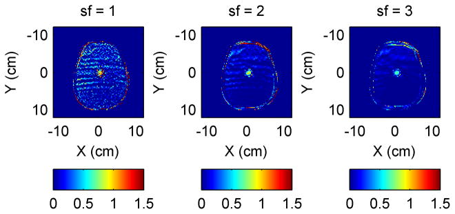
Conductivity images with Laplacian calculated over larger and larger areas (sf=1 (left), sf=2 (center) and sf=3 (right))

The final conductivity and relative permittivity images, after combining the images for skip factors 1, 2, and 3 are shown in Fig. 11. The images show the higher conductivity and the higher relative permittivity of the inner compartment.

Figure 11.

Conductivity image (left, S/m) and the permittivity image (right) for the central axial plane; inner compartment has a salt solution (distilled water with 9g/liter of salt) and outer compartment has 50% mix of iso-propanol and water

DISCUSSION AND CONCLUSION

The MRI B₁⁺ based electrical properties imaging offers a non-invasive and computationally efficient method as the B₁⁺ maps are obtained in non-invasive imaging routines and conductivity and relative permittivity images are calculated using difference equations.

Conductivity and relative permittivity estimated from simulated B₁⁺ maps showed good agreement with model electrical properties. The variance of the estimated values was highly correlated to the size of the hexahedral shaped mesh used in the finite element simulation. The variance decreased as the finite element mesh size was reduced. The results presented here were obtained by restricting the largest mesh element in the region of interest to be no larger than 5mm. This turned out to be an acceptable engineering compromise between the accuracy of electrical properties images and the required computer memory and the convergence time for the simulation.

The use of a skip factor in the calculation of Laplacian was an effective method to improve the estimates in the presence of noise in B₁⁺ maps, yet retained the computational efficiency of the calculation. In general, the electrical properties estimates improved as the skip factor was increased. However, when larger skip factors were used, poor estimates at material boundaries occurred. As invalid estimates were discarded, the image boundaries became smaller. The calculation of electrical properties images for skip factors 1, 2, 3 and combining the images turned out to be a good compromise between accuracy and image resolution as the phantom experiments successfully identified higher conductivity and higher relative permittivity in a localized region of 2cm × 3.5cm in an average head size volume.

The results point to the feasibility of imaging conductivity and relative permittivity in a non-invasive and computationally efficient manner using Bloch-Siegert shift based B₁⁺ mapping and central difference based equations.

Figure 4.

Conductivity image (left, S/m), and relative permittivity image (right) obtained from simulated B1⁺ data

References

- 1.Wang Z, Lin JC, Mao W, Liu W, Smith MB, Collins CM. SAR and temperature: Simulations and comparison to regulatory limits for MRI. Journal of Magnetic Resonance Imaging. 2007;26(2):437–41. doi: 10.1002/jmri.20977. [DOI] [PMC free article] [PubMed] [Google Scholar]
- 2.Yeo DTB, Wang Z, Loew W, Vogel MW, Hancu I. Local specific absorption rate in high-pass birdcage and transverse electromagnetic body coils for multiple human body models in clinical landmark positions at 3T. Journal of Magnetic Resonance Imaging. 2011;33(5):1209–17. doi: 10.1002/jmri.22544. [DOI] [PMC free article] [PubMed] [Google Scholar]
- 3.Das SK, Clegg ST, Samulski TV. Computational techniques for fast hyperthermia temperature optimization. AAPM. 1999:319–28. doi: 10.1118/1.598519. [DOI] [PubMed] [Google Scholar]
- 4.Fear EC, Hagness SC, Meaney PM, Okoniewski M, Stuchly MA. Enhancing breast tumor detection with near-field imaging. Microwave Magazine, IEEE. 2002;3(1):48–56. [Google Scholar]
- 5.Joines WT, Zhang Y, Li C, Jirtle RL. The measured electrical properties of normal and malignant human tissues from 50 to 900 MHz. Medical physics. 1994;21(4):547–50. doi: 10.1118/1.597312. [DOI] [PubMed] [Google Scholar]
- 6.Chaudhary SS, Mishra RK, Swarup A, Thomas JM. Dielectric properties of normal and malignant human breast tissue at radiowave and microwave frequencies. Indian Journal of Biochemistry and Biophysics. 1984;21:76–9. [PubMed] [Google Scholar]
- 7.Saulnier GJ, Blue RS, Newell JC, Isaacson D, Edic PM. Electrical impedance tomography. Signal Processing Magazine, IEEE. 2001;18(6):31–43. [Google Scholar]
- 8.Katscher U, Voigt T, Findeklee C, Vernickel P, Nehrke K, Dossel O. Determination of electric conductivity and local SAR via B1 mapping. IEEE transactions on medical imaging. 2009;28(9):1365–74. doi: 10.1109/TMI.2009.2015757. Epub 2009/04/17. [DOI] [PubMed] [Google Scholar]
- 9.Voigt T, Katscher U, Doessel O. Quantitative conductivity and permittivity imaging of the human brain using electric properties tomography. Magnetic resonance in medicine : official journal of the Society of Magnetic Resonance in Medicine/Society of Magnetic Resonance in Medicine. 2011;66(2):456–66. doi: 10.1002/mrm.22832. Epub 2011/07/21. [DOI] [PubMed] [Google Scholar]
- 10.Haacke EM, Petropoulos LS, Nilges EW, Wu DH. Extraction of conductivity and permittivity using magnetic resonance imaging. Physics in medicine and biology. 1991;36(6):723. [Google Scholar]
- 11.Bulumulla SB, Yeo TB, Zhu Y, editors. International Society for Magnetic Resonance in Medicine. Honolulu, Hawaii: 2009. Direct calculation of tissue electrical parameters from B1 maps. [Google Scholar]
- 12.Cloos MA, Bonmassar G, editors. International Society for Magnetic Resonance in Medicine. Honolulu, Hawaii: 2009. Towards direct B1 based local SAR estimation. [Google Scholar]
- 13.Wen H. Noninvasive quantitative mapping of conductivity and dielectric distributions using RF wave propagation effects in high-field MRI. journal article. 2003;5030(1):471–7. [Google Scholar]
- 14.van Lier AL, Brunner DO, Pruessmann KP, Klomp DW, Luijten PR, Lagendijk JJ, et al. B 1+ Phase mapping at 7 T and its application for in vivo electrical conductivity mapping. Magnetic resonance in medicine : official journal of the Society of Magnetic Resonance in Medicine/Society of Magnetic Resonance in Medicine. 2011 doi: 10.1002/mrm.22995. Epub 2011/06/29. [DOI] [PubMed] [Google Scholar]
- 15.Sacolick LI, Wiesinger F, Hancu I, Vogel MW. B1 mapping by Bloch-Siegert shift. Magnetic Resonance in Medicine. 2010;63(5):1315–22. doi: 10.1002/mrm.22357. [DOI] [PMC free article] [PubMed] [Google Scholar]
- 16.Hoult DI. The principle of reciprocity in signal strength calculations—A mathematical guide. Concepts in Magnetic Resonance. 2000;12(4):173–87. doi: 10.1002/1099-0534(2000)12:4<173::aid-cmr1>3.0.co;2-q. [DOI] [Google Scholar]
- 17.Cheng DK. Fundamentals of Engineering Electromagnetics. Prentice Hall; 1993. [Google Scholar]
- 18.Press WH, Teukolsky SA, Vetterling WT, Flannery BP. Numerical recipes in C. Cambridge University Press; 1992. [Google Scholar]
- 19.Bulumulla SB, Lee S-K, Yeo TB, Dixon WT, Foo TK, editors. International Society for Magnetic Resonance in Medicine. Montreal, Canada: 2011. Rapid estimation of conductivity and permittivity using Bloch-Siegert B1 mapping at 3.0T. [Google Scholar]
- 20.Hayes CE, Edelstein WA, Schenck JF, Mueller OM, Eash M. An efficient, highly homogeneous radiofrequency coil for whole body NMR imaging at 1. 5T. Journal of Magnetic Resonance. 1985;63:622–8. [Google Scholar]
- 21.Gabriel C, Gabriel SH, Grant E, Halstead SJ, Michael BP, Mingos D. Dielectric parameters relevant to microwave dielectric heating. Chemical Society Reviews. 1998;27(3):213–24. [Google Scholar]
- 22.Karkkainen KK, Sihvola AH, Nikoskinen KI. Effective permittivity of mixtures: numerical validation by the FDTD method. Geoscience and Remote Sensing, IEEE Transactions on. 2000;38(3):1303–8. [Google Scholar]
- 23.Lee S-K, Bulumulla SB, Dixon WT, Yeo TB, editors. Workshop on MR-based impedance imaging. Seoul, South Korea: 2010. B1+ phase mapping for MR-based electrical property measurement of a symmetric phantom. [Google Scholar]
- 24.Ahn CB, Cho ZH. A New Phase Correction Method in NMR Imaging Based on Autocorrelation and Histogram Analysis. Medical Imaging, IEEE Transactions on. 1987;6(1):32–6. doi: 10.1109/TMI.1987.4307795. [DOI] [PubMed] [Google Scholar]