Co-phylog: an assembly-free phylogenomic approach for closely related organisms

Abstract

With the advent of high-throughput sequencing technologies, the rapid generation and accumulation of large amounts of sequencing data pose an insurmountable demand for efficient algorithms for constructing whole-genome phylogenies. The existing phylogenomic methods all use assembled sequences, which are often not available owing to the difficulty of assembling short-reads; this obstructs phylogenetic investigations on species without a reference genome. In this report, we present co-phylog, an assembly-free phylogenomic approach that creates a ‘micro-alignment’ at each ‘object’ in the sequence using the ‘context’ of the object and calculates pairwise distances before reconstructing the phylogenetic tree based on those distances. We explored the parameters’ usages and the optimal working range of co-phylog, assessed co-phylog using the simulated next-generation sequencing (NGS) data and the real NGS raw data. We also compared co-phylog method with traditional alignment and alignment-free methods and illustrated the advantages and limitations of co-phylog method. In conclusion, we demonstrated that co-phylog is efficient algorithm and that it delivers high resolution and accurate phylogenies using whole-genome unassembled sequencing data, especially in the case of closely related organisms, thereby significantly alleviating the computational burden in the genomic era.

INTRODUCTION

Recent advent of high-throughput sequencing technologies enabled the completion of sequencing effort in >1000 species, most of which are prokaryotes. This achievement has brought new opportunities to many research areas in biological sciences, especially in reconstructing the phylogeny of those species. Traditional methods in phylogenetic analysis are based on alignment of genes or segments. For prokaryotes, the 16S ribosomal RNA gene (or 16S rDNA) is the sequence of choice for phylogenetic analysis given that it exists in almost all prokaryotic organisms, and it rarely undergoes horizontal gene transfer. However, 16S rDNA is highly conserved, so that it provides a limited resolution for closely related species. This problem could be possibly circumvented by selecting less conserved genes, but individual genes may reveal inconsistent and sometimes biased phylogenies.

Given the genomic data that are now available for many organisms, several studies have turned to whole-genome data to construct phylogenies, and these phylogenomic trees typically have much higher resolution than those based on a single gene. The methods developed for phylogenomic analysis thus far can be classified into alignment-based methods (1–3) and alignment-free methods (4,5). Alignment-based methods are two-phase procedures that first create multiple sequence alignment (MSA) among the input sequences and then reconstruct the phylogenetic tree based on these MSA. In evolutionary biology, MSA has long believed to be a necessary prerequisite for making accurate inferences regarding phylogeny, but this viewpoint has recently been increasingly questioned (6–8). MSA is a combinatorial optimization problem that is known to be NP-hard (9,10). If these methods were applied to genomic data from high-throughput sequencing, the analysis would be unaffordable computationally.

Alignment-free methods are proposed to bypass the computational difficulties arising from MSA. They calculate the distances between pairwise organisms using oligopeptide word usage frequencies (5,11) or information measurements, such as Kolmogorov complexity (12,13) and Lempel–Ziv complexity (14). The recently proposed average common substring approach is based on Kullback–Leibler relative entropy (4), and the distance in this approach reflects the average length of the maximum common substring of the paired sequences. Composition vector tree (CVtree) (5), singular value decomposition (11) and recent feature frequency profiles (FFPs) methods (15) are similar approaches, and all of the approaches are based on ‘word frequencies’. However, these alignment-free phylogenomic methods have their own problems. For example, distances measured using information theory or word usage frequencies do not typically have a clear biological definition and they are rarely linear with evolutionary time.

Next-generation sequencing (NGS) technologies provide unprecedented throughput and have resulted in the efficient and inexpensive generation of many genomes. However, the reads that NGS technologies generate are far shorter than those generated by traditional Sanger sequencing. The assembly of complete genomes using NGS is very time-consuming and may be impossible when the genome contains a large proportion of repetitive segments. To bypass the computational difficulties arising from assembly, several assembly-free methods have been proposed for comparative genomics (16), or identifying single-nucleotide polymorphism (SNP) (17,18). However, there is still no method could conduct phylogenomic analysis without genome assembly.

Here, we propose a new phylogenomic approach, co-phylog, which is not only as efficient as the existing alignment-free approaches but also as accurate as the alignment-based methods. Moreover the co-phylog method can take advantage of unassembled NGS data from complete genomes. In the several genera that we have analyzed to date, co-phylog yielded high-resolution trees using both complete genome data and NGS data, and the trees constructed were highly similar with the benchmark trees constructed using traditional alignment-based methods.

This article is organized as follows. The ‘Materials and Methods’ section introduces the ‘context–object’ model and the co-phylog algorithm and describes the methods, datasets and benchmarks used for the experiments used to assess the algorithm. The ‘Results’ section reports and analyzes the results of the assessment experiments individually and reports the space and time consumption of the co-phylog algorithm. The ‘Discussion’ section elaborates on the similarities and differences between the co-phylog method and the alignment and alignment-free methods while emphasizing the advantages and limitations of the co-phylog method. The ‘co-phylog’ package is available at http://humpopgenfudan.cn/resources/softwares/CO-phylog.tar.gz.

MATERIALS AND METHODS

Key concepts in the proposed model

Let us first briefly review the process of the sequences alignment. At the beginning of sequences alignment process, all seed matches between the whole query and subject sequences are found and then extended into longer alignments using dynamic programming. The seed match could be an exact match (consecutive seed) or an approximate match (spaced seed). Ma, Tromp and Li proposed using a 0–1 string to describe a seed model where a 1-site represents required match, and 0-site is ‘don’t care’. For example, if a seed 1110111 is used, then ‘actgact’ versus ‘acttact’ and ‘actgact’ versus ‘actgact’ are seed matches (19). We can now introduce several new concepts used in our context–object model.

Structure

A structure S of the seed (or just structure) is the formula C_a1,a2,..anO_b1,b2,..bn-1, where a_i (i from 1 to n) and b_i (i from 1 to n − 1) are the lengths of the i^th consecutive 1s segment and the i^th consecutive 0s segment, respectively. For example, the seed 1110111 has a structure S = C_3,3O₁. It is clear that the C part of the structure S has a length L(C_S) = and that the O part has a length L(O_S) = . The length of the structure (or the seed) is L(S) = L(C_S) + L(O_S) = + (Figure 1a).

Figure 1.

The algorithm overview. (a) Some examples of structure S. (b) The k-tuple sets H_k,G1 and H_k,G2 that generated from genome G₁ and genome G₂, respectively, given a structure S = C_2,2O₁. (c) C-gram–O-gram pairs generated from the corresponding k-tuple sets. (d) Context–object pairs generated from the corresponding C-gram–O-gram pairs. (e) Shared Context and their corresponding objects in G₁ and G₂. (f) The computing of context–object distance between G₁ and G₂.

C-gram and O-gram

Suppose a structure S = C_a1,a2,..anO_b1,b2,..bn-1. Let w = s₁s₂ … s_k be a k-tuple of length k = L(S), and divide w into 2n−1 parts from left to right with lengths of a₁, b₁, a₂, b₂,., a_n-1, b_n-1 and a_n, respectively. Then the C-gram of w, denoted by C_S(w), is the concatenation of the first, third,., (2n−1)^th parts of w, and the O-gram of w, denoted by O_S(w), is the concatenation of the second, fourth,., (2n−2)^th parts of w (Figure 1c). For example, given S = C_3,3O₁ and w = actgact, then C_S(w) = actact and O_S(w) = g.

The k-tuples set

Given a genome (either assembled or not, denoted by G or G′, respectively), the k-tuples set, denoted by H_k,G or H_k,G′, consists of all the overlapped k-tuples from both the genome and its reverse-complement counterparts (Figure 1b, see Supplementary Data for the formal definition).

Context and object

Given a structure S and a genome G, we have a k-tuple (k = L(S) set H_L(S),G. For an arbitrary C-gram c in the genome G, its objects, denoted by object_G,S(c), are the set {O_S(w): wH_L(S),G and C_S(w) = c}, which, namely, consists of all the O-grams of the L(S)-tuples from G whose C-grams are c. The C-gram c is a context if and only if the set object_G,S(c) has only one element (Figure 1d). For example, given S = C_3,3O₁, suppose genome G = ‘… AGGTCCCTGGA … AGGGCCCTGGA …’, then the C-gram ‘AGGCCC’ is not a context because it has two objects ‘T’ and ‘G’, whereas the C-gram ‘CCCGGA’ is a potential context because it has an unique object ‘T’. For convenience, we use the notation C_S(G) to denote the set of all of the contexts in G, and S(G) to denote the set of all of the context–object pairs in G.

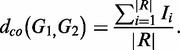
Context–object distance

Suppose G₁ and G₂ are two genomes to be compared; given a structure S, we have their context sets C_S(G₁) and C_S(G₂), respectively. The intersection of the two context sets (denoted by R, use |R| to denote the number of members in R) contains all of the common contexts (Figure 1e). For i from 1 to |R|, let I_i = 0 if object_G1,S(c_i) = object_G2,S(c_i), otherwise let I_i = 1, where c_i is the i^th member of R. The context–object distance (or co-distance) between G₁ and G₂ is given by

(1)

In other words, co-distance is the proportion of shared contexts, the two objects of each of which are different in their respective genomes (Figure 1f).

The algorithm co-phylog and its complexity

The algorithm co-phylog takes as input N genomes G₁, G₂,., G_N, which can be either assembled or not, and the outputs are pairwise co-distances (Figure 1b–f). The algorithm is composed of the following two phases:

1. Convert the input genomes to their respective sets of context–object pairs (Figure 1b–d): given a structure S, for each input genome G in fasta format (assembled genome), we index each O-gram in G by its respective C-gram. If different O-grams with the same C-gram occur while indexing the genome, this C-gram is flagged. After all of the O-grams are indexed, the unmarked C-grams and their respective O-grams, i.e. the context–object pairs, are output. This process is formally expressed by the sub-algorithm fasta2co (see Supplementary Data). For each genome G′ in fastq format (unassembled raw data), we need to first filter low-quality L(S)-tuples. Let W be an L(S)-tuple on a read of G′. If the lowest value of all of the L(S) base qualities of W, denoted by min(W), is smaller than a specific threshold, F, then the W is discarded. For the L(S)-tuples that pass through filtering, the indexing is performed as in fasta2co. This process is formally expressed by the sub-algorithm fastq2co (see Supplementary Data).

2. Compute pairwise co-distances on the sets of context–object pairs using Equation (1) (Figure 1e–f). This process is formally expressed by the sub-algorithm co2distance (see Supplementary Data).

3. Suppose the mean genome size for the N organisms is M_mean and that the mean sequencing depth is d_mean (the depth of the assembled genome is 1), then, at most, phase 1 requires O(M_mean × d_mean × N) time, and phase 2 requires O(M_mean × ) time (see Doc. S1 for the detailed analyses).

4. Once all pairwise co-distances are computed, we use the neighbor-joining (NJ) method (20) to construct phylogenetic trees.

The assessment methods, datasets and benchmarks

The proposed co-phylog algorithm was first assessed using only assembled genomes to explore the proper parameters and the acceptable working range of the algorithm. The algorithm was then assessed on the unassembled whole-genome sequencing data, using the phylogenies based on the corresponding assembled genomes as benchmarks. The full assessment experiments, the corresponding datasets (all of the accession numbers for the datasets used are provided in Supplementary Table S1) and the benchmarks used are introduced below.

Robustness testing by varying context/object lengths on Brucella 13 genomes

We first assessed if the co-phylog method is robust to different context and object lengths. For convenience, we used the simple structures C_a,aO_n with context and object lengths that could be adjusted by choosing different values for a and n, and we only choose a 8 for test, which allowed the majority [>99%, according to Supplementary Equation (S2) in Supplementary Data] of the C-grams to be the contexts. The co-phylog trees were constructed using seven different structures, S = C_8,8O₁, C_9,9O₁, C_10,10O₁, C_12,12O₁, C_15,15O₁, C_15,15O₂ and C_15,15O_4, and took as input the Brucella 13 genomes dataset (including 12 complete genomes from the genus Brucella and an out-group genome from Ochrobactrum anthropi). The resulting trees were then compared with the benchmark tree constructed using the same dataset.

The benchmark tree comes from the work of Foster et al., in which they first created all pairwise whole-genome alignments using MUMmer and then grouped the SNPs by shared locations to compare across all taxa. Foster et al. (21) next analyzed the SNPs multiple alignment using the best substitution model as selected by ModelTest, and finally constructed a phylogenetic tree using the NJ method and verified the tree using different methods.

Tests on the Escherichia/Shigella 26 genomes

We next assessed the algorithm using 26 completed genomes from the genus Escherichia/Shigella. The accuracy of co-phylog was evaluated based on the symmetric differences between the co-phylog (where S = C_9,9O₁) tree and the benchmark tree. Two other phylogenomic tools, CVtree (http://tlife.fudan.edu.cn/cvtree/) and Kr (22) (http://guanine.evolbio.mpg.de/kr2/) were also used to build trees, and the trees’ accuracies were evaluated in the same way. We then made comparisons of the trees’ accuracies among the different phylogenomic methods.

The symmetric differences were evaluated using the ‘treedist’ program that is contained in the PHYLIP package (http://evolution.gs.washington.edu/phylip.html). The benchmark tree that was constructed using the same dataset from the work of Zhou et al. (23), in which they concatenated the alignments of the 2034 core genes of the Escherichia/Shigella 26 genomes and used the maximum likelihood method to infer the phylogenetic relationships.

The accuracy of the co-phylog method was also evaluated via a correlation analysis between the co-distance and the standard p-distance from whole-genomes alignment of the Escherichia/Shigella 26 genomes. Parallel correlation analysis tasks are also implemented using the CVtree-distance and the Kr-distance (as generated by the corresponding tools).

The benchmark p-distances were generated by an in-house Perl script, using the web file 40 way Escherichia/Shigella genomes alignment (http://www.biotorrents.net/details.php?id=87), which includes all the Escherichia/Shigella 26 genomes. This alignment was previously produced by the MSA tool progressiveMauve (24) (http://gel.ahabs.wisc.edu/mauve/).

Tests on Enterobacteriaceae 63 genomes and Gammaproteobacteria 70 genomes

We next examined if the co-phylog method was feasible when applied to high-level taxonomies. In the first stage of the experiment, we tested co-phylog (S = C_9,9O₁) at the family level using 63 genomes randomly picked from Enterobacteriaceae. The reconstructed phylogenetic relationship based on 16S rDNA sequences alignment is used as the benchmark. We then tested co-phylog (S = C_9,9O₁) on the class level using 70 genomes randomly picked from Gammaproteobacteria (we skipped the order level because Enterobacteriaceae is the only family under the order it belongs to). This co-phylog tree was compared with the known taxonomy.

The 16S rDNA tree was generated as follows. For each organism, we first retrieved its 16S rDNA sequence using the ‘Browsers’ on the Ribosomal Database Project (http://rdp.cme.msu.edu/index.jsp) website, and then created MSA of these 16S rDNAs and built a tree using the ‘Tree Builder’ tools (http://rdp.cme.msu.edu/treebuilderpub/index.jsp) (25).

Explore the acceptable working range of co-phylog using in silico evolution

As a complementary experiment to the performance testing on high-level taxonomies, this experiment was designed to provide insights into that how far distant the two compared genomes are would significantly affect the accuracy of the computed co-distance. The artificial life framework, ALF (26), which can simulate the entire range of evolutionary forces (e.g. substitution, indels, gene loss/duplication, GC-content amelioration and lateral gene transfer), was adopted to evolve an ancestor genome into two descendant genomes with a specified evolutionary divergence. The co-distances and the common context counts between the two evolved genomes were then computed. The in silico evolution was repetitively implemented with a gradually increased evolutionary divergence. After the in silico evolution experiments were completed, the relationships between the specified evolutionary divergences and the corresponding co-distances and common context counts were analyzed.

The parameters for ALF simulation were as follows. The ancestor genome, Escherichia coli 536 (NC_008253.ffn), was evolved into two genomes over 150 runs with an initial substitution rate of 0.01 substitutions per site, and each run increased the number of substitutions per site by 0.01 (the rates of other evolutionary events was increased proportionally with the default coefficient defined in the ALF parameters file). The substitution models used were ‘CPAM’ and ‘TN93’ indels: Zipfian; the variation among sites model: rates; the gene number in group later gene transfer (gLGT): 10; and the other parameters follow the default setting.

We were then ready to test co-phylog on NGS data.

Tests on simulated NGS datasets

We first evaluated that how large of a proportion of the genome had to be sequenced to create a faithful tree using co-phylog by in silico sequencing on the ‘sequencing sample genomes’. Supplementary Equation (S1) (see Supplementary Data) suggests that the proportion of the genome sequenced by perfect in silico sequencing could be adjusted through specifying either the mean reads length or the number of reads (or sequencing depth). For convenience, we generated five perfect NGS datasets that only varied in sequencing depth (depth = 2, 6, 16, 30 and 50) using an in-house Perl script and the Brucella 13 genomes as the ‘sequencing sample genomes’. This means that each of the five test NGS datasets consists of 13 unassembled counterparts (G′₁, G′₂,., G′₁₃) at the same depth for the Brucella 13 genomes (G₁, G₂,., G₁₃). All of the reads simulated in the perfect NGS datasets were 75 bp, error-free and uniformly distributed, which allowed us exclude any variation introduced by the sequencing experiment itself. The corresponding co-phylog (with S = C_15,15O₁) tree was constructed using each of the five perfect NGS datasets as input, and the benchmark tree was constructed using the ‘sequencing sample genomes’ as input. The minimal proportion P of the genome that was required by co-phylog was estimated by finding the depth at which the tree generated begins to be identical to the benchmark tree.

When the co-phylog method was applied to a real NGS dataset, L(S)-tuple with a minimum base quality under the threshold F were filtered (see the algorithm section). A dilemma in choosing the F value was that too small of an F might allow too many L(S)-tuple with ‘wrong’ objects past the filtering and therefore enlarge the deviation of the co-distance computed, while too large of an F might filter too much genomic information. We therefore explored the proper value range of F using simulated NGS data with sequencing qualities, which were generated using the tool ‘Maq simulation’ in the MAQ package (http://maq.sourceforge.net/). MAQ NGS data (distinguished from the perfect NGS data, using genome B. abortus 2308) of different depths were generated and different F values were tested on these MAQ NGS data; the proper range of F values were determined according to the co-distance d_co(G′, G) between the MAQ NGS data G′ and the complete genome G and the proportion q of genomic information taken by co-phylog.

Tests on real NGS datasets

Next, we applied co-phylog to the real NGS datasets. By retrieving the NCBI Short Reads Archive database, we collected 29 Escherichia coli organisms for which the NGS raw data and assembled genomes were both available (see Supplementary Table S1). A co-phylog tree constructed using the real NGS dataset for the 29 E. coli organisms was compared with the tree constructed using the respective assembled genomes. We also attempted the co-phylog tool on large diploid genomes to see if co-phylog is computationally affordable to the large size analyses and the additional complication of diploidy. Five mammalian organisms (including four primates, Otolemur garnetii, Saimiri boliviensis, Gorilla gorllia and Homo sapiens, and a out-group Bos grunniens mutus), all of which have abandon NGS data (average sequencing depth 80), were used for phylogenomic analysis by co-phylog. Then the space and time consumption were analyzed.

RESULTS

Performance of co-phylog with varied context/object lengths

The comparison shows that the co-phylog tree and the benchmark tree are nearly identical (Figure 2), illustrating the accuracy of co-phylog method on closely related organisms. It also shows, using S = C_a,aO_n with varied a and n, the co-phylog trees constructed have nearly identical shape, suggesting that co-phylog is robust at different context/object lengths when applied on closely related organisms. However, larger n produces trees with longer branch lengths, and this is because co-phylog method creates a ‘micro-alignment’ between two genomes compared (see ‘Discussion’ section) and estimates the average nucleotide substitution rate that measured by substitutions per n sites, therefore larger n would result in higher substitution rate calculated.

Figure 2.

Comparisons of the alignment-based tree and the co-phylog trees constructed with different structures, on the Brucella 13 genomes. All the trees share the same organisms list. The Ochrobactrum anthropi genome is adopted as the out-group taxon.

Performance on Escherichia/Shigella 26 genomes

Co-phylog tree based on the Escherichia /Shigella 26 genomes shows highly similar topology relative to the benchmark tree (symmetry difference = 4). The branch lengths are proportional to the benchmark tree but shorter (Figure 3a and b). This result occurs because the branch lengths in the co-phylog tree represent the average substitution rates of those sites with unchanged flanking sequences (namely, ‘context’) between two compared genomes, these sites are generally more conserved than the whole-genome average. The most significant difference between CVtree and the other methods is that the genus Shigella violates the monophyleticity of the genus Escherichia but not the monophyleticity of the E. coli strains (symmetry difference = 20). Similar results were also achieved with the FFPs method (15). Note that the CVtree and FFPs distances represent the extent of the difference in the ‘word frequencies’ features of two compared genomes, while co-distance and the alignment-based distance estimate average nucleotide (or amino acid) substitution rate, which is more constant across evolutionary history (see ‘Discussion’ section). One possible explanation is that the CVtree and FFPs trees represent the taxonomy based on genomic features, whereas the co-phylog and alignment-based trees represent the phylogenetic relationship. Another alignment-free method, Kr, was developed to efficiently estimate the pairwise distances between genomes and is ‘more accurate than model-free approaches including the average common substring’ (22). However, according to this test, the Kr tree was still much less accurate than the co-phylog tree as measured by both topology and branch length (Figure 3a), demonstrating the accuracy of co-phylog in establishing the phylogeny of closely related organisms. The only inconsistencies between the co-phylog tree and the benchmark tree were observed on the E. coli CFT073/E. coli 536/E. coli ED1a branch. We found that the difference could be avoided by deleting just E. coli CFT073 (data not shown). It appears that the accuracy of co-phylog methods might be slightly affected if genomes undergo extensive reorganization (such as duplication or recombination) as in the case of E. coli CFT073 (27).

Figure 3.

(a) The benchmark tree constructed based on multiple genomes alignment and the trees constructed by the three methods, co-phylog (S = C_9,9O₁), CVtree and Kr, on the Escherichia/Shigella 26 genomes. The number near the node represents the bootstrap value (see Doc. S1 for details). And (b) the symmetric differences of the benchmark tree against the trees constructed by the three methods, co-phylog, CVtree and Kr. (c) Correlation analyses between the p-distance and each of the three distances, co-distance, CVtree-distance and Kr-distance. These four types of distances are generated from the pairwise comparisons of the Escherichia coli/Shigella 26 genomes, using multiple genomes alignment, co-phylog, CVtree and Kr, respectively.

The correlation analysis indicated that the co-distance fit well with the p-distance (Figure 3c) and had a correlation coefficient of 0.9919. As a comparison, the correlation coefficients versus the p-distance for the other two distances, the CVtree-distance and the Kr-distance are 0.3464 and 0.7796, respectively. The significant linear relationship between the co-distance and the p-distance are also seen in other closely related organisms based on our test data using primate mitochondria DNA alignments (data not shown). This linear relationship explains why the co-phylog tree agrees so well with the alignment-based tree and illustrates that the co-phylog delivers accurate phylogenies of closely related organisms.

Performance on Enterobacteriaceae and Gammaproteobacteria

The comparisons on the phylogenies of the Enterobacteriaceae 63 genomes show that the 16S rDNA tree and the co-phylog tree agreed well in general. However, the genera Enterobacter and Citrobacter are polyphyletic groups, and the genus Yersinia is a paraphyletic group in the 16S rDNA tree, while all these genera formed a single clade in the co-phylog tree, illustrating that co-phylog has a much higher resolution than the 16S rDNA tree at the family level (Figure 4). However, when co-phylog is applied to Gammaproteobacteria 70 genomes, the accuracy of the constructed tree significantly diminishes. Co-phylog tree showed that Enterobacteriales, Xanthomonadales, Pasteurellales and Thiotrichales still formed a clade, whereas the other orders formed paraphyletic or polyphyletic groups (Supplementary Figure S1). The performance on taxonomy levels higher than class were also tested but were found to be even worse than at the class level (data not show). This exercise demonstrates the limits of co-phylog in phylogeny construction.

Figure 4.

Comparison between the 16S rDNA tree and the co-phylog tree, constructed on the Enterobacteriaceae 63 genomes. The number near the node represents the bootstrap value (see Supplementary Data for details).

The optimal working range of co-phylog as determined by in silico evolution

The in silico evolution experiment showed that the co-distance varied significantly starting at the 90th run, which corresponds to a divergence of 0.90 substitutions per site between the two evolved genomes (Figure 5). The major genomic variation introduced in the 90th evolution was a gLGT event that copied 10 genes from one genome to another; the same gLGT event also occurred at the 80th, 74th, 65th and several other previous runs. However, those occurrences did not significantly affect the computed co-distance. The reason is obvious; the sequences ‘copied’ to the genome by the recent gLGT are nearly identical with the original ones on another genome, which causes the co-distance between the two genomes to be underestimated. When two genomes are closely related, there are many common contexts between them; the new common contexts that occurred due to the 10 genes gLGT only affected the co-distance weakly, but two distant genomes have few common contexts (e.g. 5000), and the new common contexts that occurred owing to a 10 genes gLGT (∼10 000 common contexts) would make up the majority of the common contexts, thus significantly biasing the computed co-distance. This experiment indicates that when the common context count 150 000 (corresponding to a co-distance 0.12 or a real divergence of 0.8 substitution per site if S = C_9,9O₁), the two genomes being compared are close enough to guarantee the stability of the computed co-distance. If using S = C_12,12O₁, then ‘close enough’ genomes should satisfy the criteria of the divergence being 0.58 substitution per site and have a co-distance 0.09, indicating that using long contexts loses more distant homologies. Therefore, when the criteria given in Supplementary Equation (S2) (see Supplementary Data) are satisfied, it is better to choose shorter contexts when applying co-phylog to more distant genomes. This estimation may be different when taking into account more frequent, recent gLGTs. Fortunately, relevant research has suggested that recent gLGTs in two distant genomes are rare (about 7 genes) (28), making the conclusions from our 10-gene gLGT simulation more reliable.

Figure 5.

The changing of the co-distances and the log number of the common context counts computed between two genome evolved in silico, with gradually increased evolutionary divergence (substitutions per codon), using two structures S = C_9,9O₁ and C_12,12O₁.

Performance on simulated NGS datasets

Through comparing the co-phylog trees constructed using the perfect NGS datasets with the benchmark tree (Supplementary Figure S2a). We found that when the perfect NGS datasets are ‘deeper’ than 6, the co-phylog tree generated is identical to the benchmark tree. Using B.abortus 2308 (one of the Brucella 13 genomes; the other 12 genomes are of similar lengths) as a representation, the L(S)-tuples count of the complete B.abortus 2308 genome G is |H_k,G| = 6 485 644, and the 6 perfect NGS data G′ of the B.abortus 2308 genome generated |H_k,G′| = 6 366 349; therefore, the proportion q of L(S)-tuples in |H_k,G| that were included in |H_k,G′| is 0.98 (see the ‘The k-tuples set’ section for the definitions of |H_k,G| and |H_k,G′|), which indicates that the minimal proportion, P, of the genome required by co-phylog is ∼0.98. This value is close to a proportion of 0.97 estimated by Supplementary Equation (S1), illustrating the accuracy of Supplementary Equation (S1) (see Supplementary Data).

The experiment on the MAQ NGS data G′ of the B. abortus 2308 genome G shows that the smaller the qualities filter threshold F is or the ‘deeper’ the MAQ NGS data are, the larger the computed co-distance d_co(G′, G) is (Table 1), as anticipated. Suppose that G′₁ and G′₂ are the NGS data generated from the ‘sequencing sample genomes’ G₁ and G₂, respectively. According to the triangle inequality, we have d_co(G′₁, G′₂) d_co(G′₁, G₂) d_co(G₂, G′₂) d_co(G₁, G₂) d_co(G₁, G′₁) d_co(G₂, G′₂); therefore,

(2)

Table 1.

The co-distances d_co(G′, G) and the proportion q% (the bracketed value) of L(S)-tuples taken by co-phylog computed for each depth-F combination

F	The depths of the MAQ NGS data
	2	6	16	30	50
0	6.5e-05 (70.0)	1.1e-04 (97.1)	2.8 e-04 (100)	5.1 e-04 (100)	8.7 e-04 (100)
5	5.3e-06 (57.8)	1.1e-05 (92.4)	1.6 e-05 (99.9)	3.0 e-05 (100)	5.0 e-05 (100)
10	3.3e-06 (46.2)	5.5e-06 (84.2)	8.4 e-06 (99.3)	1.4e-05 (100)	1.8 e-05 (100)
15	3.9e-06 (31.4)	3.2e-06 (67.5)	3.9 e-06 (95.0)	4.3 e-06 (99.6)	9.2 e-06 (100)
20	2.6e-06 (11.2)	2.0e-06 (31.2)	2.0 e-06 (63.4)	2.5 e-06 (84.7)	1.3 e-06 (95.5)
25	0 (2.3)	4.6e-06 (6.7)	1.8 e-06 (17.3)	0 (29.6)	7.0 e-07 (44.3)
30	0 (0.02)	0 (0.04)	0 (0.11)	0 (0.21)	0 (0.33)
35	NA (0)	NA (0)	NA (0)	NA (0)	NA (0)

NA represents that the d_co(G′, G) cannot be computed because there is no L(S)-tuples taken.

Equation (2) illustrates that the co-distance, d_co(G′, G), determines the extent to which the co-distance computed using NGS data deviates from the real co-distance of the two compared genomes and therefore determines the limit of the resolution of the constructed co-phylog tree. For the phylogenetic analysis at the genus or species level, d_co(G′, G) 1e-5 ensure sufficiently high resolution and is therefore adopted as a criterion for choosing F. Combining this d_co(G′, G) criterion and the minimal required genome proportion previously inferred and considering that the NGS data generated from most bacterial sequencing projects would be higher than 16, an F from 10 to 15 should be sufficient for practical usage.

Once the proper F value range was determined, we then tested the performance of co-phylog with arbitrarily selected parameters within the allowed value range (S = C_15,15O₁, F = 10) using the MAQ NGS data that are ‘deeper’ than 16 as input. We considered that, in practice, co-phylog will likely deal with NGS data from various independent sequencing projects; we therefore generated a ‘mixed depth’ testing dataset in which the NGS data of the Brucella 13 genomes were of different depths for the different organisms (the depth were specified arbitrarily provided that they were all ‘deeper’ than 16). As we anticipated, the co-phylog tree based on this ‘mixed depth’ testing dataset was identical with the benchmark tree (Supplementary Figure S2b).

Unassembled reads generally contain a significant number of sequencing errors, polymerase chain reaction (PCR) amplification redundancies and even contaminations. These effects were also evaluated: the extent of their impact was measured by the deviations between the benchmark co-distance (computed using assembled genomes, S = C_9,9O₁) and the corresponding co-distance (with parameters S = C_9,9O₁, F = 10) computed using NGS data simulated with different coverages and effects (Table 2). This analysis showed that the impacts of sequencing errors and PCR amplification redundancies on the proposed algorithm are negligible, but the impact of contaminations cannot be neglected.

Table 2.

The extents of co-distance biases due to sequencing error, PCR and contamination

Coverage	Error ratea (%)				PCRb	Contamination levelsc (%)
	0.01	0.05	0.1	1		1	2	3
20	0	0	0	2.6e-05	1.2e-05
50	0	4e-06	8e-06	0.000159	0
100	0	0	2e-05	0.000671	0	0.0015	0.0036	0.0053

^aThe benchmark co-distance (0.018) was computed between genomes E. coli 536 and E. coli K12, and their NGS data were simulated with different coverages and error rates by the tool ‘Art’ (29). The error rates of popular NGS platforms ranged from 0.01 to 1%, according to (30).

^bNGS data simulated with biased PCR amplification were generated using the tool ‘pirs’, which incorporated the coverage GC-content profile trained based on real NGS data (31).

^cThe simulated scenario was that both NGS data sets (generated from genomes Shigella boydii and Shigella flexneri, with benchmark co-distance 0.009) were contaminated by the sequences from E. coli K12. Then the co-distance was computed between the two contaminated NGS samples (add up to 100× coverage for each sample). The contamination levels represent the proportions of the E. coli K12 sequences.

Performance on real NGS datasets

The co-phylog (S = C_9,9O₁, qualities control threshold F = 10) tree constructed using the NGS raw dataset of the 29 E. coli organisms is almost identical to the tree built using the corresponding assembled genomes (Figure 6). Given the accuracy of the co-phylog method based on assembled genomes has been proved previously, this test illustrates that co-phylog could be used in the phylogenetic analysis of unassembled NGS data. And as these NGS raw data came from all three popular sequencing platforms (454, Illumina and SOLID) (Supplementary Table S1), co-phylog is robust to the choice of sequencing platforms. The co-phylog tree (using S = C_12,12O₁, according to Supplementary Equation (S2) and F = 10) constructed on the NGS dataset from the five large diploid organisms matched well with the known taxonomy (Supplementary Figure S3), illustrating that the tool co-phylog can handle large size analyses and the complication of diploidy.

Figure 6.

Comparison between the co-phylog tree constructed using assembled genomes of the E. coli 29 organisms and the co-phylog tree constructed using their corresponding NGS raw data. The Escherichia fergusonii genome is adopted as the out-group taxon.

The time and memory consumption of co-phylog program (coded in C) were tested on a platform equipped with Intel Xeon X5650 2.67 GHz cpu (only one cpu was used for this test) and SUSE Linux Enterprise Server 10 SP2 (×86_64). For real NGS dataset from the E. coli 29, which have an average sequencing depth of 95, co-phylog took 160M memory and 19 min completing the whole computing, including 14 min converting all NGS data into corresponding context–object sets and 5 min computing all pairwise co-distances. For the five mammalian organisms, co-phylog took 60G memory and 20 h completing the whole computing, including 17 h converting all NGS data into corresponding context–object sets and 3 h computing all pairwise co-distances.

DISCUSSION

The context–object model is a ‘micro-alignment’ process

As we have previously introduced, the traditional sequences alignment method is a ‘seed match then extend’ process. Recall that for computing the co-distance between two genomes G₁ and G₂, each member c_i in the intersection R of the two context sets, C_S(G₁) and C_S(G₂), is a context match that corresponds to the seed match in a spaced seed alignment. Unlike traditional alignment, the context–object model does not extend inter-seeds but instead extends intra-seeds (namely, the O-parts of the structure). Because the O-parts are short (typically 1 or a few base pairs), it is reasonable to ignore indels during extension. Extension is therefore directly comparing O-grams, and the context–object model is an alignment process with a span of only ∼20∼30 bp, a so-called ‘micro-alignment’.

There are two main features that make micro-alignment much more efficient than traditional alignment. First, a context match is created only once between the two compared genomes, while a normal ‘seed match’, which is shorter, is created many times in different regions, which slows down the calculation (19). Second, once a context match is created, as we have elaborated, extensions can be implemented by comparing two O-grams directly. As an O-gram can be stored in a ‘word’, an extension requires only one operation. In traditional alignment method, the seed match is extended through a dynamic programming process that requires polynomial operations.

Micro-alignments do share a problem with the traditional alignment, namely that the homologies searching by using longer seed (or structure S) would lose distant homologies (19). This problem is more severe in micro-alignments because the C part of structure S must be long enough to ensure most C-grams from a genome can be mapped back to a unique region of the genome (therefore, to be the contexts), with increased genetic differences of the involved genomes, the counts of common context and phylogenetic information decreased more dramatically, which hindered the application of the proposed approach to far distant organisms.

Comparison against alignment-free methods

Intuitively, the co-phylog method is somewhat similar to several alignment-free methods, especially those word frequencies methods. For example: Edgar et al. first compute the normalized common k-tuples count F(X,Y), from the common k-tuples C_i^XY between two sequences X and Y, using the following equation:

(3)

where = |{A, C, G, T}|^k, for DNA sequences comparisons, and n and m are the lengths of X and Y, respectively. This was then transformed into a distance, d_F(X, Y) = −log(0.1 + F) (32). The similar calculation formulas of co-distance (Equation (1)) and the d_F(X, Y) implies they have similar computing efficiency. However, their biological meanings are essentially different. As we have previously elaborated, the context–object model is a micro-alignment process, which allows co-phylog to only call the nucleotide substitution events out of the entire range of genome variation. Therefore the co-distance computed, according to Equation (1), estimated the whole-genome average nucleotide (or amino acid) substitution rate of those sites with unchanged flanking sequences (namely, ‘context’) between the two genomes compared. The calling of substitution events is critical for accurately constructing phylogenetic trees because the nucleotide (or amino acid) substitution rate is relatively constant across evolutionary history according to the molecular clock hypothesis. In contrast, the normalized common k-tuples F(X,Y) could be affected by a wide range of genome variation events to different extents. For example, a gene lost event could decrement thousands of common k-tuples, C_i^XY, while a nucleotide substitution event could decrement only a few common k-tuples, the changes in are obviously not proportional with that of C_i^XY, thereby the F(X,Y) or d_F(X, Y) computed do not represent the rate of any evolutionary event. There is no unified evolution model for all of the types of genomic variations; therefore, the alignment-free distance metric, which do not distinguish between different types of genome variations cannot be accurate.

In conclusion, the advantages and limitations of co-phylog method are obvious. co-phylog has similar computing efficiency with ‘word frequencies’ based on alignment-free methods, and in the mean time, it shares the accuracy with other alignment-based methods. However, co-phylog method does not perform well on far distant organisms.

SUPPLEMENTARY DATA

Supplementary Data are available at NAR Online: Supplementary Methods, Supplementary Table 1 and Supplementary Figures 1–3.

FUNDING

National Basic Research Program [2012CB944600]; Ministry of Science and Technology [2011BAI09B00]; Ministry of Health [201002007]; National Science Foundation of China [30890034]; Ministry of Education [311016]; National High-Tech Research and Development Program [2012AA021802] and National Science Foundation of China [31271338]. Funding for open access charge: National Basic Research Program [2012CB944600].

Conflict of interest statement. None declared.

REFERENCES

- 1.Wiens JJ. Missing data, incomplete taxa, and phylogenetic accuracy. Syst. Biol. 2003;52:528–538. doi: 10.1080/10635150390218330. [DOI] [PubMed] [Google Scholar]
- 2.Snel B, Bork P, Huynen MA. Genome phylogeny based on gene content. Nat. Genet. 1999;21:108–110. doi: 10.1038/5052. [DOI] [PubMed] [Google Scholar]
- 3.Blanchette M, Kunisawa T, Sankoff D. Gene order breakpoint evidence in animal mitochondrial phylogeny. J. Mol. Evol. 1999;49:193–203. doi: 10.1007/pl00006542. [DOI] [PubMed] [Google Scholar]
- 4.Ulitsky I, Burstein D, Tuller T, Chor B. The average common substring approach to phylogenomic reconstruction. J. Comput. Biol. 2006;13:336–350. doi: 10.1089/cmb.2006.13.336. [DOI] [PubMed] [Google Scholar]
- 5.Qi J, Wang B, Hao BI. Whole proteome prokaryote phylogeny without sequence alignment: a K-string composition approach. J. Mol. Evol. 2004;58:1–11. doi: 10.1007/s00239-003-2493-7. [DOI] [PubMed] [Google Scholar]
- 6.Hohl M, Ragan MA. Is multiple-sequence alignment required for accurate inference of phylogeny? Syst. Biol. 2007;56:206–221. doi: 10.1080/10635150701294741. [DOI] [PMC free article] [PubMed] [Google Scholar]
- 7.Loytynoja A, Goldman N. Phylogeny-aware gap placement prevents errors in sequence alignment and evolutionary analysis. Science. 2008;320:1632–1635. doi: 10.1126/science.1158395. [DOI] [PubMed] [Google Scholar]
- 8.Wong KM, Suchard MA, Huelsenbeck JP. Alignment uncertainty and genomic analysis. Science. 2008;319:473–476. doi: 10.1126/science.1151532. [DOI] [PubMed] [Google Scholar]
- 9.Elias I. Settling the intractability of multiple alignment. J. Comput. Biol. 2006;13:1323–1339. doi: 10.1089/cmb.2006.13.1323. [DOI] [PubMed] [Google Scholar]
- 10.Wang L, Jiang T. On the complexity of multiple sequence alignment. J. Comput. Biol. 1994;1:337–348. doi: 10.1089/cmb.1994.1.337. [DOI] [PubMed] [Google Scholar]
- 11.Stuart GW, Berry MW. A comprehensive whole genome bacterial phylogeny using correlated peptide motifs defined in a high dimensional vector space. J. Bioinform. Comput. Biol. 2003;1:475–493. doi: 10.1142/s0219720003000265. [DOI] [PubMed] [Google Scholar]
- 12.Li M, Badger JH, Chen X, Kwong S, Kearney P, Zhang H. An information-based sequence distance and its application to whole mitochondrial genome phylogeny. Bioinformatics. 2001;17:149–154. doi: 10.1093/bioinformatics/17.2.149. [DOI] [PubMed] [Google Scholar]
- 13.Chen X, Kwong S, Li M. A compression algorithm for DNA sequences and its applications in genome comparison. Genome Inform. Ser. Workshop Genome Inform. 1999;10:51–61. [PubMed] [Google Scholar]
- 14.Otu HH, Sayood K. A new sequence distance measure for phylogenetic tree construction. Bioinformatics. 2003;19:2122–2130. doi: 10.1093/bioinformatics/btg295. [DOI] [PubMed] [Google Scholar]
- 15.Jun SR, Sims GE, Wu GA, Kim SH. Whole-proteome phylogeny of prokaryotes by feature frequency profiles: an alignment-free method with optimal feature resolution. Proc. Natl. Acad. Sci. USA. 2010;107:133–138. doi: 10.1073/pnas.0913033107. [DOI] [PMC free article] [PubMed] [Google Scholar]
- 16.Cannon CH, Kua CS, Zhang D, Harting JR. Assembly free comparative genomics of short-read sequence data discovers the needles in the haystack. Mol. Ecol. 2010;19(Suppl. 1):147–161. doi: 10.1111/j.1365-294X.2009.04484.x. [DOI] [PubMed] [Google Scholar]
- 17.Ratan A, Zhang Y, Hayes VM, Schuster SC, Miller W. Calling SNPs without a reference sequence. BMC Bioinformatics. 2010;11:130. doi: 10.1186/1471-2105-11-130. [DOI] [PMC free article] [PubMed] [Google Scholar]
- 18.Peterlongo P, Schnel N, Nadia P, Sagot M-F, Vincent L. Identifying SNPs without a reference genome by comparing raw reads. In: Chavez E, Lonardi S, editors. String Processing and Information Retrieval—17th International Symposium. 2010. Vol. 6393. Los Cabos, Mexico, pp. 147–158. [Google Scholar]
- 19.Ma B, Tromp J, Li M. PatternHunter: faster and more sensitive homology search. Bioinformatics. 2002;18:440–445. doi: 10.1093/bioinformatics/18.3.440. [DOI] [PubMed] [Google Scholar]
- 20.Saitou N, Nei M. The neighbor-joining method: a new method for reconstructing phylogenetic trees. Mol. Biol. Evol. 1987;4:406–425. doi: 10.1093/oxfordjournals.molbev.a040454. [DOI] [PubMed] [Google Scholar]
- 21.Foster JT, Beckstrom-Sternberg SM, Pearson T, Beckstrom-Sternberg JS, Chain PS, Roberto FF, Hnath J, Brettin T, Keim P. Whole-genome-based phylogeny and divergence of the genus Brucella. J. Bacteriol. 2009;191:2864–2870. doi: 10.1128/JB.01581-08. [DOI] [PMC free article] [PubMed] [Google Scholar]
- 22.Domazet-Loso M, Haubold B. Efficient estimation of pairwise distances between genomes. Bioinformatics. 2009;25:3221–3227. doi: 10.1093/bioinformatics/btp590. [DOI] [PubMed] [Google Scholar]
- 23.Zhou Z, Li X, Liu B, Beutin L, Xu J, Ren Y, Feng L, Lan R, Reeves PR, Wang L. Derivation of Escherichia coli O157:H7 from its O55:H7 precursor. PLoS One. 2010;5:e8700. doi: 10.1371/journal.pone.0008700. [DOI] [PMC free article] [PubMed] [Google Scholar]
- 24.Darling AE, Mau B, Perna NT. ProgressiveMauve: multiple genome alignment with gene gain, loss and rearrangement. PLoS One. 2010;5:e11147. doi: 10.1371/journal.pone.0011147. [DOI] [PMC free article] [PubMed] [Google Scholar]
- 25.Cole JR, Wang Q, Cardenas E, Fish J, Chai B, Farris RJ, Kulam-Syed-Mohideen AS, McGarrell DM, Marsh T, Garrity GM, et al. The Ribosomal Database Project: improved alignments and new tools for rRNA analysis. Nucleic Acids Res. 2009;37:D141–D145. doi: 10.1093/nar/gkn879. [DOI] [PMC free article] [PubMed] [Google Scholar]
- 26.Dalquen DA, Anisimova M, Gonnet GH, Dessimoz C. ALF–a simulation framework for genome evolution. Mol. Biol. Evol. 2012;29:1115–1123. doi: 10.1093/molbev/msr268. [DOI] [PMC free article] [PubMed] [Google Scholar]
- 27.Touchon M, Hoede C, Tenaillon O, Barbe V, Baeriswyl S, Bidet P, Bingen E, Bonacorsi S, Bouchier C, Bouvet O, et al. Organised genome dynamics in the Escherichia coli species results in highly diverse adaptive paths. PLoS Genet. 2009;5:e1000344. doi: 10.1371/journal.pgen.1000344. [DOI] [PMC free article] [PubMed] [Google Scholar]
- 28.Wagner A, de la Chaux N. Distant horizontal gene transfer is rare for multiple families of prokaryotic insertion sequences. Mol. Genet. Genomics. 2008;280:397–408. doi: 10.1007/s00438-008-0373-y. [DOI] [PubMed] [Google Scholar]
- 29.Huang W, Li L, Myers JR, Marth GT. ART: a next-generation sequencing read simulator. Bioinformatics. 2012;28:593–594. doi: 10.1093/bioinformatics/btr708. [DOI] [PMC free article] [PubMed] [Google Scholar]
- 30.Glenn TC. Field guide to next-generation DNA sequencers. Mol. Ecol. Resour. 2011;11:759–769. doi: 10.1111/j.1755-0998.2011.03024.x. [DOI] [PubMed] [Google Scholar]
- 31.Hu X, Yuan J, Shi Y, Lu J, Liu B, Li Z, Chen Y, Mu D, Zhang H, Li N, et al. pIRS: profile-based Illumina pair-end reads simulator. Bioinformatics. 2012;28:1533–1535. doi: 10.1093/bioinformatics/bts187. [DOI] [PubMed] [Google Scholar]
- 32.Edgar RC. Local homology recognition and distance measures in linear time using compressed amino acid alphabets. Nucleic Acids Res. 2004;32:380–385. doi: 10.1093/nar/gkh180. [DOI] [PMC free article] [PubMed] [Google Scholar]
Associated Data
This section collects any data citations, data availability statements, or supplementary materials included in this article.