Ensuring the statistical soundness of competitive gene set approaches: gene filtering and genome-scale coverage are essential

Abstract

In this article, we focus on the analysis of competitive gene set methods for detecting the statistical significance of pathways from gene expression data. Our main result is to demonstrate that some of the most frequently used gene set methods, GSEA, GSEArot and GAGE, are severely influenced by the filtering of the data in a way that such an analysis is no longer reconcilable with the principles of statistical inference, rendering the obtained results in the worst case inexpressive. A possible consequence of this is that these methods can increase their power by the addition of unrelated data and noise. Our results are obtained within a bootstrapping framework that allows a rigorous assessment of the robustness of results and enables power estimates. Our results indicate that when using competitive gene set methods, it is imperative to apply a stringent gene filtering criterion. However, even when genes are filtered appropriately, for gene expression data from chips that do not provide a genome-scale coverage of the expression values of all mRNAs, this is not enough for GSEA, GSEArot and GAGE to ensure the statistical soundness of the applied procedure. For this reason, for biomedical and clinical studies, we strongly advice not to use GSEA, GSEArot and GAGE for such data sets.

INTRODUCTION

The analysis of gene sets for detecting an enrichment of differentially expressed genes has received much attention in the past few years. One reason for this interest can be attributed to the general shift of focus within the biological and biomedical sciences toward systems properties (1) of molecular and cellular processes (2–7). It is now generally acknowledged that statistical methods for analyzing gene expression data that aim to detect biological significance need to capture information that is consequential for the emergence of a biological function. For this reason, methods for detecting the differential expression of (individual) genes have less explanatory power than methods based on gene sets (8), especially if these gene sets correspond to biological pathways (9). For the following discussion, we assume that the definition of the gene sets is based on biologically sensible information about pathways as obtained, e.g. from the gene ontology (GO) database (10), MSigDB (11), KEGG (12) or expert knowledge.

Many methods have been suggested for detecting the differential expression of gene sets or pathways (8,13–19). These methods can be systematically classified based on different characteristics (e.g. univariate or multivariate, parametric or non-parametric) (20,21), but the most important difference between different approaches is whether they are ‘self-contained’ or ‘competitive’ (21). Self-contained tests use only the data from a target gene set under investigation, whereas competitive tests use, in addition, data ‘outside’ the target gene set, which can be seen as background data. This appears curious, and one might ask whether the term ‘background data’ is well defined. One purpose of this article is to demonstrate that a precise definition of the ‘background data’ is necessary to avoid a statistical misconception for the usage of competitive tests.

The present article focuses on competitive gene set methods, investigating their inferential characteristics. More precisely, we study the five competitive gene set methods GSEA (11), GSEArot (22), ‘random set’ (23), GAGE (24) and GSA (25), and investigate their ‘power’ and ‘false-positive rate’ (FPR) with respect to biological and simulated data sets. The reason for selecting these five methods is that GSEA is currently arguably thus far the most popular gene set method, which is frequently applied to biological and biomedical data set. The methods GSEArot and GSA are closely respectively distantly related to GSEA, claiming to provide an improvement of the statistical methodology aiming for an enhanced detection capability of biological significance. In contrast to GSEA, GSEArot and GSA, which are three non-parametric methods, ‘random set’ and GAGE are parametric methods. Including the methods ‘random set’ and GAGE in our analysis allows studying the influence of these different types of statistical inference methodologies on the outcome of competitive tests. For example, for microarray data with large sample sizes, non-parametric methods based on a resampling of the data are frequently recommended, resulting in a better performance than comparable parametric methods (26,27). However, it is currently unknown whether competitive non-parametric tests have more power than competitive parametric tests.

The major purpose of this article is to investigate the performance of these five methods, depending on (i) the correlation structure in the data, (ii) the effect of up- and down-regulation of genes, (iii) the influence of the background data (gene filtering) and (iv) the influence of the sample size. These dependencies are of particular biological relevance because these conditions are known to vary widely among data sets of different origin, e.g. owing to physiological conditions, patho- or tumorigenesis, medication of drugs or even the preprocessing of the data. Thus far, several studies compared competitive gene set methods with each other (20,21). However, in our analysis, we choose more expressive conditions to reveal the underlying methods’ characteristics relentlessly. A schematic overview of our analysis is shown in Figure 1, and the parameters we will study are highlighted in red. A detailed discussion of the various aspects of our analysis and the categorization of data is given at the beginning of the ‘Results’ section.

Figure 1.

Schematic overview and visualization of the analysis conducted in this article. The analysis focuses of our study are highlighted in red (A–D).

The article is organized as follows. In the ‘Materials and Methods’ section, we describe the data we are using for our analysis, and introduce the error measure that are relevant for their quantitative assessment. The ‘Results’ section is subdivided into four major parts. In the first two subsections, we use data from prostate cancer to study the influence of the correlation structure in the data, the effect of the up- and down-regulation of genes and the overall influence of the sample size (A, B and D in Figure 1). The following two subsections focus on the influence of background data and the importance of data filtering (C in Figure 1). For this analysis, we are using microarray data from acute lymphoblastic leukemia (ALL), prostate cancer and breast cancer as well as simulated data sets. The article finishes with the ‘Discussion’ section summarizing our results and providing recommendations for the practical usage of the studied methods.

MATERIALS AND METHODS

In this section, we describe the biological and simulated data we use for our analysis.

Surrogate data: prostate cancer

To investigate the dependency of gene set methods’ performance on (i) the correlation structure in the data, (ii) the effect of up- and down-regulation of genes and (iii) the influence of the background data, we generate six different data sets. In the next section, we describe how these data sets are defined, and in section ‘Generation of surrogate data’, we define a bootstrap procedure we apply to these data to generate surrogate data.

Preparation of data with a biological pathway partitioning

We use a gene expression data set of prostate cancer from (28) generated from an Affymetrix platform. For the preprocessing and normalization of the data, we followed (28). We use this data set as a reference data set and call it D_F. D_F consists of two expression matrices X^t (treatment group) and X^c (control group) of dimension (p × n_t) and (p × n_c), respectively, with p = 8727 genes and n_t = 52 samples for the treatment and n_c = 50 samples for the control group. Here, the number of genes p refers to the genes that pass the filtering of the preprocessing of the data [interquartile range (IQR) = 0.4]; hence, this number is different from the number of genes present on the chip. For this reason, we index the data set by an ‘F’ (filtered). We call the total number of genes on the chip q(12 625). For our analysis, we use equal sample sizes n = n_t = n_c = 50 for the control and treatment group by randomly selecting 50 samples from the 52 treatment group. After the normalization, we map the genes to the category ‘biological process’ of level four in the GO database (10) to obtain information about their association with biological pathways. For the prostate cancer data set, we identify 213 different pathways.

From D_F, we generate a data set without a correlation structure between the genes by applying the following procedure:

• To generate expression data with the same distribution of expression values for each gene, but without a correlation structure, we permute each row vector of the two matrices X^t and X^c independently, for each gene. That means we permute the sample labels, independently for each gene and the treatment and control group. We call the resulting data set .

It is important to note that the two data sets are paired . This becomes important when we compare results for D_F with in section ‘Robustness of the methods’. Furthermore, we would like to remark that the data set generated by this procedure is similar to the prostate cancer data because it maintains individual gene scores, e.g. t-scores. However, the important difference is that the genes in this data set are uncorrelated.

To study the effect of the up- and down-regulation of genes, we generate another data set called . This data set is obtained by ordering all genes in the data set D_F in such a way that we have only up-regulated genes.

• For each gene in D_F, we compare the mean expression value of a gene between the treatment and the control group. If we find a down-regulated gene in the treatment group, the gene expression profiles between the treatment and the control group are replaced with each other, for this gene only. This procedure results in a data set, called , that contains only up-regulated genes with respect to the treatment group that means the proportion of up-regulated genes is one.

Finally, to study the influence of the background data, we use the prostate cancer data set consisting of all q genes present on the microarray chip. We call this data set D_A (for ‘all’ genes). We apply to D_A the same procedures as for D_F to obtain uncorrelated () and up-regulated () data. This gives six different data sets (D_F, , D_A, ) that maintain important characteristics of real data, including their membership to the biological pathways, despite the various transformations we apply to the original data sets D_F and D_A.

Generation of surrogate data

For analyzing each of the six data sets—in the following, we use the shortcut D to indicate —we apply a two-step strategy.

First, we use a data set D(n) (of sample size n = 50) and identify which pathways are significant and which are not. We call the resulting list of significant pathways and the list of pathways that are non-significant . That means, for each pathway , we consider its null hypothesis as truly false, i.e. H₀(i,n) = 1. To emphasize the dependency of this result on the sample size, we write the pathway lists and the null hypotheses as a function of n. For the following analysis, we use the results from this analysis as reference lists, as we consider the significant pathways in as ‘true positives’ and the non-significant pathways in as ‘true negatives’. In the second step, we construct b(n_k) = 100 bootstrap data sets for k = 9 different sample sizes, (step size: 5), whereas each data set is drawn from the total of n available samples. To each bootstrap data set, we apply a gene set method. From this, a result is assessed with respect to the reference lists, and , obtained for sample size n, in Step 1.

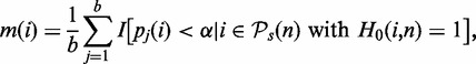
More precisely, we calculate the power of a test for a given sample size n_k by calculating the P-values, p_j(i), for the pathways with H₀(i,n) = 1 ( and ). From this, we estimate the ‘mean proportion of significant results’ from the b bootstrap samples,

(1)

assessed at a significance level of α = 0.05. Here I() is the indicator function, which is ‘1’ if its argument is true and ‘0’ otherwise. Furthermore, m(i) corresponds to the power of the test with respect to pathway i . To obtain the power of the test with respect to arbitrary pathways, we average over all significant pathways,

(2)

This provides an estimate for the probability to reject the null hypothesis when the null hypothesis is false, which corresponds to the power of the test with respect to . We would like to emphasize that this is not the (true) power of a test, which is defined with respect to the true list of significant pathways, ,

(3)

Similarly, we estimate the FPR of a test from the P-values of the pathways with true null hypothesis with respect to the reference list .

We would like to point out that owing to the fact that our reference list may contain false declarations, our results assess the ‘statistical robustness’ of the tests, by providing estimates for, e.g. their power, rather than their true value. Furthermore, because we generate bootstrap data sets for each sample size n_k, we consider these as surrogate data for newly generated data from independent experiments, which are not available.

RESULTS

To simplify the following discussions, we introduce first some notation. Generally, all competitive gene set methods, which are discussed in detail in the supplementary file in the ‘Methods’ section, use genes in a target (t) gene set W (see Figure 1). We term the contributing expression data for this target pathway D_t = D(W), and the data from a background (b) gene set D_b. Depending on the method, see ‘Materials and Methods’ section, D_b is either given by D(W^c) or D(V), whereas V corresponds to the set of all genes used for an analysis, and W^c is the complementary set of genes given by W^c = V − W (set difference). Hence, for every analyzed pathway, a data set D is split into two data sets, D_t and D_b, which are not necessarily mutually exclusive. We want to emphasize that neither D_t nor D_b are fixed, but they change their roles for every target pathway, W, that is analyzed.

Interestingly, there is a second separation of the data possible that is important for our study. This separation refers to a non-overlapping separation of D into experimental (e) data, D^e, and unrelated (u) data, D^u, i.e. . Here, by experimental data, we mean data that convey information about an experiment. In contrast, unrelated data represent essentially noise without information about the underlying experiment. Specifically, for microarray data, genes that are at least on a basal level expressed carry information, and hence, contribute to experimental data. In contrast, not every gene in a genome is expressed. Nevertheless, such genes may lead to non-vanishing expression values, e.g. owing to cross-hybridization. However, such gene expressions are considered as unrelated data. In Figure 1, the data D^e and D^u are visualized as violet ellipses and green rectangles, respectively. On the level of cellular networks, the non-expression of genes is indicated by the absence of connections (interactions) between genes. Hence, such genes do not contribute to the cellular networks for the physiological condition under investigation. In contrast, genes that are expressed interact with each other by forming cellular networks. In Figure 1, gene expression is measured only for the genes that are part of the cellular network that has a green underlay.

Practically, one aims to separate D^e and D^u from each other by applying a filtering procedure to an expression data set. This separation is mutually exclusive because either the expression value of a gene contains information or it does not. Also, this separation is fixed for a given data set D; hence, it is independent of any target pathway.

These two types of data separations, as defined above, can be intertwined with each other. For example, suppose a data set has either not been filtered or the filtering criterion was too loose, resulting in the presence of genes that are not expressed at all (here we do not speak about differential expression, but a lack of a basal expression). In such a case, a data set D consists of both parts D^e and D^u. This implies that every data set D_t of a target pathway can also be separated in such two parts, namely, and , and similarly the background data for this target pathway separates in and .

That means there are non-trivial data separations that can be considered, and in the following, we will see that competitive gene set methods can be only fully understood in terms of these data separations.

Influence of correlation and expression: filtered data

In Figure 2, we show results for the surrogate data of prostate cancer for the three filtered data sets D_F (top row), (middle row) and (bottom row). The colors of the curves correspond to GSEA (red), GAGE (green), GSA (blue), ‘random set’ (gold) and GSEArot (purple). With respect to the notation introduced above, this means that the data for the target pathway as well as for the background contain (approximately) only information from experimental data, i.e. and , for all tested pathways.

Figure 2.

Prostate cancer: results for D_F (top row), (middle row) and (bottom row). Shown are the power (first column), FPR (second column) and the ‘number of significant pathways’ (third column) for different pathway-based methods. GSEA (red), GAGE (green), GSA (blue), ‘random set’ (gold) and GSEArot (purple).

From this figure, one can see that the power of GAGE (green) seems to be least affected by the different transformations of the data, resulting in a similar power for all three data sets. However, the number of significant pathways for and is reduced by ∼50% compared with D_F, which means that the number of detected ‘true positive’ pathways for and is reduced by a factor of 2. The power of ‘random set’ (gold) is similar for D_F and , but reduced for . Also, the number of significant pathways for is reduced by >50%.

The number of significant pathways for GSEA (red) and GSEArot (purple) is the smallest compared with all other methods. It is interesting to note that the power of GSEA for the data set is larger than for the other two data sets (D_F and ), i.e. reducing the correlation in the data leads to an increase in the power and also in the number of significant pathways. The reason for this behavior is that the correlation has an influence on the data. The correlation structure between gene profiles increases the gene set scores and increases false-positive predictions (29). The power of GSA (blue) appears to be stable across the different transformations, but the changing numbers of significant pathways indicate otherwise. We come back to this point in the section ‘Robustness of the methods’.

In general, for large sample sizes, the FPR is well controlled by all methods. For small sample sizes, ‘random set’ (gold) attains the largest FPR of ∼10%. This may come from the parametric nature of this test, and hint to deviations of assumption with respect to the real characteristics of the data.

Robustness of the methods

To investigate the influence of the filtering on the results, we repeated a similar analysis as above, but for the unfiltered data sets D_A (top row), (middle row) and . For a comparison of these results with the results shown in Figure 2, we determine the common pathways that are declared significant in two different data sets. For example, for each method, we determine the ‘fraction of common pathways’ (FOCP) found in D_F and by

That means the nominator counts the number of common significant pathways that are found in and D_F. To emphasize this ‘conjugate’ connection between the data sets, we denote this by . Comparing different combinations of data sets allows us to obtain more detailed information about the influence of the different data transformations. In Figure 3, we show in the top row results for (left) and (right), and the bottom row shows (left) and (right).

Figure 3.

Prostate cancer: FOCP found for () (top left), () (top right), () (bottom left) and () (bottom right). GSEA (red), GAGE (green), GSA (blue), ‘random set’ (gold), GSEArot (purple).

The most robust method with respect to the independent row permutations is ‘random set’ (gold), shown in the top row. GSEArot (purple) is most robust against the expression sorting (bottom row). It is important to remember that corresponds to paired data sets, as described in section ‘Preparation of data with a biological pathway partitioning’. Owing to the fact that the t-score, used by ‘random set’ as gene-level scores s_i, is invariant against this data transformation, this results in a perfect correspondence of the identified pathways in D_F and . The method that is most sensitive against the performed transformations is GSEA (red), which shows overall the least amount of common pathways between the different data sets. One reason for this is that GSEA finds, in general, only a few significant pathways (see column 3 in Figure 2), but the least for and . Hence, the FOCP for and (bottom row in Figure 3) is even smaller than for and (top row).

An interesting behavior shared by all five methods is the relative constance of the FOCP with respect to different values of the sample size. This indicates that an increase in the sample size does not affect the methods. Hence, the effects of the correlation and the up- and down-regulation on the identified pathways are largely sample size independent.

Influence of data filtering: ALL, prostate cancer and breast cancer

Next, we investigate the effect of data filtering on the results of an analysis for ALL, prostate cancer and breast cancer. We use three different cancer data sets to demonstrate that the observed results are not specific for one particular tumor type. The first data set is from ALL, (30) consisting of two leukemia classes, BCR/ABL and NEG, each consisting of 37 samples. Additionally, we use a breast cancer data set (31) consisting of 62 samples from grade 1 ER+ and 33 samples from grade 3 ER+.

Because for microarray data, a separation into experimental data, D^e, and unrelated data, D^u, is not straightforward, we use a two-step procedure based on gene filtering to obtain an approximation of such a separation. First, we generate 9/10/9 different test data sets from the prostate cancer/ALL/breast cancer data, by varying the IQR of the gene expression values used as filtering (F) criterion (32). Using different values of IQR_F for prostate cancer, ALL and breast cancer, namely,

we obtained different data sets that are given by . These data sets consist of

genes. Second, To estimate the amount of D^e and D^u in , we compare the value of IQR_F(i) with the median value IQR_M obtained for all genes from the unfiltered data set. Owing to the nature of the data, it is difficult to quantify this mixture precisely; however, it is safe to say that a data set obtained for the filtering criterion IQR_F(i) has a larger proportion of genes that convey information about the underlying experiment, the larger the difference , i.e. for large positive values. Similarly, a data set has a larger proportion of genes that ‘do not’ convey information about the underlying experiment, the smaller the difference , i.e. for large negative values. Hence, the tendency of a data set increases with the distance to the value IQR_M. In the following figures, the dashed vertical line corresponds to IQR_M. In microarray data, genes with a low variability in their expression are considered as noise, and filtering them out usually improves the power and accuracy of an analysis (33,34) (in single gene analysis). Because of these interpretational difficulties, we labeled the x-axis of the following figures ‘number of genes after filtering’. This leaves the above interpretation to the reader.

Next, we identified for each of the three cancer types for the smallest data set having 4282/4408/5956 genes the corresponding pathways of these genes, as defined by the GO database (category: biological process) (10). This ensures that for all different test data sets, the same pathways are present. Furthermore, it reduces the presence of unrelated genes to a minimum because the used filtering of IQR_F = 0.50/0.55/0.52 is even more stringent than IQR_M. From this analysis, we find 1729/1761/1128 different pathways. To obtain a reference list of pathways we declare as ‘true positive’, we use the prostate data for the maximal sample size (50 normal, 52 tumor) passing a filtering with IQR_M = 0.418/0.423/0.377. For these data sets, we estimate the P-values for the 1729/1761/1128 pathways, for all competitive gene set methods. All pathways that are significant after a multiple testing correction for controlling the false discovery rate (FDR) with the Benjamini–Hochberg procedure (35) at a level of FDR (see Figure 4) are considered as ‘true positives’. That means this analysis generates, for each method separately, a reference list of pathways we call ‘true positive’. Finally, we use the different test data sets in combination with the reference lists of significant pathways to estimate the power of the methods. To point out that this power is with respect to a reference list, which may be different from the list of truly biologically significant pathways, we use the term ‘reference power’ and ‘reference false discovery rate’. To obtain estimates for the reference power, we do a jackknife resampling using all available samples (50 normal, 52 tumor). This way, we generate different data sets for each of the eight gene sizes in V. We would like to note that there are different ways to obtain a reference list of pathways considered as ‘true positives’ by choosing alternative filtering values. However, we selected IQR_M because it represents a conservative choice.

Figure 4.

Estimated reference power (left), proportion of significant pathways (middle) and reference false discovery rate (right) for different data sets from prostate cancer (top), adult acute lymphoblastic leukemia (ALL) (second row) and breast cancer (third and fourth row) obtained by varying the filtering criterion. The FDR thresholds for the four rows are 0.2, 0.2, 0.05 and 0.2, respectively.

The results of this analysis are shown in Figure 4. The obtained reference power for the five gene set methods is qualitatively similar to the results for the simulated data, shown in Figure 5. Quantitatively, the standard deviations are larger, which may come from the more heterogeneous correlation structure among the genes, included only simplistically in our simulations. The vertically dashed line at g_M = 6312/6312/11 142 genes included in Figure 4 corresponds to the median filtering . GSA and ‘random set’ method are only included in the power plots to show that these methods are largely unaffected by the number of genes after filtering, which is also true for the proportion of significant pathways (POSP) and the reference FDR.

Figure 5.

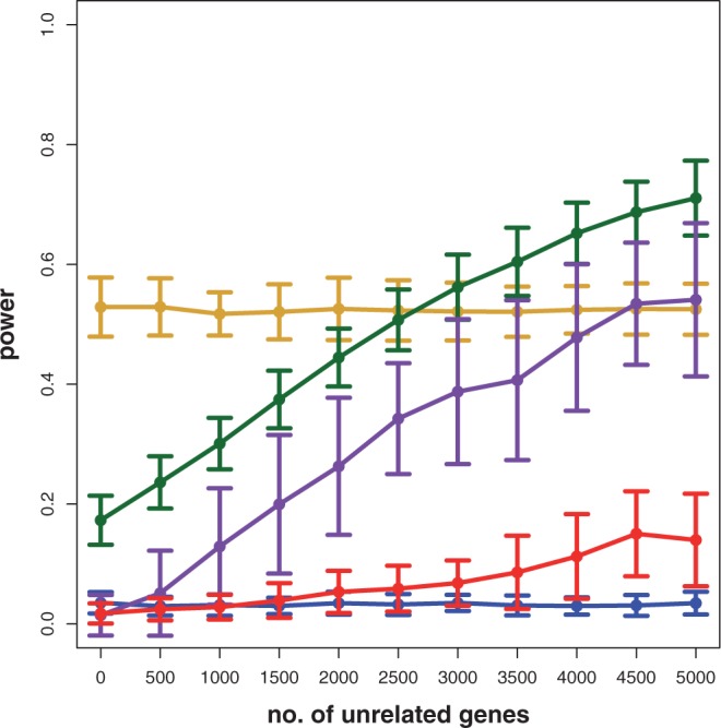
Results for simulated data. Estimated power for GSEA (red), GSA (blue), GSEArot (purple), GAGE (green) and random set (gold) in dependence on the number of additional genes in the background data set.

Interestingly, the POSP increases significantly for GAGE, GSEA and GSEArot by adding more genes in the analysis by using a less stringent filtering. In Figure 4, middle, we show the rescaled number of significant pathways of these three methods, which we call the POSP, obtained from the transformation,

(4)

Here, y(g) corresponds to the number of significant pathways for g genes and and to the minimum and maximum values of y(g), respectively. For the three methods, these parameters are shown in the Supplementary Table S1. For GSEA (red), GSEArot (purple) and GAGE (green), the POSP for g_M genes is between 0.03 and 0.80. Hence, using a less stringent filtering criterion allows in all three methods a significant gain in the POSP, depending on the data. An additional problem is given by the lack of control of the reference FDR, shown in Figure 4, right. On a note, because GSEA has an empty reference list of pathways for the prostate cancer data set, any significant pathway corresponds to a false negative. For this reason, the reference FDR is either one or not defined.

These examples allow a concrete description why such a behavior of a method is problematic. Usually, the IQR is used in the preprocessing step for microarray data to filter out genes that either are not expressed or for which the measurement is corrupted. However, our results demonstrated that exactly these genes with an IQR < (on the right-hand side of the dashed line) lead to an improvement of the power and the POSP. In other words, the addition of data that are potentially random improves the methods. Another problem that can be explained with the help of this example is that such methods are tempting for its users to apply either a larger IQR as suggested by the data or to not filter the data at all. Both choices result in similar consequences, namely, an increased power and a higher number of significant pathways, although the ‘additional’ data are potentially random.

Influence of the background: simulated data

To get a more refined view on the effects observed for the three cancer data sets, we repeat a similar analysis for simulated data. Specifically, we study the influence that ‘unrelated data’ in the background data, i.e. , have on the power of the competitive methods. For our simulations, we define 150 non-overlapping pathways, each consisting of 50 genes, and within each pathway, the average correlation between the genes is ρ = 0.1. This results in 7500 genes that are included in this data set. From these 150 pathways, we select randomly 100 pathways and change the mean expression values of 50% of the genes in these pathways. That means the detection call in these 100 pathways is 50%. We label these 100 pathways as ‘true positive’, and the remaining 50 pathways as ‘true negative’. These data constitute D^e. In addition, we include ‘unrelated’ genes that do not change their mean expression values between the treatment and control group. That means we add genes to the data set, which are not differentially expressed, and their expression values are sampled from the same distribution as for the non-differentially expressed genes, i.e. from N(0,1). The number of these unrelated genes corresponds to the x-axis in Figure 5. Because these unrelated genes do not belong to any of the 150 pathways, they contribute only to the background data.

In Figure 5, we show the estimated power of GSEA (red), GSA (blue), GSEArot (purple), GAGE (green) and ‘random set’ (gold), depending on the number of unrelated genes added to the data set. The number of unrelated genes ranges from 0 to 5000, in steps of 500 genes. That means the total number of genes in the extended data set ranges from 7500 to 12 500. From Figure 5, one can see that only the power of ‘random set’ (gold) and GSA (blue) is invariant with respect to the number of unrelated genes; hence, these methods exhibit a desirable behavior. All other methods increase their power by increasing the number of unrelated genes. GSEArot (purple) shows the highest raise in power by a factor of 17, followed by GAGE (green, 3.88) and GSEA (red, 3.33).

To emphasize the fundamental statistical problem with GAGE, GSEA and GSEArot, showing an increase in power when unrelated genes () are added to the analysis, we present the following argument. Suppose one conducts a two-sample t-test. For a given effect size Δμ (difference of sample mean values in the two samples), a power and a significance level α, one can estimate the sample size that is necessary to control the type I error at the desired significance level (36). For example, for an effect size of Δμ = 1, a power of 0.9 and α = 0.05, the required sample size is . Here it is important to realize that with the effect size, we define the anticipated ‘strength of the signal in the data’, and the obtained number of samples from the above calculation tells us that by using >22 samples, we can distinguish such a signal strength from noise. If, instead, the anticipated effect size (signal strength) would be Δμ = 0.01 (all other parameters unchanged), we need samples. Hence, the smaller the effect size (signal), the more samples are required to distinguish such a signal from noise. This behavior is intuitively plausible, as we assume that more samples imply more information in the data. We would like to highlight that a two-sample t-test is ‘self-contained’ in the sense that only the data from the two samples are used, but no background data (). Now, the crucial point is that ‘competitive’ gene set methods, namely GAGE, GSEA and GSEArot, do not behave this way. Instead, these methods improve ‘seemingly’ their power when ‘unrelated’ data, which do not contain information (), are added to the background data. The key to realize is that the unrelated genes in the background do not contain information but are essentially noise.

A serious implication of this is demonstrated in Figure 6. In this figure, we are testing just one pathway consisting of 100 genes, for a sample size of 10 (each condition). The expression values for the control group are sampled from N(0,1), and the expression values for the treatment group are sampled from , with μ = 0.09. These data constitute D^e. Furthermore, the expression values of the unrelated genes in the background data are sampled from N(0,1) (control and treatment). Each box plot in Figure 6 corresponds to a distribution of P-values resulting from 50 hypotheses’ tests from independent data sets. One can see that despite the small difference between the mean expression values of the treatment and control group (Δμ = 0.09), GAGE, GSEA and GSEArot declare this pathway as significant (for α = 0.05) if the number of unrelated genes in the background data is larger than a certain number. With respect to the median of the P-values, this threshold gene number is 1500, 100 and 100 (genes) for GAGE, GSEA and GSEArot, respectively. We would like to emphasize that the sample size remains fixed for all simulations, which implies that the amount of information in the data (D^e) is also fixed and does not increase by adding more unrelated genes () to the analysis.

Figure 6.

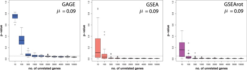
Distribution of P-values of one pathway with 100 genes, resulting from tests with GAGE (left), GSEA (middle) and GSEArot (right). The x-axis gives the number of unrelated genes in the background. For all simulations, the sample size is fixed.

The crucial point is that the size of the background (number of genes) of these competitive tests ‘assumes’ a similar role as the sample size for self-contained tests. This implies that GAGE, GSEA and GSEArot do not possess a sensitivity limit, as self-contained tests do. For any self-contained test, such a sensitivity limit is naturally given by the (complex) interplay between effect size and sample size. Instead, for the above competitive tests, including unrelated genes to the background can increase the sensitivity of these tests with respect to any effect size, even for a fixed sample size. Theoretically, this means that for any effect size and a sufficiently large number of unrelated genes in the background, any gene set could become significant whenever .

The problem is that the methods GAGE, GSEA and GSEArot cannot distinguish between D^e and D^u, as they are using the combined data set . Hence, they treat D^u implicitly as it would correspond to experimental data, containing actual information about an experiment. However, this can lead to false assessments because D^u allows controlling the strength of a signal by changing the data, resulting in a lack of a sensitivity limit.

In the supplementary file, we show additional simulation results for the POSP. As one can see in Supplementary Figure S1, these results reflect our findings for the biological data, shown in Figure 4 (middle column). From Supplementary Figure S1, one can see that with an increasing number of unrelated genes (g), also the POSP increases. This behavior is largely independent of the strength of the correlation. This observation confirms our finding discussed above that the sensitivity of these three competitive methods can be controlled by the number of unrelated genes, g, in the background because for a sufficiently large number of background genes, any pathway with can become significant. However, this makes statements like ‘a pathway with is truly null’ ill posed. Instead, one needs to refine such an assertion for GSEA, GSEArot and GAGE to obtain a precise statement:

SP1: Pathways with and a number of unrelated genes in the background are truly null with respect to a data set D^e.

If the information about the background data would not be included, this statement would be inexpressive because by increasing the number of unrelated genes in the background data , without changing the experimental data D^e or the effect size Δμ, it can be invalidated, as demonstrated in Supplementary Figure S1.

DISCUSSION

In this article, we investigated five common competitive gene sets methods with respect to the dependency of these methods on (i) the correlation structure in the data, (ii) the effect of up- and down-regulation of genes, (iii) the influence of the background data and (iv) the influence of the sample size. From studying the influence the correlation and the proportion of up-regulated genes have, we found that the power of ‘random set’ is most robust with respect to the presence of correlations in the data (see Figure 3). All other methods are much stronger affected, with GSEA performing least favorable. The reason why ‘random set’ is unaffected by sample-label permutations is that its test statistic, (see in supplementary file Equation 1), is based on individual gene statistics, which are invariant against sample-label permutations. These results are in contrast to the influence the proportion of up-regulated genes has on the power. For these data, we found GAGE to outperform all other methods.

From investigating the influence of the background data, we found that the methods GSEA, GSEArot, ‘random set’, GAGE and GSA can be categorized into two groups. In the first group are ‘random set’ and GSA, and in the second are GAGE, GSEA and GSEArot. For methods in the first group, we found no noticeable influence of the number of unrelated genes in the background data on the power, for simulated data and microarray data. However, methods in the second two are severely affected. These results are consistent for simulated and three cancer microarray data sets.

The conceptual understanding and the expectations we have of statistical methods is that these must not improve by adding ‘unrelated’ data to a given data set, as D^u does not contain information. Here, we used the term ‘unrelated’ because for real microarray data, it is not easy to decide whether a gene is not expressed at all or whether it merely has a low basal expression. As discussed in section ‘Influence of data filtering: ALL, prostate cancer and breast cancer’, with an increasing distance from the median filtering toward a less stringent filtering criterion, the tendency of genes to be truly expressed decreases. In this respect, the meaning of ‘unrelated’ converges to ‘random’. In contrast, for simulated data, genes behaving randomly are clearly defined. For this reason, we used the more neutral term ‘unrelated’, instead of ‘random’ or ‘noise’, to be applicable to both, simulated and biological data. In this respect, the behavior of the methods in the second group is undesirable, as it entails a temptation on the users to apply a less stringent filtering criterion to the data, hence leading to the pollution of a data set by ‘not excluding’ unrelated data. If GAGE, GSEA or GSEArot are used in combination with a data set that contains ‘unrelated’ data (), the obtained results become flawed. Here, it is important to distinguish between a flaw in a method itself and a deficient application, and we would like to emphasize that only the application of GAGE, GSEA and GSEArot in combination with ‘unrelated’ data makes the results flawed. If these methods are used with adequate data, the results are proper.

As shown by our analysis, the key problem of GAGE, GSEA and GSEArot is that the data D^u influence the significance of a pathway, whereas D^e remains unchanged. This is a logical contradiction because the unrelated data D^u do not contain information about the experiment. In other words, the reason for this curious behavior is that the data D^u, which do not contain information, are treated by the methods ‘as if’ they would contain information. In this way, D^u is not only polluting the background data but also the data of target pathways, as both may involve unrelated data (in the form of and ). As a consequence of the entering of D^u in the analysis, the difference between a signal and noise vanishes, implying a loss of a statistical sensitivity limit.

To avoid an improper usage of GAGE, GSEA and GSEArot, two points are crucial to consider. First, one needs to make sure that no data are included in the analysis that represent ‘unrelated’ data, i.e. D^u needs to be removed. For microarray data, this implies the application of a data filtering procedure aiming to remove all genes that do not have at least a basal expression level. Unfortunately, this is not sufficient, because also D^e plays a crucial role. Whereas it is in the hand of the analyst to make sure that D^u is (at least approximately) excluded from an analysis, it is impossible to ensure the second crucial point, namely, that the data set D^e is ‘complete’. This means one needs to use ‘all’ expression data from ‘all’ expressed genes in a genome to establish a meaningful definition of statistical significance. However, usually microarray chips contain only a subset of all genes from an organism. This implies that the available data set D^e is only a subset of the complete expression data set D^E of an organism; hence, pathways declared as significant for D^e may not be significant for the complete data set D^E or vice versa.

Based on our analysis, we are suggesting the following procedure for using GAGE, GSEA and GSEArot. For gene expression data from biological or biomedical experiments using a genome-scale microarray chip like the ‘Affymetrix Human Genome U133 Plus 2.0 Array’ for human or ‘Affymetrix Yeast Genome S98 Array’ for yeast, we suggest a stringent gene filtering removing all unrelated data from a given data set. This allows a meaningful analysis with a well-defined statistical interpretation of the obtained results. For all other non–genome-scale gene expression data sets, this is not necessarily guaranteed, and the severity of this deviation can only be answered in a case-by-case manner. For gene expression data from biomedical experiments or clinical studies, which do not provide genome-scale expression data for ‘all’ genes, we advise strongly against the application of GSEA, GSEArot or GAGE because of the unclear nature of the interpretation for the obtained results lying outside the realm of statistical inference.

In this context, RNA-seq data obtained from next-generation sequencing technologies have a clear conceptual advantage over DNA microarray chips because, principally, all mRNAs of an organism are sequenced, and hence, are available for analysis (37,38). This simplifies the experimental design for competitive gene set analysis methods considerably, as the requirement for the availability of all gene expression values for all genes in a genome is naturally fulfilled.

Our recommendations are in striking contrast to the recommended usage of GSEA given in (39): ‘The GSEA algorithm does not filter the expression dataset and does not benefit from your filtering of the expression dataset’. Furthermore, it is reported that the findings in (40) show that filtered and unfiltered data give the same results. Unfortunately, one particular example does not establish a legitimate usage for generic data set, as our results demonstrate. Following the above reference given in (39), thus far, many articles have been published under the impression that the usage of unfiltered data is not harmful (41). Based on our analysis, we recommend repeating each of these analyses to test the influence of the filtering explicitly.

CONCLUSION

In summary, our analysis revealed that when using competitive gene set methods, it is imperative to apply a stringent gene filtering criterion. However, even when the data are filtered appropriately, for gene expression data from chips that do not provide a genome-scale coverage of the expression values of all mRNAs, this is not enough for GSEA, GSEArot and GAGE to ensure the statistical soundness of the applied procedure. For this reason, for biomedical and clinical studies, we strongly advice not to use GSEA, GSEArot and GAGE for such data sets.

SUPPLEMENTARY DATA

Supplementary Data are available at NAR Online: Supplementary Tables 1 and 2 and Supplementary Figure 1.

FUNDING

Shailesh Tripathi is supported by a studentship from the National Institute of Immunology. Funding for open access charge: Waived by Oxford University Press.

Conflict of interest statement. None declared.

REFERENCES

- 1.von Bertalanffy L. The theory of open systems in physics and biology. Science. 1950;111:23–29. doi: 10.1126/science.111.2872.23. [DOI] [PubMed] [Google Scholar]
- 2.Barabási AL, Oltvai ZN. Network biology: understanding the cell's functional organization. Nat. Rev. 2004;5:101–113. doi: 10.1038/nrg1272. [DOI] [PubMed] [Google Scholar]
- 3.Emmert-Streib F, Dehmer M. Networks for systems biology: conceptual connection of data and function. IET Syst. Biol. 2011;5:185–207. doi: 10.1049/iet-syb.2010.0025. [DOI] [PubMed] [Google Scholar]
- 4.Niiranen S, Ribeiro A, editors. Information Processing and Biological Systems. Berlin: Springer; 2011. [Google Scholar]
- 5.Palsson B. Systems Biology. Cambridge; New York: Cambridge University Press; 2006. [Google Scholar]
- 6.Vidal M. A unifying view of 21st century systems biology. FEBS Lett. 2009;583:3891–3894. doi: 10.1016/j.febslet.2009.11.024. [DOI] [PubMed] [Google Scholar]
- 7.Zanzoni A, Soler-Lopez M, Aloy P. A network medicine approach to human disease. FEBS Lett. 2009;583:1759–1765. doi: 10.1016/j.febslet.2009.03.001. [DOI] [PubMed] [Google Scholar]
- 8.Mootha V, Lindgren C, Eriksson K, Subramanian A, Sihag S, Lehar J, Puigserver P, Carlsson E, Ridderstråle M, Laurila E, et al. PGC-1alpha-responsive genes involved in oxidative phosphorylation are coordinately downregulated in human diabetes. Nat. Genet. 2003;34:267–273. doi: 10.1038/ng1180. [DOI] [PubMed] [Google Scholar]
- 9.Emmert-Streib F, Glazko G. Pathway analysis of expression data: deciphering functional building blocks of complex diseases. PLoS Comput. Biol. 2011;7 doi: 10.1371/journal.pcbi.1002053. e1002053. [DOI] [PMC free article] [PubMed] [Google Scholar]
- 10.Ashburner M, Ball C, Blake J, Botstein D, Butler H, Cherry JM, Davis AP, Dolinski K, Dwight SS, Eppig JT, et al. Gene ontology: tool for the unification of biology. The Gene Ontology Consortium. Nat. Genet. 2000;25:25–29. doi: 10.1038/75556. [DOI] [PMC free article] [PubMed] [Google Scholar]
- 11.Subramanian A, Tamayo P, Mootha V, Mukherjee S, Ebert B, Gillette M, Paulovich A, Pomeroy S, Golub T, Lander E, et al. Gene set enrichment analysis: a knowledge-based approach for interpreting genome-wide expression profiles. Proc. Natl Acad. Sci. USA. 2005;102:15545–15550. doi: 10.1073/pnas.0506580102. [DOI] [PMC free article] [PubMed] [Google Scholar]
- 12.Kanehisa M, Goto S. KEGG: Kyoto encyclopedia of genes and genomes. Nuclei Acids Res. 2000;28:27–30. doi: 10.1093/nar/28.1.27. [DOI] [PMC free article] [PubMed] [Google Scholar]
- 13.Abatangelo L, Maglietta R, Distaso A, D’Addabbo A, Creanza T, Mukherjee S, Ancona N. Comparative study of gene set enrichment methods. BMC Bioinformatics. 2009;10:275. doi: 10.1186/1471-2105-10-275. [DOI] [PMC free article] [PubMed] [Google Scholar]
- 14.Emmert-Streib F. The chronic fatigue syndrome: a comparative pathway analysis. J. Comput. Biol. 2007;14: 961–972. doi: 10.1089/cmb.2007.0041. [DOI] [PubMed] [Google Scholar]
- 15.Glazko G, Emmert-Streib F. Unite and conquer: univariate and multivariate approaches for finding differentially expressed gene sets. Bioinformatics. 2009;25:2348–2354. doi: 10.1093/bioinformatics/btp406. [DOI] [PMC free article] [PubMed] [Google Scholar]
- 16.Irizarry RA, Wang C, Zhou Y, Speed TP. Gene set enrichment analysis made simple. Stat. Methods Med. Res. 2009;18:565–575. doi: 10.1177/0962280209351908. [DOI] [PMC free article] [PubMed] [Google Scholar]
- 17.Jung K, Becker B, Brunner E, Beißbarth T. Comparison of global tests for functional gene sets in two-group designs and selection of potentially effect-causing genes. Bioinformatics. 2011;27:1377–1383. doi: 10.1093/bioinformatics/btr152. [DOI] [PubMed] [Google Scholar]
- 18.Klebanov L, Glazko G, Salzman P, Yakovlev A, Xiao Y. A multivariate extension of the gene set enrichment analysis. J. Bioinform. Comput. Biol. 2007;5:1139–1153. doi: 10.1142/s0219720007003041. [DOI] [PubMed] [Google Scholar]
- 19.Nam D, Kim S. Gene-set approach for expression pattern analysis. Brief Bioinform. 2008;9:189–197. doi: 10.1093/bib/bbn001. [DOI] [PubMed] [Google Scholar]
- 20.Ackermann M, Strimmer K. A general modular framework for gene set enrichment analysis. BMC Bioinformatics. 2009;10:47. doi: 10.1186/1471-2105-10-47. [DOI] [PMC free article] [PubMed] [Google Scholar]
- 21.Goeman J, Buhlmann P. Analyzing gene expression data in terms of gene sets: methodological issues. Bioinformatics. 2007;23:980–987. doi: 10.1093/bioinformatics/btm051. [DOI] [PubMed] [Google Scholar]
- 22.Dørum G, Snipen L, Solheim M, Sæbø S. Rotation testing in gene set enrichment analysis for small direct comparison experiments. Stat. Appl. Genet. Mol. Biol. 2009;8 doi: 10.2202/1544-6115.1418. Article 34. [DOI] [PubMed] [Google Scholar]
- 23.Newton M, Quintana F, denBoon JA, Sengupta S, Ahlquist P. Random-set methods identify distinct aspects of the enrichment signal in gene-set analysis. Ann. Appl. Stat. 2007;1:85–106. [Google Scholar]
- 24.Luo W, Friedman M, Shedden K, Hankenson KD, Woolf PJ. GAGE: generally applicable gene set enrichment for pathway analysis. BMC Bioinformatics. 2009;10:161. doi: 10.1186/1471-2105-10-161. [DOI] [PMC free article] [PubMed] [Google Scholar]
- 25.Efron B, Tibshiran R. On testing the significance of sets of genes. Ann. Appl. Stat. 2007;1:107–129. [Google Scholar]
- 26.Ge Y, Dudoit S, Speed T. Resampling-based multiple testing for microarray data analysis. TEST. 2003;12:1–77. [Google Scholar]
- 27.Good P. Permutation, Parametric and Bootstrap Tests of Hypotheses. New York: Springer; 2005. [Google Scholar]
- 28.Singh D, Febbo PG, Ross K, Jackson DG, Manola J, Ladd C, Tamayo P, Renshaw AA, D’Amico A, Richie JP, et al. Gene expression correlates of clinical prostate cancer behavior. Cancer Cell. 2002;1:203–209. doi: 10.1016/s1535-6108(02)00030-2. [DOI] [PubMed] [Google Scholar]
- 29.Nam D. De-correlating expression in gene-set analysis. Bioinformatics. 2010;26:i511–i516. doi: 10.1093/bioinformatics/btq380. [DOI] [PMC free article] [PubMed] [Google Scholar]
- 30.Chiaretti S, Li X, Gentleman R, Vitale A, Wang KS, Mandelli F, Foa R, Ritz J. Gene expression profiles of B-lineage adult acute lymphocytic leukemia reveal genetic patterns that identify lineage derivation and distinct mechanisms of transformation. Clin. Cancer Res. 2005;11:7209–7219. doi: 10.1158/1078-0432.CCR-04-2165. [DOI] [PubMed] [Google Scholar]
- 31.Miller LD, Smeds J, George J, Vega VB, Vergara L, Ploner A, Pawitan Y, Hall P, Klaar S, Liu ET, et al. An expression signature for p53 status in human breast cancer predicts mutation status, transcriptional effects, and patient survival. Proc. Natl Acad. Sci. USA. 2005;102:13550–13555. doi: 10.1073/pnas.0506230102. [DOI] [PMC free article] [PubMed] [Google Scholar]
- 32.Hahne F, Huber W, Gentleman R, Falcon S. Bioconductor Case Studies. New York, NY: Springer; 2008. [Google Scholar]
- 33.Bourgon R, Gentleman R, Huber W. Independent filtering increases detection power for high-throughput experiments. Proc. Natl Acad. Sci. USA. 2010;107:9546–9551. doi: 10.1073/pnas.0914005107. [DOI] [PMC free article] [PubMed] [Google Scholar]
- 34.Draghici S, Khatri P, Eklund AC, Szallasi Z. Reliability and reproducibility issues in DNA microarray measurements. Trends Genet. 2006;22:101–109. doi: 10.1016/j.tig.2005.12.005. [DOI] [PMC free article] [PubMed] [Google Scholar]
- 35.Benjamini Y, Hochberg Y. Controlling the false discovery rate: a practical and powerful approach to multiple testing. J. R. Stat. Soc. Ser. B (Methodological) 1995;57:125–133. [Google Scholar]
- 36.Cohen J. Statistical Power Analysis for the Behavioral Sciences. NJ: Number 1990 Erlbaum, Hillsdale; 1988. [Google Scholar]
- 37.Marguerat S, Bähler J. RNA-seq: from technology to biology. Cell. Mol. Life Sci. 2010;67:569–579. doi: 10.1007/s00018-009-0180-6. [DOI] [PMC free article] [PubMed] [Google Scholar]
- 38.Wang Z, Gerstein M, Snyder M. RNA-Seq: a revolutionary tool for transcriptomics. Nat. Rev. Genet. 2009;10:57–63. doi: 10.1038/nrg2484. [DOI] [PMC free article] [PubMed] [Google Scholar]
- 39.GSEA team GSEA User Guide v3.82 The Broad Institute Boston, USA. (2011) http://www.broadinstitute.org/gsea/doc/GSEAUserGuideFrame.html. [Google Scholar]
- 40.Monti S, Savage KJ, Kutok JL, Feuerhake F, Kurtin P, Mihm M, Wu B, Pasqualucci L, Neuberg D, Aguiar RCT, et al. Molecular profiling of diffuse large B-cell lymphoma identifies robust subtypes including one characterized by host inflammatory response. Blood. 2005;105:1851–1861. doi: 10.1182/blood-2004-07-2947. [DOI] [PubMed] [Google Scholar]
- 41.Huang DW, Sherman BT, Lempicki RA. Bioinformatics enrichment tools: paths toward the comprehensive functional analysis of large gene lists. Nucleic Acids Res. 2009;37:1–13. doi: 10.1093/nar/gkn923. [DOI] [PMC free article] [PubMed] [Google Scholar]
Associated Data
This section collects any data citations, data availability statements, or supplementary materials included in this article.