Characterization of Ambient Air Pollution Measurement Error in a Time-Series Health Study using a Geostatistical Simulation Approach

Abstract

In recent years, geostatistical modeling has been used to inform air pollution health studies. In this study, distributions of daily ambient concentrations were modeled over space and time for 12 air pollutants. Simulated pollutant fields were produced for a 6-year time period over the 20-county metropolitan Atlanta area using the Stanford Geostatistical Modeling Software (SGeMS). These simulations incorporate the temporal and spatial autocorrelation structure of ambient pollutants, as well as season and day-of-week temporal and spatial trends; these fields were considered to be the true ambient pollutant fields for the purposes of the simulations that followed. Simulated monitor data at the locations of actual monitors were then generated that contain error representative of instrument imprecision. From the simulated monitor data, four exposure metrics were calculated: central monitor and unweighted, population-weighted, and area-weighted averages. For each metric, the amount and type of error relative to the simulated pollutant fields are characterized and the impact of error on an epidemiologic time-series analysis is predicted. The amount of error, as indicated by a lack of spatial autocorrelation, is greater for primary pollutants than for secondary pollutants and is only moderately reduced by averaging across monitors; more error will result in less statistical power in the epidemiologic analysis. The type of error, as indicated by the correlations of error with the monitor data and with the true ambient concentration, varies with exposure metric, with error in the central monitor metric more of the classical type (i.e., independent of the monitor data) and error in the spatial average metrics more of the Berkson type (i.e., independent of the true ambient concentration). Error type will affect the bias in the health risk estimate, with bias toward the null and away from the null predicted depending on the exposure metric; population-weighting yielded the least bias.

1. Introduction

Understanding measurement error impacts in studies of ambient air pollution and health is challenging due to the use of group-level exposure measures derived from monitor data to infer the adverse health effects of air pollution on the individual level. Moreover, the true ambient air pollution level is not known. Here, we address measurement error in a time-series analysis that utilizes health outcomes aggregated over a geographical area, with the true unobserved exposure defined as the regulatory ambient concentration at individual residences.

Measurement error is inherent in time-series epidemiologic studies of air pollution that rely on ambient monitor data. Instrument error and, to a greater degree, exposure misclassification due to the spatial variability have been shown to bias effect estimates in large population studies (Chen et al., 2007; Goldman et al., 2010; Sarnat et al., 2010; Wilson et al., 2007). Time-series studies that rely on central monitor data have been criticized for uncertainty related to exposure measurement errors and the substantial variation present in some air pollutant measures (Dominici et al., 2006). Both error amount and error type affect health risk estimates and statistical power. An increase in the amount of error decreases the statistical power to detect health associations (e.g., Goldman et al., 2011). Error type (e.g., classical and Berkson) has been demonstrated to modify the extent to which measurement error attenuates health effect estimates (Armstrong, 1998; Goldman et al., 2011; Sheppard et al., 2005; Zeger et al., 2000). Classical error is that in which the measurement varies randomly about the true exposure. In contrast, with Berkson error the true exposure varies randomly about the measurement, such as might be the case if an average of individual exposures across the at-risk population is used to characterize ambient exposure. Purely Berkson error is expected to decrease significance of an association but will yield an unbiased effect estimate (Armstrong, 1998; Zeger et al., 2000). Because the distribution of true concentrations cannot be known with certainty, assessment of error type for a given dataset is challenging.

Increasingly, advanced spatial modeling techniques are being employed to gain insight on the distribution of true ambient concentrations (Jerrett et al., 2010). Several studies have developed methods for simulating air pollutant concentrations, taking into account both spatial and temporal characteristics of concentrations (Nunes and Soares, 2005; Sahu and Mardia, 2005); however, few studies have used such simulations to assess the amount and type of measurement error in time-series studies (Peng and Bell, 2010). Gryparis and coauthors (2009) used a smoothing method of spatial measurement error modeling to explore the relative uncertainties associated with use of different exposure metrics in a study of particulate matter (PM) and birth weight in greater Boston. Fuentes et al. (2006) utilized multivariate regression to model the spatial structure of concentrations in order to quantify uncertainties in an association between mortality and fine PM. Peng and Bell (2010) estimated county-wide average concentrations to assess spatial misalignment error and apply statistical methods to obtain adjusted health risk estimates in a time-series study of PM components and hospital admissions for cardiovascular disease. Lee and Shaddick (2010) jointly modeled pollutant concentrations and health data using a Bayesian spatio-temporal model and found that pollution surface modeling may provide better health effect estimates in areas where a large number of monitoring sites are available, particularly for more spatially varying species.

In previous work, we found instrument error and the lack of spatial autocorrelation of ambient pollutant concentrations can lead to substantial reduction in statistical power and potential attenuation of risk estimates (Goldman et al., 2010), with error type affecting the amount of attenuation (Goldman et al., 2011). Our previous studies did not, however, characterize the type of error actually present in ambient measurements or account for the spatial heterogeneity in pollution levels. Moreover, while there has been substantial discussion of the potential impact of error type, few studies have attempted to determine the error type of air pollutant monitoring data in a time-series setting. To do this, the relationship between the true ambient concentration and the measured ambient concentration used in the health study should be understood and quantified. Receptor-based approaches for assessing this relationship require detailed spatial and temporal observations that are not typically available from ambient monitoring networks. Emissions-based models of ambient air pollution, such as the Community Multi-scale Air Quality (CMAQ) modeling system, observation-based interpolation methods, such as kriging (Mulholland et al., 1998), and hybrids of these methods (Kaynak et al., 2009; Mendoza-Dominguez and Russell, 2001) are able to capture many characteristics of ambient concentrations at high spatial and temporal resolution; however, they fail to describe the low spatial dependence for some pollutants that is evident from observational data. This is particularly relevant to assessing error in time-series studies where monitors placed using criteria that do not necessarily maximize representativeness are used to derive population average exposure. In this work, we use geostatistical methods to create simulated ambient air pollution fields that have the desired spatial and temporal distribution properties found in actual ambient monitor data for 12 air pollutants. For each pollutant time-series, six properties were modeled: temporal autocorrelation, spatial autocorrelation, mean, standard deviation, seasonal trend, and day-of-week trend. Using these “true” ambient air pollution fields, monitor data are simulated that incorporate instrument imprecision as classical error. Next, the amount and type of measurement error present in using alternative time-series exposure metrics (i.e., central monitor data and various monitor averages) to represent ambient air pollutant levels over time and space is assessed. Finally, the impact of measurement error on health risk estimates is predicted.

This work addresses measurement error with respect to the assessment of health risk associated with ambient air pollution using a time-series study design and regulatory air pollution monitors. This work does not address near-source variability in ambient air pollution, such as near roadways, or variability in personal exposure.

2. Methods

2.1 Air Quality Data

To assess spatio-temporal trends in air pollutant concentrations, daily measures of ambient monitor data for the 20-county study area for a 6-year period (1999–2004) were analyzed for 12 ambient air pollutants: 1-hr max NO₂, 1-hr max NO_x, 8-hr max O₃, 1-hr max SO₂, 1-hr max CO, 24-hr PM₁₀ mass, 24-hr PM_2.5 mass, and 24-hr PM_2.5 components sulfate (SO₄²⁻), nitrate (NO₃⁻), ammonium (NH₄⁺), elemental carbon (EC) and organic carbon (OC). Data were obtained from three monitoring networks: the US EPA’s Air Quality System (AQS), including State and Local Air Monitoring System and Speciation Trends Network for PM_2.5 component measurements; the Southeastern Aerosol Research and Characterization Study (SEARCH) network (Hansen et al., 2003), including the Atlanta EPA supersite at Jefferson Street (Solomon et al., 2003); and the Assessment of Spatial Aerosol Composition in Atlanta (ASACA) network (Butler et al., 2003). While some differences exist between measurement methods used by the monitoring networks, these discrepancies have been discussed in detail elsewhere (Goldman et al., 2010) and are expected to have a negligible impact on this analysis.

Monitor site locations are shown in Figure 1. Data from six NO₂/NO_x monitors, five CO monitors, five SO₂ monitors, five O₃ monitors, eight PM₁₀ monitors, nine PM_2.5 monitors, and five speciated PM_2.5 monitors were used. The following distributional features of the pollutant fields were characterized: temporal autocorrelation, spatial autocorrelation, and mean, standard deviation, seasonal trend, and day-of-week trend as functions of distance from the urban center.

Figure 1.

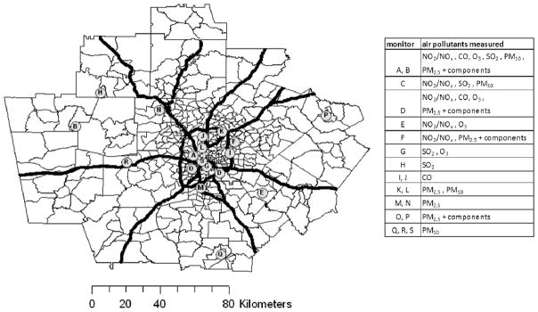
Map of the 20-county metropolitan Atlanta study area. Census tracts, expressways, and ambient air pollutant monitoring sites are shown. The urban center was defined at the intersection of expressways near the monitor labeled S, and the central monitor was defined as monitor A, the EPA supersite location.

2.2 Characterization of Air Pollutant Temporal and Spatial Distributions

Short-term temporal autocorrelation is present in daily ambient air pollutant data due to meteorological events occurring on time-scales of days to weeks. Correlations of data from each monitor were calculated for one to fourteen day lags (see Supplemental Material, Figure S.1 for central monitor results). The temporal autocorrelation trend with increasing lag was similar for urban, suburban and rural monitors, so short-term temporal autocorrelation was characterized as being independent of location. Across the 12 pollutants studied, means and standard deviations of the one-day and two-day lag Pearson correlation coefficients were 0.59 ± 0.13 and 0.33 ± 0.17, respectively. Secondary pollutants tend to have greater levels of short-term temporal autocorrelation that persists over longer lag periods.

Spatial autocorrelation depends on the distribution of emission sources and transport phenomena. Correlograms were constructed for each pollutant using data from all monitor pairs (Supplemental Material, Figure S.2). Primary pollutants, i.e., those largely emitted directly to the atmosphere such as NO_x, CO, SO₂ and EC, have much less spatial autocorrelation than secondary pollutants, i.e., those largely formed in the atmosphere such as O₃, NO₃⁻ and SO₄²⁻. Pollutants of mixed origin, e.g., PM_2.5 total mass and OC, have intermediate levels of spatial autocorrelation. Isotropic exponential models of the correlograms were developed, with the correlation coefficient at distance zero based on collocated instrument data. To estimate an average spatial autocorrelation for the study population, the correlogram for each pollutant was modeled as a function of distance from the urban center, correlation coefficients at 660 census tract centroids were estimated using this model, and these values were population-weighted and averaged by eq. 1 using 2000 census population data (Goldman et al., 2010).

$$\overline{R}=\frac{1}{P_{\mathit{total}}}\left(\sum _{j=1}^{660}{R}_j{P}_j\right)$$ (1)

Here, R_j is the Pearson correlation coefficient and P_j is the population at census tract j. Values of R̄ ranged from 0.90 for O₃ to 0.21 for SO₂ (Supplemental Material, Table S.1).

Air pollutant monitor data tend to have a lognormal distribution. Log means and log standard deviations are shown versus distance from the urban center in Supplemental Material, Figures S.3 and S.4, respectively. Ambient concentrations of pollutants predominantly from mobile sources (NO₂, NO_x, CO, and EC) decrease with increasing distance from the urban center. Pollutants largely of secondary origin, such as O₃ and PM_2.5 mass, tend to be relatively spatially homogeneous. The mean and standard deviation of air pollutant log concentrations were modeled as linear functions of distance from the urban center to 60 km; beyond 60 km these values were fixed at rural background levels.

Day-of-week and seasonal trends in air pollutant concentrations are shown in Supplemental Material, Figures S.5 and S.6, respectively. These trends result from variation in emissions by day-of-week and from variation in meteorology that affects mixing rates as well as formation and removal rates by season. Day-of-week trends were found to be similar at different monitor locations; these were modeled categorically. Seasonal trends were modeled using fourth-order polynomial functions under the constraints that the value and slope on the first day of each year are the same. Seasonal trends were found to differ between monitors in urban, suburban, and rural locations; therefore, fitted coefficients were varied with distance up to 60 km.

2.3 Simulation of Ambient Pollutant Fields

Daily air pollutant fields were generated for the 20-county Atlanta region (16,000 km²) at a 5-km resolution for a 6-year period (2,192 days) for the 12 ambient air pollutants. Additionally, 10 independent sets of simulations of daily CO fields were produced to assess the amount of numerical noise in this approach. These fields do not simulate actual ambient pollutant concentrations on any given day, but simulate air pollution over time and space for a population of days based on the characteristics described above. Simulations were produced via a two-step process. First, the direct sequential simulation method (Soares, 2001) in the Stanford Geostatistical Modeling Software (SGeMS) (Remy, 2005) was used to generate normalized fields (eq. 2) with the desired short-term temporal and spatial autocorrelation.

$${\chi }_{ij}^{\ast }=\frac{ln{C}_{ij}-{\mu }_{ln{C}_j}}{{\sigma }_{ln{C}_j}}~\text{N}(0,1)$$ (2)

Here, ${\chi }_{ij}^{\ast }$ is the normalized “true” pollutant level on day i at location j, C_ij is the concentration on day i at location j, μ_lnCj is the log concentration mean over all days at location j (Supplemental Material, Figure S.3), and σ_lnCj is the log concentration standard deviation over all days at location j (Supplemental Material, Figure S.4). Thus, at each location j, ${\chi }_{ij}^{\ast }$ has a mean of zero and a standard deviation of one. SGeMS was used in this application to provide spatial autocorrelation in two dimensions and temporal autocorrelation in a third dimension.

The second step in generating pollutant field simulations was denormalization to yield concentration fields with the desired means, standard deviations, day-of-week trends, and seasonal trends. This was achieved by inverting eq. 2 and applying factors to achieve the desired day-of-week and seasonal trends (eq. 3).

$$Z_{ij}^{\ast }={\alpha }_{wk}{\alpha }_{yr}exp\left({\chi }_{ij}^{\ast }{\sigma }_r+{\mu }_r\right)$$ (3)

Here, $Z_{ij}^{\ast }$ is the “true” concentration on day i at location j, μ_r is the log concentration mean modeled as a linear function of distance from urban center r, σ_r is the log concentration standard deviation modeled as a linear function of r, α_wk is the day-of-week factor modeled independent of r, and α_yr is the season factor modeled as a fourth-order polynomial function of r. Steps 1 and 2 were iterated in order to preserve the spatial and temporal autocorrelation structure observed in the monitor data (see Supplemental Material, Figures S1 and S2) after the simulated concentrations were denormalized and distribution trends were added. The final parameters μ_r, σ_r, α_wk, and α_yr used to simulate spatial trends in the mean and standard deviation and temporal trends by day-of-week and by season, respectively, are provided in Tables S.2 through S.4.

2.4 Simulation of Monitor Data and Calculation of Exposure Metrics

To simulate measurements at actual monitor site locations, classical instrument error was introduced to the simulated true values such that the Pearson correlation coefficient between the simulated monitor data (Z) and simulated true ambient (Z^*) equaled the square root of the correlation between actual collocated instrument data (Z₁ and Z₂ ); i.e., $R(Z,Z^{\ast })=\sqrt{R(Z_1,Z_2)}$ (Goldman et al., 2010). The simulated monitor data were then used to compute the following exposure metrics: central monitor and unweighted average, population-weighted average and area-weighted average of monitor data. The simulated Jefferson Street monitor time-series was defined as the central monitor exposure metric. A time-series of the unweighted average of simulated monitor data for each pollutant was computed as a second exposure metric. A population-weighted average time-series was computed from the simulated monitor data using census tract population from the 2000 census and a previously developed spatial interpolation method (Ivy et al., 2008). Lastly, an area-weighted average was computed using spatially interpolated simulated monitor data and census tract areas. These four time-series represent different exposure metrics that have been used in time-series epidemiologic studies to characterize population exposure.

Measurement error, ε_ij, was calculated for each exposure metric on each day i at each location in space j as the difference between the simulated exposure metric (Z_i), which is only a function of time, and the simulated true ambient concentration ( $Z_{ij}^{\ast }$), which is a function of both time and space: ${\epsilon }_{ij}=Z_i-Z_{ij}^{\ast }$. Population-weighted Pearson correlation coefficients were computed between ε_ij and the “measured” time-series (Z_i) and between ε_ij and the “true” concentrations ( $Z_{ij}^{\ast }$) by first calculating correlation coefficients over time at the 660 census tract centroids and then weighting each coefficient by eq. 1. For Berkson error, the expected value of $\overline{R_j({\epsilon }_{ij},Z_{ij}^{\ast })}$ is zero, whereas for classical error the expected value of $\overline{R_j({\epsilon }_{ij},Z_i)}$ is zero. In the subsequent presentation of results, subscripts denoting time and space and overbars denoting population-weighted averages are omitted for simplicity of presentation.

Finally, an expected amount of bias in the risk ratio estimate due to measurement error for each pollutant was calculated as the population-weighted slope of ε_ij versus Z_i based on our previous findings (Goldman et al., 2011). In epidemiologic time-series studies, Poisson regression models are often used to estimate risk ratios and confidence intervals for health effects associated with exposures. Here the risk ratio is the estimate of the proportional increase in the daily count of health outcomes, after controlling for potential confounding variables, associated with a given increase in exposure. In a large population epidemiologic study, there is error in the exposure estimate due to spatial variability that can bias the risk ratio estimate as well as reduce the statistical power to detect an effect of pollution.

3. Results

3.1 Comparison of Ambient Monitor Data and Ambient Field Simulations

Simulation results are provided in Supplemental Material in parallel with the presentation of observational data for the six features observed in monitor data described previously: short-term temporal autocorrelation (Figure S.8 simulation; Figure S.1 observation), spatial autocorrelation (Figure S.9 and Table S.5 simulation; Figure S.2 and Table S.1 observation), mean (Figure S.10 simulation; Figure S.3 observation), standard deviation (Figure S.11 simulation; Figure S.4 observation), day-of-week trend (Figure S.12 simulation; Figure S.5 observation), and seasonal trend (Figures S.13 and S.14 simulation; Figures S.6 and S.7 observation). Spatial trends in the mean and standard deviation and temporal trends by day-of-week and by season are well simulated by the denormalization parameters used in eq. 2 (μ_r, σ_r, α_wk, and α_yr, respectively). Observed and simulated short-term temporal autocorrelation and spatial autocorrelation are compared below; simulation of these features is essential to the evaluation of measurement error in this study, requiring the use of SGeMS.

Only small differences in short-term temporal autocorrelation (lags up to 14 days) were observed between urban and rural monitors; therefore, short-term temporal autocorrelation was modeled as independent of distance from the urban center. Observed and simulated short-term temporal autocorrelation trends are compared at the central monitoring site (Figure 2). The simulations capture the observed lower short-term autocorrelation of primary pollutants, such as NO_x, SO₂, CO and EC, relative to secondary pollutants, such as O₃, SO₄²⁻ and NO₃⁻.

Figure 2.

Short term temporal autocorrelation of measurements (black) and of the simulated time-series (gray) at the central monitoring site.

Spatial autocorrelation, as characterized by correlograms, is well captured by the simulations (Figure 3). The observed autocorrelation at distance zero is based on collocated instrument data, whereas the simulated true ambient autocorrelation goes to one as distance approaches zero. Instrument error is included by simulating monitor data, as described next.

Figure 3.

Spatial correlogram from monitoring site data (black line represents regression model result) and from simulated time-series results (gray points).

3.2 Exposure Metric Simulation

Time-series monitor data were simulated at actual monitor locations by introducing instrument error, consistent in amount with that of collocated instrument data for each pollutant and consistent in type with that of classical error on a log basis. Four alternative exposure metrics were derived from the simulated monitor data: central monitor, unweighted monitor average, population-weighted monitor average, and area-weighted monitor average. Means and standard deviations for these four time-series, as well as for the true population-weighted average calculated from the true ambient fields, are provided in Table 1. For primary pollutants, the central monitor means and standard deviations are much higher, and the area-weighted average values are lower, than those of other metrics, as expected, due to the averaging of heterogeneous pollutant fields. Also as expected, the monitor-based population-weighted metric has a mean and standard deviation most similar to the true population-weighted average; differences are largely due to the limited number and location of monitors. The unweighted average means and standard deviations tend to be most similar to the population-weighted average values, indicative of the fact that more monitors are located in areas of high population density.

Table 1.

Means and standard deviations over a six-year period of different exposure metrics calculated from simulated monitor data central monitor (CM), unweighted average (UA), population-weighted average (PWA), and area-weighted average (AWA) and of the true population-weighted average (TPWA) calculated from the simulated true ambient concentration field. Standard deviations for results of 10 independent sets of CO simulations are shown.

pollutant	CM		UA		PWA		AWA		TPWA
	mean	st dev	mean	st dev	mean	st dev	mean	st dev	mean	st dev
NO2 (ppb)	44.5	20.3	29.4	12.6	23.5	11.5	15.4	8.8	24.7	10.4
NOx (ppm)	0.117	0.118	0.065	0.057	0.046	0.041	0.025	0.021	0.052	0.042
CO (ppm)	1.58 ± 0.02	1.31 ± 0.06	1.07 ± 0.02	0.69 ± 0.04	0.75 ± 0.01	0.42 ± 0.02	0.45 ± 0.01	0.20 ± 0.01	0.72 ± 0.03	0.34 ± 0.04
SO2 (ppb)	14.0	22.8	12.8	12.3	10.3	10.6	8.9	7.9	12.2	8.56
O3 (ppb)	44.9	27.9	44.8	23.0	43.9	23.0	44.1	20.0	44.6	24.6
PM10 (μg/m3)	25.1	14.9	24.0	13.1	22.6	13.1	21.2	12.5	23.0	12.4
PM2.5 (μg/m3)	18.0	10.0	17.0	8.9	16.1	8.9	11.0	8.9	16.1	8.49
SO42− (μg/m3)	5.35	5.29	5.03	4.67	4.93	4.71	4.67	4.33	4.96	4.54
NO3− (μg/m3)	1.34	1.56	1.15	1.23	1.11	1.19	1.01	1.07	1.13	1.18
NH4+ (μg/m3)	2.32	1.85	2.34	1.72	2.24	1.72	2.22	1.64	2.30	1.70
EC (μg/m3)	0.90	0.88	0.70	0.54	0.62	0.49	0.50	0.38	0.68	0.50
OC (μg/m3)	5.93	4.29	5.33	3.31	5.10	3.28	4.69	2.90	5.16	3.15

3.3 Exposure Metric Evaluation of Error Type and Amount

Having produced simulated true air pollution fields and, from these fields, simulated monitor data and exposure metrics, we now address the type and amount of error present in each of the metrics for each pollutant. To assess the amount of numerical noise present, 10 independent sets of simulations of daily CO fields were produced. Standard deviations of results using these 10 simulations, shown in the figures and tables that follow, demonstrate that numerical noise impacts are small relative measurement error impacts.

As an indicator of error type, we calculate population-weighted Pearson correlation coefficients between error (ε= Z − Z^*) and Z^*, the “true” ambient concentration, and also between error and Z, the “measured” ambient concentration; results are shown in Table 2 for the four exposure metrics, as well as for the true population-weighted average. A zero value of R(ε,Z^*) suggests classical error, i.e., error independent of the true value; a zero value of R(ε,Z) suggests Berkson error, i.e., error independent of the measured value.

Table 2.

Population-weighted correlations between measurement error and true values, R(ε,Z^*), and between measurement error and measured values, R(ε,Z), where the true values, Z^*, are the true ambient concentration fields and the measured values, Z, are the monitor-based metrics of central monitor (CM), unweighted average (UA), population-weighted average (PWA), and area-weighted average (AWA) and the true population-weighted average (TPWA). Standard deviations of the correlations for 10 independent sets of CO simulations are shown.

pollutant	CM		UA		PWA		AWA		TPWA
	R(ε,Z*)	R(ε,Z)	R(ε,Z*)	R(ε,Z)	R(ε,Z*)	R(ε,Z)	R(ε,Z*)	R(ε,Z)	R(ε,Z*)	R(ε,Z)
NO2	−0.46	0.61	−0.73	0.20	−0.78	0.14	−0.87	−0.04	−0.82	0.0017
NO x	−0.11	0.81	−0.63	0.29	−0.81	0.02	−0.96	−0.31	−0.80	−0.00042
CO	−0.09 ± 0.02	0.86 ± 0.02	−0.48 ± 0.03	0.53 ± 0.04	−0.78 ± 0.02	0.17 ± 0.05	−0.99 ± 0.004	−0.21 ± 0.04	−0.86 ± 0.015	0.0016 ± 0.000045
SO2	−0.40	0.74	−0.73	0.35	−0.79	0.25	−0.88	0.08	−0.86	−0.0003
O3	0.03	0.39	−0.2	0.11	−0.21	0.11	−0.25	0.07	−0.28	−0.0006
PM10	−0.32	0.40	−0.43	0.15	−0.44	0.14	−0.51	0.07	−0.51	0.00039
PM2.5	−0.10	0.41	−0.28	0.14	−0.28	0.14	−0.29	0.13	−0.38	0.00065
SO42−	−0.05	0.41	−0.27	0.10	−0.25	0.12	−0.45	−0.09	−0.34	−0.00035
NO3−	0.08	0.58	−0.31	0.13	−0.38	0.05	−0.57	−0.16	−0.40	0.0022
NH4+	−0.37	0.28	−0.45	0.06	−0.45	0.07	−0.51	−0.02	−0.46	−0.00027
EC	−0.28	0.64	−0.65	0.14	−0.71	0.06	−0.85	−0.17	−0.70	−0.00007
OC	−0.18	0.54	−0.45	0.13	−0.46	0.12	−0.62	−0.07	−0.51	0.00007

The true population-weighted average, that is, the population-weighted average of the true ambient concentration at all locations, has error of the Berkson type, as expected, as evidenced by its near-zero values of R(ε,Z) (Table 2). This type of error would result in no bias in the health effect estimate. However, because the ambient concentration is measured imperfectly and at a limited number of locations, the error type when using the monitor-based metrics is not Berkson (i.e., R(ε,Z) ≠ 0) or classical (i.e., R(ε,Z^*) ≠ 0). The results in Table 2 suggest that errors associated with use of the different monitor averages are similar and perhaps more Berkson than classical, and errors associated with use of central monitor data are more classical-like than errors associated with use of monitor averages.

As an indicator of the amount of measurement error, we calculate the population-weighted correlation between measured exposure metric values and the true concentrations (Figure 4). The greater the measurement error, the lower this correlation and the less representative of population exposure is the measured exposure. In a time-series air pollution health effects study, a lower correlation reduces the power to detect a given association. As expected, primary pollutants such as CO, NO₂, NO_x, SO₂ and EC have lower correlations than secondary pollutants such as O₃, SO₄²⁻, and NO₃⁻, indicative of greater measurement error. Also as expected, central monitor data on average are less correlated with the true ambient exposure than monitor average data. Interestingly, there is little difference between using an unweighted average of monitor data or using a population-weighted average, likely due to the fact that there are few monitors for each pollutant and these tend to be located in more populated areas. Finally, it is noted that the population-weighted correlation between the true population-weighted average and the true ambient concentration is only slightly higher than the population-weighted correlation between the monitor averages and the true ambient concentration. This suggests that the amount of error is largely due to the use of a single metric to characterize exposure for a population for which there is spatial variability in the exposure. Nonetheless, while the amount of error, as indicated by the population-weighted average correlation between measured ambient concentration and true ambient concentration (Figure 4), is similar across monitor-based average metrics, the type of error, as indicated by the population-weighted correlation between error and the measured and true ambient concentrations (Table 2), varies across metrics.

Figure 4.

Population-weighted R² values between the true ambient concentration field and different exposure metrics, R²(Z,Z^*), where the exposure metrics are the monitor-based metrics of central monitor (CM), unweighted average (UA), population-weighted average (PWA) and area-weighted average (AWA), as well as the true population-weighted average (TPWA). Standard deviations of 10 sets of CO simulations are shown.

4. Discussion

Having used the simulation results to assess error type (Table 2) and amount (Figure 4) in four monitor-based exposure metrics, potential impacts of measurement error on bias and reduced statistical power in health risk estimates are discussed. Error type, as indicated by the correlation between error and the measured and true exposure (i.e., R(ε,Z) and R(ε,Z^*), respectively), is expected to affect the bias in the health risk estimate whereas error amount, as indicated by a lack of correlation between the measured exposure and the true exposure (i.e., R(Z,Z^*) < 1), is expected to reduce statistical power in the health risk estimate.

In previous work, we showed that the regressed slope, m, of measurement error (Z-Z^*) versus measurement (Z) is a good predictor of bias in the health risk estimate, such that m is approximately equal to the attenuation in risk ratio per unit where the fractional attenuation is defined as one minus the ratio of the health risk estimate based on measured exposure to the health risk estimate based on true exposure (Goldman et al., 2011). Therefore, we calculate a population-weighted value of m for each exposure metric and each pollutant (Figure 5). Risk ratio bias is predicted to be higher for primary pollutants (CO, SO₂, NO₂, NO_x, and EC) than for secondary pollutants (O₃, NO₃⁻, SO₄²⁻, and NH₄⁺). Use of the population-weighted average yields the least predicted bias (i.e., m nearest zero). Predicted bias-to-null is greatest when central monitor data are used as the exposure metric (i.e., largest m), whereas a bias away from the null (i.e., negative m) is predicted for use of the area-weighted average. The low variance of ambient pollution in less densely populated regions of the study area results in the low variation of the area-weighted average as compared to that of the true population-weighted average; thus, an observed association (i.e., observed change in health outcomes for a population per change in average exposure) will be greater (bias away from null) if the area-weighted average is used due to the underestimated change in exposure. In Figure 6, predicted bias, m, is shown across all pollutants and exposure metrics to be approximated as one minus the ratio of the true population-weighted average standard deviation to the measured exposure time-series standard deviation. These findings rely on the assumption that the appropriate ambient concentration to assign to each individual within the study population is the true concentration at their place of residence. To the extent that individuals move about the urban area throughout the day this assumption will be violated, and hence even perfect measurement of outdoor concentrations throughout the urban area could lead to bias.

Figure 5.

Population-weighted slope of error versus measurement, m, for four exposure metrics: central monitor (CM), unweighted average (UA), population-weighted average (PWA), and area-weighted average (AWA). Error bars denote standard deviations from 10 sets of CO simulations.

Figure 6.

Predicted health estimate bias, m, as a function of the ratio of the standard deviation of the true population-weighted average to that of the exposure metric, σ_TPWA/σ, for four metrics: central monitor (CM), unweighted average (UA), population-weighted average (PWA), and area-weighted average (AWA). For each, points correspond to 12 pollutants studied. Error bars denote standard deviations from 10 sets of CO simulations. A one-to-one line is shown as reference.

As evident from the lack of correlation between the true ambient concentration fields and the true population-weighted average concentration (Figure 4), the amount of exposure measurement error in this time-series study of acute health effects and ambient air pollution is largely the result of spatial variability. While error due to spatial variability alone is not expected to bias the health risk estimate as it is of the Berkson type (Table 2), it will result in loss of statistical power for assessing health risks. Monitor-based exposure metrics, which are used in health studies because the true population-weighted average is unknown, also contain error associated with instrument imprecision; moreover, the limited number and placement of monitors affects error type which can result in substantial bias in risk ratio estimates. Therefore, measurement error impacts need to be assessed in total.

In this study of the Atlanta metropolitan area, health risks per unit increase in pollutant concentration associated with primary air pollutants are predicted to be attenuated by up to 80% when central monitor data are used, and up to 50% when an unweighted average across monitors is used. For secondary pollutants, attenuation is less than 30% if central monitor data are used, and less than 10% if an unweighted average across monitors is used. Use of an area-weighted average, on the other hand, results in bias away from the null. Use of a population-weighted average of monitor data is predicted to result in the least bias because it provides the best estimate of the true average exposure variance.

The ambient concentration variability modeled here is representative of ‘regulatory ambient concentration’ variability, that is, the variability expected of outdoor monitors sited to capture ambient pollutant levels used for regulatory purposes. Microscale variability in space and time, such as that which occurs near roadways or near point sources, was not modeled; however, the method presented here could be adapted for such analyses. A second limitation of the current work is that a stationary isotropic semivariance model was assumed here. While this simplification is reasonable for many applications, true variance of pollutant concentrations over space and time is likely to have a more complex spatial and temporal variance structure.

This work demonstrates a method for simulating ambient air pollutant concentrations over space and time which allows for assessment of the amount and type of error present in time-series health studies. Attenuation in risk ratio estimates is predicted for use of different monitor-based exposure metrics. In ongoing work, the simulations are being coupled with health outcome simulations for use in an epidemiologic model to assess the impact of measurement error on risk estimates and significance levels and evaluate the predictions presented here.

5. Conclusion

Geostatistical modeling of ambient air pollutant concentrations over space and time can provide valuable insights on the amount and type of measurement error present in time-series epidemiologic studies that use monitor-based exposure metrics. The amount and type of measurement error are assessed through a geostatistical simulation approach rather than predicting ambient pollutant fields directly, using methods such as emissions-based modeling (e.g., CMAQ) or receptor-based interpolation, because the latter produce ambient pollutant fields with too much spatial autocorrelation. Reduced statistical power in assessments of health risks is expected due to spatial variability, which affects the amount of error. Bias in health risk estimates is expected due to the limited number and placement of monitors, which affects the type of error. Results suggest large differences in error amount and type across pollutants and across pollutant metrics.

Highlights.

• Geostatistical modeling of air pollution can inform measurement error assessment.

• Error amount and type present in time-series epidemiologic studies was assessed.

• Reduced statistical power in health risk estimates is expected due to spatial variability.

• Bias in risk estimates is expected due to limited number and placement of monitors.

• Results suggest large differences across pollutants and across pollutant metrics.

References

- Armstrong BG. Effect of measurement error on epidemiological studies of environmental and occupational exposures. Occupational and Environmental Medicine. 1998;55:651–656. doi: 10.1136/oem.55.10.651. [DOI] [PMC free article] [PubMed] [Google Scholar]
- Butler AJ, Andrew MS, Russell AG. Daily sampling of PM2.5 in Atlanta: results of the first year of the assessment of spatial aerosol composition in Atlanta study. Journal of Geophysical Research-Atmospheres. 2003;108 [Google Scholar]
- Chen LP, Mengersen K, Tong SL. Spatiotemporal relationship between particle air pollution and respiratory emergency hospital admissions in Brisbane, Australia. Science of The Total Environment. 2007;373:57–67. doi: 10.1016/j.scitotenv.2006.10.050. [DOI] [PubMed] [Google Scholar]
- Dominici F, Peng RD, Bell ML, Pham L, McDermott A, Zeger SL, Samet JM. Fine particulate air pollution and hospital admission for cardiovascular and respiratory diseases. Jama-Journal of the American Medical Association. 2006;295:1127–1134. doi: 10.1001/jama.295.10.1127. [DOI] [PMC free article] [PubMed] [Google Scholar]
- Fuentes M, Song HR, Ghosh SK, Holland DM, Davis JM. Spatial association between speciated fine particles and mortality. Biometrics. 2006;62:855–863. doi: 10.1111/j.1541-0420.2006.00526.x. [DOI] [PubMed] [Google Scholar]
- Goldman GT, Mulholland JA, Russell AG, Srivastava A, Strickland MJ, Klein M, Waller LA, Tolbert PE, Edgerton ES. Ambient Air Pollutant Measurement Error: Characterization and Impacts in a Time-Series Epidemiologic Study in Atlanta. Environmental Science & Technology. 2010;44:7692–7698. doi: 10.1021/es101386r. [DOI] [PMC free article] [PubMed] [Google Scholar]
- Goldman GT, Mulholland JA, Russell AG, Strickland MJ, Klein M, Waller LA, Tolbert PE. Impact of Exposure Measurement Error in Air Pollution Epidemiology: Effect of Error Type in Time-series Studies. Environmental Health. 2011;10:61. doi: 10.1186/1476-069X-10-61. [DOI] [PMC free article] [PubMed] [Google Scholar]
- Gryparis A, Paciorek CJ, Zeka A, Schwartz J, Coull BA. Measurement error caused by spatial misalignment in environmental epidemiology. Biostatistics. 2009;10:258–274. doi: 10.1093/biostatistics/kxn033. [DOI] [PMC free article] [PubMed] [Google Scholar]
- Hansen DA, Edgerton ES, Hartsell BE, Jansen JJ, Kandasamy N, Hidy GM, Blanchard CL. The southeastern aerosol research and characterization study: Part 1-overview. Journal of the Air & Waste Management Association. 2003;53:1460–1471. doi: 10.1080/10473289.2003.10466318. [DOI] [PubMed] [Google Scholar]
- Ivy D, Mulholland JA, Russell AG. Development of ambient air quality population-weighted metrics for use in time-series health studies. Journal of the Air & Waste Management Association. 2008;58:711–720. doi: 10.3155/1047-3289.58.5.711. [DOI] [PMC free article] [PubMed] [Google Scholar]
- Jerrett M, Gale S, Kontgis C. Spatial Modeling in Environmental and Public Health Research. International Journal of Environmental Research and Public Health. 2010;7:1302–1329. doi: 10.3390/ijerph7041302. [DOI] [PMC free article] [PubMed] [Google Scholar]
- Kaynak B, Hu Y, Martin RV, Sioris CE, Russell AG. Comparison of weekly cycle of NO2 satellite retrievals and NOx emission inventories for the continental United States. Journal of Geophysical Research-Atmospheres. 2009;114 [Google Scholar]
- Lee D, Shaddick G. Spatial Modeling of Air Pollution in Studies of Its Short-Term Health Effects. Biometrics. 2010;66:1238–1246. doi: 10.1111/j.1541-0420.2009.01376.x. [DOI] [PubMed] [Google Scholar]
- Mendoza-Dominguez A, Russell AG. Estimation of emission adjustments from the application of four-dimensional data assimilation to photochemical air quality modeling. Atmospheric Environment. 2001;35:2879–2894. [Google Scholar]
- Mulholland JA, Butler AJ, Wilkinson JG, Russell AG, Tolbert PE. Temporal and spatial distributions of ozone in Atlanta: Regulatory and epidemiologic implications. Journal of the Air & Waste Management Association. 1998;48:418–426. doi: 10.1080/10473289.1998.10463695. [DOI] [PubMed] [Google Scholar]
- Nunes C, Soares A. Geostatistical space-time simulation model for air quality prediction. Environmetrics. 2005;16:393–404. [Google Scholar]
- Peng RD, Bell ML. Spatial misalignment in time series studies of air pollution and health data. Biostatistics. 2010;11:720–740. doi: 10.1093/biostatistics/kxq017. [DOI] [PMC free article] [PubMed] [Google Scholar]
- Remy N. In: Leuangthong O, Deutsch C, editors. S-GEMS: The Stanford geostatistical modeling software: A tool for new algorithms development; Geostatistics Banff 2004: 7th International Geostatistics Conference, Quantitative Geology and Geostatics; Banff: Springer; 2005. pp. 865–871. [Google Scholar]
- Sahu S, Mardia K. Recent Trends in Modeling Spatio-Temporal Data. Proceedings of the special meeting on Statistics and Environment organized by the Societa Italiana di Statistica; Universita Di Messina; 2005. [Google Scholar]
- Sarnat SE, Klein M, Sarnat JA, Flanders WD, Waller LA, Mulholland JA, Russell AG, Tolbert PE. An examination of exposure measurement error from air pollutant spatial variability in time-series studies. Journal Of Exposure Science & Environmental Epidemiology. 2010;20:135–146. doi: 10.1038/jes.2009.10. [DOI] [PMC free article] [PubMed] [Google Scholar]
- Sheppard L, Slaughter JC, Schildcrout J, Liu LJS, Lumley T. Exposure and measurement contributions to estimates of acute air pollution effects. Journal of Exposure Analysis and Environmental Epidemiology. 2005;15:366–376. doi: 10.1038/sj.jea.7500413. [DOI] [PubMed] [Google Scholar]
- Soares A. Direct sequential simulation and cosimulation. Mathematical Geology. 2001;33:911–926. [Google Scholar]
- Solomon PA, Chameides W, Weber R, Middlebrook A, Kiang CS, Russell AG, Butler A, Turpin B, Mikel D, Scheffe R, Cowling E, Edgerton E, St John J, Jansen J, McMurry P, Hering S, Bahadori T. Overview of the 1999 Atlanta Supersite Project. Journal of Geophysical Research-Atmospheres. 2003;108 [Google Scholar]
- Wilson WE, Mar TF, Koenig JQ. Influence of exposure error and effect modification by socioeconomic status on the association of acute cardiovascular mortality with particulate matter in Phoenix. Journal Of Exposure Science & Environmental Epidemiology. 2007;17(Suppl 2):S11–S19. doi: 10.1038/sj.jes.7500620. [DOI] [PubMed] [Google Scholar]
- Zeger SL, Thomas D, Dominici F, Samet JM, Schwartz J, Dockery D, Cohen A. Exposure measurement error in time-series studies of air pollution: concepts and consequences. Environmental Health Perspectives. 2000;108:419–426. doi: 10.1289/ehp.00108419. [DOI] [PMC free article] [PubMed] [Google Scholar]