A phase transition in the first passage of a Brownian process through a fluctuating boundary with implications for neural coding

Abstract

Finding the first time a fluctuating quantity reaches a given boundary is a deceptively simple-looking problem of vast practical importance in physics, biology, chemistry, neuroscience, economics, and industrial engineering. Problems in which the bound to be traversed is itself a fluctuating function of time include widely studied problems in neural coding, such as neuronal integrators with irregular inputs and internal noise. We show that the probability p(t) that a Gauss–Markov process will first exceed the boundary at time t suffers a phase transition as a function of the roughness of the boundary, as measured by its Hölder exponent H. The critical value occurs when the roughness of the boundary equals the roughness of the process, so for diffusive processes the critical value is H_c = 1/2. For smoother boundaries, H > 1/2, the probability density is a continuous function of time. For rougher boundaries, H < 1/2, the probability is concentrated on a Cantor-like set of zero measure: the probability density becomes divergent, almost everywhere either zero or infinity. The critical point H_c = 1/2 corresponds to a widely studied case in the theory of neural coding, in which the external input integrated by a model neuron is a white-noise process, as in the case of uncorrelated but precisely balanced excitatory and inhibitory inputs. We argue that this transition corresponds to a sharp boundary between rate codes, in which the neural firing probability varies smoothly, and temporal codes, in which the neuron fires at sharply defined times regardless of the intensity of internal noise.

A Brownian process W(t) that starts at t = 0 from W(t = 0) = 0 will fluctuate up and down, eventually crossing the value 1 infinitely many times: for any given realization of the process W, there will be infinitely many different values of t for which W(t) = 1. Finding the very first such time,

known as the “first passage” of the process through the boundary B = 1, is easier said than done, one of those classical problems whose concise statements conceal their difficulty (1–4). For general fluctuating random processes, the first-passage time problem is both extremely difficult (5–9) and highly relevant, due to its manifold practical applications: it models phenomena as diverse as the onset of chemical reactions (10–14), transitions of macromolecular assemblies (15–19), time-to-failure of a device (20–22), accumulation of evidence in neural decision-making circuits (23), the “gambler’s ruin” problem in game theory (24), species extinction probabilities in ecology (25), survival probabilities of patients and disease progression (26–28), triggering of orders in the stock market (29–31), and firing of neural action potentials (32–37).

Much attention has been devoted to two extensions of this basic problem. One is the first passage through a stationary boundary within a complex spatial geometry, such as diffusion in porous media or complex networks. These models are used to describe foraging search patterns in ecology (38, 39), and the speed at which a node can receive and relax information in a complex network (40, 41).

The second extension is the first passage through a boundary that is a fluctuating function of time (42–44), a problem with direct application to the modeling of neural encoding of information (45, 46). This problem and its application are the subject of this paper. The connection arises as follows. The membrane voltage of a neuron fluctuates in response both to synaptic inputs as well as internal noise. As soon as a threshold voltage is exceeded, a positive feedback loop triggers a chain reaction of ion channel openings, causing the neuron to generate an action potential or spike. Therefore, the generation of an action potential by a neuron involves the first passage of the fluctuating membrane voltage through the threshold. This dynamics of spike generation underlies neural coding: neurons communicate information through their electrical spiking, and the functional relation between the information being encoded and the spikes is called a “neural code.” Two important classes of neural code are the “rate codes,” in which information is only encoded in the average number of spikes per unit of time (rate) without regard to their precise temporal pattern, and the “temporal codes,” in which the precise timing of action potentials, either absolute or relative to one another, conveys information (47).

Central to the distinction between rate and temporal codes is the notion of jitter or temporal reliability. This notion originates from repeating an input again and again and aligning the resulting spikes to the onset of the stimulus. Time jittering is assessed graphically through a raster plot and quantitatively in a temporal histogram [peristimulus time histogram (PSTH)], which permits verifying the temporal accuracy with which the neuronal process repeats action potentials.

A fundamental observation is that the very same neuron may lock onto fast features of a stimulus yet show great variability when presented with a featureless, smooth stimulus (33). These two are extreme examples from a continuum—the jitter in spike times depends directly on the stimulus being presented (48).

First Passage Through a Rough Boundary

We shall make use of a simple geometrical construction, mapping the dynamics of a neuron with an input, internal noise and a constant threshold voltage, onto a neuron with internal noise and a fluctuating threshold voltage; the construction thus maps the input onto fluctuations of the threshold. We use as our model neuron the “leaky integrate-and-fire neuron,” a simple yet widely used (36, 48–60) model of neuronal function defined by the following:

where V is the membrane voltage, 1/α is a decay time given by the RC constant of the membrane, I the current that the neuron receives as an input through synapses or a stimulating electrode, and ξ, an internal noise. When V first reaches a threshold value T, an action potential is generated, and the voltage is reset to zero. The nonlinearity of the model is concentrated on the spike generation and subsequent reset, so that between spikes we can integrate separately the effect of the input and of the noise; defining as V_I and V_ξ these separate processes,

they obey the following equations:

Because the input I(t) is fixed, we can make the choice to solve the V_I equation starting from V_I(0) = 0 just once without any resets, preserving its continuity, because it has no stochastic inputs; thus, all of the resets of the original V process are only carried out on the V_ξ process. The condition of V(t) reaching the threshold T is then recast as V_ξ reaching the boundary T − V_I. In this way, we have transformed a problem with a variable input I(t) and a constant threshold T into a problem with constant (zero) input and a fluctuating threshold . We stress V_I is a “frozen” function just like the original I(t), in fact dependent only on I(t) and not at all on the process V_ξ because ξ does not appear in its defining equation. The reset operation

becomes

or, in other words, upon touching the boundary B(t), the process V_ξ instantaneously jumps back by T units, to B(t) − T.

These considerations lead us to examine the problem of the first-passage time through a fluctuating threshold, and more generally that of “recurring” first passages through a fluctuating threshold. In the recurring problem, as we have formulated it, upon touching the boundary the walker is immediately teleported back, in our case an amount T, and keeps going until the next passage. It should be noted that this recurring-passage problem will lead to distributions that, naively, one would expect to be smoother, because the probability distribution for the second spike consists of passages starting, not from a fixed starting point, but from the first passages of the first spike.

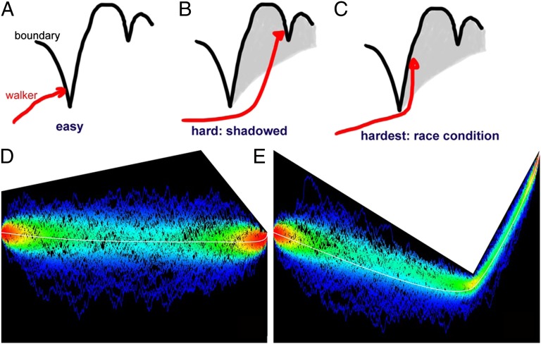
To develop some intuition about the problem, we are going to break it up into two parts, a “geometrical optics” part, in which most first passages can be accounted for by simple “visibility” considerations, and a “diffractive” correction in which we take into account that random walkers can turn around corners. The geometrical part is simple: most first passages are generated by the walker running into a hard-to-avoid obstacle, as shown in Fig. 1A. The intuition is that the walkers are moving left to right, rising onto a ceiling from which features are hanging, and as the walkers rise they collide with some feature. The problem is thus twice symmetry-broken: what matters are local minima of the boundary, not the maxima, which are hard to get into; and the walkers only spontaneously run onto the left flank of a local minimum. Therefore, a good first-order approximation follows from observing that most of the first passages occur on the left flanks of local minima, and deeper local minima cast “shadows” on subsequent shallower minima.

Fig. 1.

How a random walk V first hits a moving boundary L. In all panels, time t is horizontal, and the process V and the boundary L, vertical. (A) It is highly probable to hit the left flank of a minimum, as the walkers are moving left to right and from the bottom up. (B) Each minimum “casts a shadow” behind it, so that hitting some features behind may be hard, as it requires missing the minimum, then rising sufficiently high to hit the second feature. (C) Hitting the right (rising) flank of a minimum is hardest, because it requires missing the minimum narrowly, then rising up, setting up a “race condition” between the boundary and the walker. (D and E) Three hundred sample paths, which start at the red point on the left and have their first passage through the boundary (white) on the red point in the right. White curve: average trajectory (analytic). Sample paths are colored by the probability density of the point they go through. In D, hitting a left flank of a minimum is easy, and the average trajectory to do so does not significantly deviate from the deterministic trajectory until the very end, where the white curve can be seen to rise onto the minimum following a square root. In E, hitting the right flank of a minimum is hard, and the average trajectory to do so strongly deviates from the deterministic trajectories of the system, missing the minimum by just enough not to collide with it, and then rapidly rising to meet the first-passage point, again, in a square-root profile.

However, there is a finite probability that a walker may narrowly avoid a local minimum and pass just under it, only to rapidly rise afterward and hit the right rising flank of the barrier, as shown in Fig. 1C. This is, effectively, a race between the boundary and the walker: if the walker can rise far faster than the boundary, then there is some probability of passage right of the minimum. However, if the boundary rises faster than a walker can catch up with, then the probability of passage right of the minimum can be exponentially small. Let us consider a local minimum of the barrier B(t) at time t₀ of the following form:

and consider a walker that has just narrowly missed the minimum by an amount ε: W(t₀) = B(t) − ε. The probability of the process to be at value W at time t > t₀ is, to leading order,

where Γ is the diffusion constant of V_ξ, and thus the probability of arriving at the barrier at time t is approximately the following:

When H < 1/2, this expression has an essential singularity and has a value which is singular-exponentially small for small times. In fact, the probability and all of its derivatives are zero at t₀. For instance, consider a barrier whose flank to the right of the local minimum rises like . As the fourth root in the barrier rises much more rapidly than the square root in the walker, the probability of hitting the barrier after the minimum looks like , a function that has an essential singularity at 0: the function as well as all of its derivatives approach 0 as Δt → 0⁺.

The parameter H we described above, which is called the Hölder exponent of the function, quantifies the ability of the barrier to, locally, rise faster or slower than a random walk. More formally, a function f(t) is said to be H-Hölder continuous if it satisfies ; the roughness exponent H of the function is the largest possible value of H for which the function satisfies a Hölder condition.

Up to now, we have considered a single local minimum, and even though the probability of crossing is singular-exponential small for H < 1/2, it is still nonzero. However, if the boundary is rugged, the local minima are dense. This density is not an issue for H > 1/2, when the inputs are smoother than the internal noise; in this case the probability density of first passages is nowhere zero. However, when H < 1/2, the input is rougher or burstier than the internal noise; the probability density ceases to be a function, and it is zero almost everywhere except for a set of zero measure where it diverges.

Results

We shall present the more formal proofs of regularity of the first-passage time probability distributions elsewhere. We proceed now, instead, to present and analyze numerical simulations.

We carried out careful numerical integration of Eq. 1, with leak constant 10 ms, for all Hölder exponents H in the range (0.25–0.99) in increments of 0.01. In order for the results of the simulations at different Hölder exponents to be directly comparable with one another, we generated the inputs I(t) by using the exact same overall coefficients in the basis functions of the Ornstein–Uhlenbeck process described in ref. 61, but scaled differently according to the Hölder exponent laws in the natural way. For each one of the 75 Hölder exponents between 0.25 and 0.99, 62,000 repetitions of the 10-s stimulus were performed, accumulating 100,000,000 first passages per Hölder exponent. We computed the first passages using the fast algorithm described in refs. 56 and 61, which carries out exact integration in intervals which are recursively subdivided when the probability that the process attains the first passage exceeds a threshold, in our case 10⁻²⁰. The first passages were computed to an accuracy of 2⁻²⁶ = 1/67108864, and the allowable probability that a computed passage is not in fact the first one is p_fail = 10⁻¹⁵, so as to have an overall probability of 10⁻⁵ that any one of our 7.5 billion numbers is not in fact a true first passage. The values of the first passages were histogrammed in 22²² bins; this histogram, which we call our PSTH in analogy to the term in use in neural coding, represents the instantaneous probability distribution of first passage integrated over the bins, or, equivalently, the finite differences over a grid of the cumulative probability distribution function for firing.

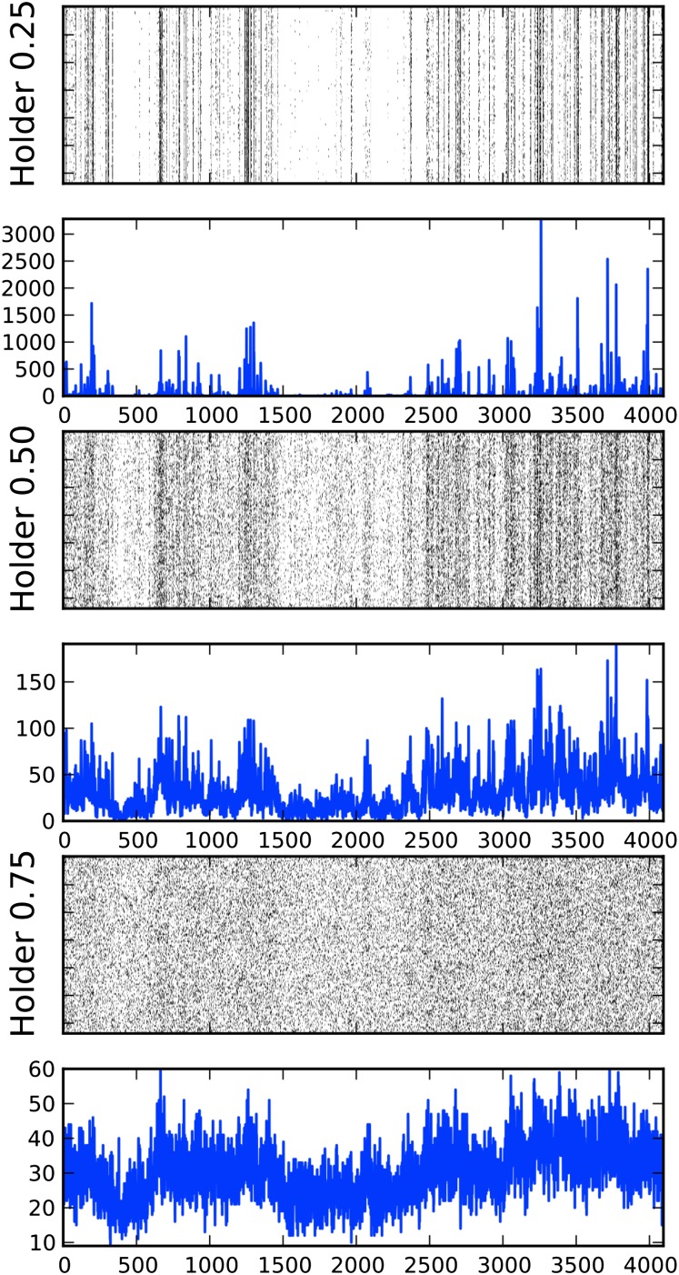
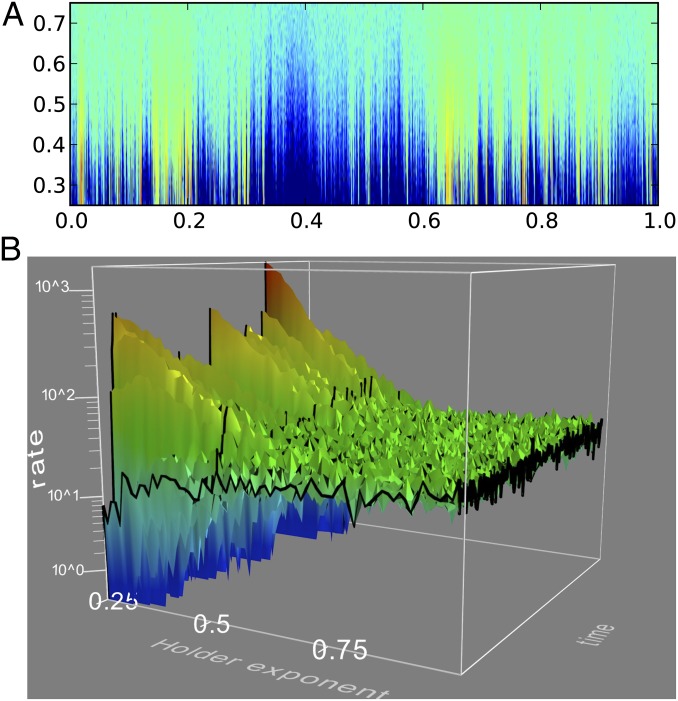
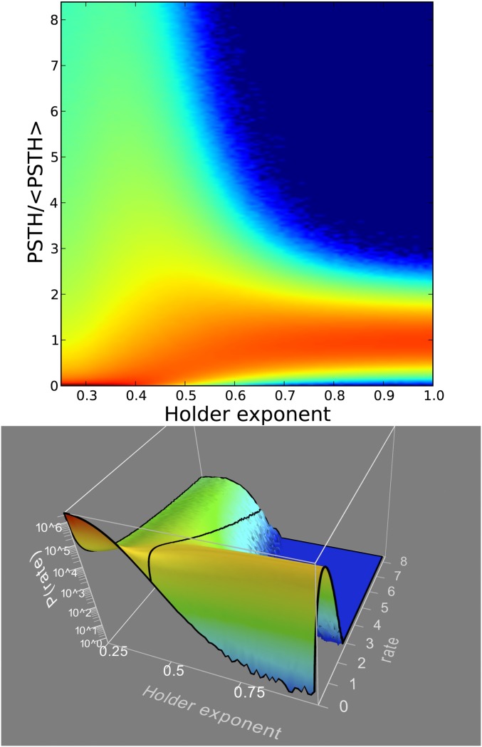
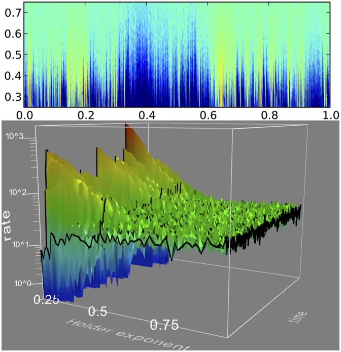
The transition from smooth probability distribution to a singular measure is illustrated in Figs. 2 and 3, where, as the Hölder exponent is lowered, the concentration of the first-passage probability on a small set is evident. Histogramming the individual bins of the PSTH, we get the probability distribution to observe a given instantaneous rate of firing, shown in Fig. 4. For large Hölder exponents, the rate does not deviate far from its mean. However, as the Hölder exponent becomes 1/2, both the probability of observing a zero rate, as well as the probability of seeing a rate far larger than the mean, become substantial. For H < 1/2, it becomes very probable to observe either zeros or large values of the instantaneous rate. This statement can be made precise by observing the tails of the probability distribution, and this is best accomplished, given our numerical setup, by looking at the tails of the cumulative probability distribution, namely the following:

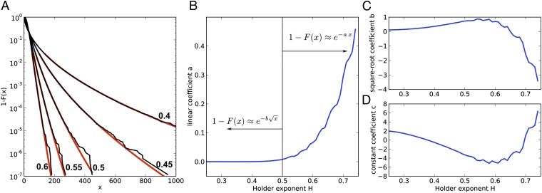
and then analyzing 1 − F(x) vs. x for large x, which is carried out in Fig. 5. Fig. 5A shows that the tails of the distribution, when x ≫ 1, decay exponentially for H > 1/2 but behave like stretched exponentials when H < 1/2 as follows:

This observation is quantified in Fig. 5B, where log(1 − F) is fitted with a quadratic polynomial in , namely the following:

For H < 1/2, the quadratic coefficient in the fit, which gives the convergent linear term, vanishes, uncovering the stretched exponential behavior. This quantitatively proves our assertion of a phase transition at H = 1/2.

Fig. 2.

Raster plots and PSTH. A small segment of our dataset, smaller than a leak constant, is displayed for clarity. A raster plot and a plot of the PSTH are shown for each of three Hölder exponents: 0.25 (rough), 0.5 (transition), and 0.75 (smoother, although still not differentiable). Approximately the same number of spikes occurs in all three groups. The raster plots display the times at which the neuron fired (i.e., a first passage) stacked vertically (as a function of stimulus presentation number) to show repeatability. The PSTHs show a temporal histogram of said spikes at extremely high resolution, a bin size in the microsecond range. Note the differences in vertical scale of the PSTHs: for Hölder exponent H = 0.75, there are no bins with fewer counts than 10 events or more than 60, whereas for H = 0.25 most bins have 0 counts and a few have over 1,000 counts.

Fig. 3.

(A) Probability density of firing as a function of time (horizontal) and Hölder exponent (vertical), color coded in log scale. Fifty-one values of the Hölder exponent H between 0.25 and 0.75 are stacked vertically. The bin counts shown in the PSTHs of Fig. 2 are color coded with a logarithmic code. (B) Three-dimensional rendering of a section of the data in A: vertical axis and color scale is logarithmic in the rate, where it is evident that toward the back of the figure (Hölder exponent H = 0.25) the rate either diverges or goes to zero almost everywhere.

Fig. 4.

Density map of PSTH bin counts. The individual bin counts of the PSTHs as shown in Figs. 2 and 3 are histogrammed here, and the value displayed as a logarithmic color map. All 7.5 billion spikes in our dataset were used for this plot. The bin counts are normalized by the average bin count (10⁸/2²²). For large Hölder exponents, the probability of observing an actual count agrees with counting statistics given the average. As the Hölder exponent becomes smaller, this distribution becomes wider, until below 0.5 it becomes heavy-tailed. Notice the bottom row of the figure, representing the probability of observing a bin with zero counts. It is zero for all H > 0.5, becomes nonzero at H = 0.5, and for H < 0.5 it is the maximum of the distribution (i.e., the brightest red value).

Fig. 5.

The tail of the cumulative probability distribution of observing a given count in the PSTH becomes a stretched exponential at Hölder exponent H = 0.5. (A) The tails of the cumulative probability distribution, plotted as 1 − F(x) vs. x, for Hölder exponents 0.4, 0.45, 0.5, 0.55, and 0.6 (right to left). The probability distribution is minus the derivative of these curves. Superposed on the data (black) a fit to the last 10⁵ data points in the cumulative, i.e., the higher 2% percentile (red), in the form . (B–D) The coefficients a, b, and c for the aforementioned fit, plotted as a function of the Hölder exponent H. B is a, the linear coefficient defining exponential convergence; C is b; and D is c. Notice that the linear component a is (numerically) zero for H < 0.5, exposing the term as the next higher order. For H > 0.5, the positive linear term guarantees convergence of all moments of the distribution.

Discussion

In abstract, mathematical terms, we have shown that the probability of observing a first passage of a Gauss–Markov process through a rough boundary of Hölder exponent H suffers a phase transition at H = 1/2. The integral of the probability on equispaced grids becomes a stretched exponential, showing the underlying instantaneous probability has ceased to be a function: it is concentrated on a Cantor-like set within which it is infinite, and it is zero outside this set. Gauss–Markov processes, such as the Ornstein–Uhlenbeck process, can be mapped to the canonical Wiener process through a deterministic joint scaling and time-change operation that preserves Hölder continuity. (This transformation is called Doob’s transform.) Furthermore, being the solution to a linear Langevin equation, the first-passage problem for drifted Gauss–Markov processes can always be formulated in terms of a fluctuating effective barrier that integrates the drift contribution. Therefore, our analysis directly applies to this situation. As nonlinear diffusions with bounded drift behave like Brownian motion at vanishingly small scales, we envision that our result is valid for this more general class of stochastic processes with Hölder continuous barrier. However, in this case, the barrier under consideration does not summarize the drift contribution of the diffusion.

In terms of the original motivating problem, the encoding of an input into the timing of action potentials by a model neuron, this means that within our (theoretical and rather aseptic) model, there is an abrupt transition in character of the PSTH, the instantaneous firing rate constructed from histogramming repetitions of the same stimulus. The transition happens when the input has the roughness of white noise, conceptually the case in which the neuron is receiving a barrage of statistically independent excitatory and inhibitory inputs, each with a random, Poisson character. For inputs that are smoother than this, the PSTH is a well-behaved function whose finite resolution approximations converge nicely and properly to finite values. However, when the input is rougher than uncorrelated excitation and inhibition, for example when excitatory and inhibitory activities are clustered positively with themselves and negatively with one another, then the PSTH is concentrated on a singularly small set, which means that the PSTH consists of a large number of sharply-defined peaks of many different amplitudes, but each one of them having precisely zero width. The width of the peaks is zero regardless of the amplitude of the internal noise; increasing internal noise only leads to power from the tall peaks being transferred to lower peaks, but all peaks stay zero width. Because the set of peaks is dense, refining the bins over which the PSTH is histogrammed leads to divergencies.

Concentration of the input into rougher temporal patterns would evidently be a function of the circuit organization. For example, in primary auditory cortex, the temporal precision observed in neuronal responses (62) appears to originate in the concentration of excitatory input into sharp “bump”-like features (63), an observation consistent with event-based analysis of spike trains (64). A network property that has been implicated in temporal precision is that of high-conductance states (65); it is plausible that, for carefully balanced recurrent excitation, leading to high gain states, such high-conductance states may lead to effectively bursty input to individual neurons.

It currently remains to be seen whether our mechanism will resist the multiple layers of real-world detail separating the abstract Eq. 1 from real neurons in a living brain. Obviously, the infinite sharpness of our mathematical result shall not withstand many relevant perturbations, which will broaden our zero-width peaks into finite thickness. That this will happen is indeed sure, but not necessarily relevant, because a defining characteristic of phase transitions is that their presence affects the parameter space around them even under strong perturbations: that is why studying phase transitions in abstract, schematic models has been fruitful. Thus, the real question remaining is whether our mechanism can retain enough temporal accuracy to be relevant to understand the organization of high–temporal-accuracy systems such as the auditory pathways, and whether our description of the roughness of the input as the primary determinant of coding modality, temporal code or rate code, may illuminate and inform further studies.

References

- 1.Risken H. The Fokker-Planck Equation: Methods of Solution and Applications. 2nd Ed. Berlin: Springer; 1996. [Google Scholar]
- 2.Wasan MT. 1994. Stochastic Processes and Their First Passage Times: Lecture Notes (Queen’s University, Kingston, ON, Canada)
- 3.Redner S. A Guide to First-Passage Processes. Cambridge, UK: Cambridge Univ Press; 2001. [Google Scholar]
- 4.van Kampen, NG 2007. Stochastic Processes in Physics and Chemistry (Elsevier, North-Holland Personal Library, Amsterdam)
- 5.Siegert AJF. On the 1st passage time probability problem. Phys Rev. 1951;81(4):617–623. [Google Scholar]
- 6.Mehr CB, Mcfadden JA. Explicit results for probability density of first-passage time for 2 classes of Gaussian-processes. Ann Math Stat. 1964;35(1):457–478. [Google Scholar]
- 7.Vanmarcke EH. Distribution of first-passage time for normal stationary random processes. J Appl Mech. 1975;42(1):215–220. [Google Scholar]
- 8.Domine M. Moments of the first-passage time of a Wiener process with drift between two elastic barriers. J Appl Probab. 1995;32(4):1007–1013. [Google Scholar]
- 9.Sacerdote L, Tomassetti F. On evaluations and asymptotic approximations of first-passage-time probabilities. Adv Appl Probab. 1996;28(1):270–284. [Google Scholar]
- 10.Kramers HA. Brownian motion in a field of force and the diffusion model of chemical reactions. Physica. 1940;7:284–304. [Google Scholar]
- 11.Strenzwilk DF. Mean first passage time for a unimolecular reaction in a solid. Bull Am Phys Soc. 1973;18(4):671. [Google Scholar]
- 12.Solc M. Time necessary for reaching chemical equilibrium: First passage time approach. Z Phys Chem. 2000;214:253–258. [Google Scholar]
- 13.Chelminiak P, Kurzynski M. Mean first-passage time in the steady-state kinetics of biochemical processes. J Mol Liq. 2000;86(1–3):319–325. [Google Scholar]
- 14.Arribas E, et al. Mean lifetime and first-passage time of the enzyme species involved in an enzyme reaction. Application to unstable enzyme systems. Bull Math Biol. 2008;70(5):1425–1449. doi: 10.1007/s11538-008-9307-4. [DOI] [PubMed] [Google Scholar]
- 15.Montroll EW. Random walks on lattices. 3. Calculation of first-passage times with application to exciton trapping on photosynthetic units. J Math Phys. 1969;10(4):753. [Google Scholar]
- 16.Ansari A. Mean first passage time solution of the Smoluchowski equation: Application to relaxation dynamics in myoglobin. J Chem Phys. 2000;112(5):2516–2522. [Google Scholar]
- 17.Goychuk I, Hänggi P. Ion channel gating: A first-passage time analysis of the Kramers type. Proc Natl Acad Sci USA. 2002;99(6):3552–3556. doi: 10.1073/pnas.052015699. [DOI] [PMC free article] [PubMed] [Google Scholar]
- 18.Kurzynski M, Chelminiak P. Mean first-passage time in the stochastic theory of biochemical processes. Application to actomyosin molecular motor. J Stat Phys. 2003;110(1–2):137–181. [Google Scholar]
- 19.Abdolvahab RH, Metzler R, Ejtehadi MR. First passage time distribution of chaperone driven polymer translocation through a nanopore: Homopolymer and heteropolymer cases. J Chem Phys. 2011;135(24):245102. doi: 10.1063/1.3669427. [DOI] [PubMed] [Google Scholar]
- 20.Roberts JB. Probability of first passage failure for stationary random vibration. AIAA J. 1974;12(12):1636–1643. [Google Scholar]
- 21.Kahle W, Lehmann A. 1998. Parameter estimation in damage processes: Dependent observation of damage increments and first passage time. Advances in Stochastic Models for Reliability, Quality and Safety (Birkhäuser, Boston), pp 139–152.
- 22.Khan RA, Ahmad S, Datta TK. 2003. First passage failure of cable stayed bridge under random ground motion. Applications of Statistics and Probability in Civil Engineering (IOS Press, Amsterdam), Vols. 1 and 2, pp 1659–1666.
- 23.Mazurek ME, Roitman JD, Ditterich J, Shadlen MN. A role for neural integrators in perceptual decision making. Cereb Cortex. 2003;13(11):1257–1269. doi: 10.1093/cercor/bhg097. [DOI] [PubMed] [Google Scholar]
- 24.Schmitt FG. Gamblers ruin problem. Am Math Mon. 1972;79(1):90. [Google Scholar]
- 25.Richter-Dyn N, Goel NS. On the extinction of a colonizing species. Theor Popul Biol. 1972;3(4):406–433. doi: 10.1016/0040-5809(72)90014-7. [DOI] [PubMed] [Google Scholar]
- 26.Saebø S, Almøy T, Heringstad B, Klemetsdal G, Aastveit AH. Genetic evaluation of mastitis resistance using a first-passage time model for Wiener processes for analysis of time to first treatment. J Dairy Sci. 2005;88(2):834–841. doi: 10.3168/jds.S0022-0302(05)72748-X. [DOI] [PubMed] [Google Scholar]
- 27.Lo CF. First passage time density for the disease progression of HIV infected patients. Lect Notes Eng Comp. 2006;62:117–122. [Google Scholar]
- 28.Xu RM, McNicholas PD, Desmond AF, Darlington GA. A first passage time model for long-term survivors with competing risks. Int J Biostat. 2011;7(1):1224–1227. [Google Scholar]
- 29.Ammann M. Credit Risk Valuation: Methods, Models, and Applications. 2nd Ed. New York: Springer; 2001. [Google Scholar]
- 30.Zhang D, Melnik RVN. First passage time for multivariate jump-diffusion processes in finance and other areas of applications. Appl Stoch Model Bus. 2009;25(5):565–582. [Google Scholar]
- 31.Yi CA. On the first passage time distribution of an Ornstein-Uhlenbeck process. Quant Finance. 2010;10(9):957–960. [Google Scholar]
- 32.Capocelli RM, Ricciardi LM. Diffusion approximation and first passage time problem for a model neuron. Kybernetik. 1971;8(6):214–223. doi: 10.1007/BF00288750. [DOI] [PubMed] [Google Scholar]
- 33.Mainen ZF, Sejnowski TJ. Reliability of spike timing in neocortical neurons. Science. 1995;268(5216):1503–1506. doi: 10.1126/science.7770778. [DOI] [PubMed] [Google Scholar]
- 34.Shimokawa T, Pakdaman K, Takahata T, Tanabe S, Sato S. A first-passage-time analysis of the periodically forced noisy leaky integrate-and-fire model. Biol Cybern. 2000;83(4):327–340. doi: 10.1007/s004220000156. [DOI] [PubMed] [Google Scholar]
- 35.Agüera y Arcas B, Fairhall AL, Bialek W. Computation in a single neuron: Hodgkin and Huxley revisited. Neural Comput. 2003;15(8):1715–1749. doi: 10.1162/08997660360675017. [DOI] [PubMed] [Google Scholar]
- 36.Agüera y Arcas B, Fairhall AL. What causes a neuron to spike? Neural Comput. 2003;15(8):1789–1807. doi: 10.1162/08997660360675044. [DOI] [PubMed] [Google Scholar]
- 37.Sacerdote L, Zucca C. 2005. Inverse first passage time method in the analysis of neuronal interspike intervals of neurons characterized by time varying dynamics. Brain, Vision, and Artificial Intelligence: Proceedings of the First International Symposium, BVAI 2005, Naples, Italy, October 19–21, 2005, (Springer, Berlin), Vol. 3704, pp. 69–77.
- 38.Fauchald P, Tveraa T. Using first-passage time in the analysis of area-restricted search and habitat selection. Ecology. 2003;84(2):282–288. [Google Scholar]
- 39.Le Corre M, et al. A multi-patch use of the habitat: Testing the first-passage time analysis on roe deer Capreolus capreolus paths. Wildl Biol. 2008;14(3):339–349. [Google Scholar]
- 40.Noh JD, Rieger H. Random walks on complex networks. Phys Rev Lett. 2004;92(11):118701. doi: 10.1103/PhysRevLett.92.118701. [DOI] [PubMed] [Google Scholar]
- 41.Condamin S, Bénichou O, Tejedor V, Voituriez R, Klafter J. First-passage times in complex scale-invariant media. Nature. 2007;450(7166):77–80. doi: 10.1038/nature06201. [DOI] [PubMed] [Google Scholar]
- 42.Buonocore A, Nobile AG, Ricciardi LM. A new integral-equation for the evaluation of 1st-passage-time probability densities. Adv Appl Probab. 1987;19(4):784–800. [Google Scholar]
- 43.Lo CF, Hui CH. Computing the first passage time density of a time-dependent Ornstein-Uhlenbeck process to a moving boundary. Appl Math Lett. 2006;19(12):1399–1405. [Google Scholar]
- 44.Peskir G, Shiryaev AN. On the Brownian first-passage time over a one-sided stochastic boundary. Theory Probab Appl. 1998;42(3):444–453. [Google Scholar]
- 45.Rieke F. Spikes: Exploring the Neural Code. Cambridge, MA: MIT; 1997. [Google Scholar]
- 46.Abbott LF, Sejnowski TJ. Neural Codes and Distributed Representations: Foundations of Neural Computation. Cambridge, MA: MIT; 1999. [Google Scholar]
- 47.Tiesinga P, Fellous JM, Sejnowski TJ. Regulation of spike timing in visual cortical circuits. Nat Rev Neurosci. 2008;9(2):97–107. doi: 10.1038/nrn2315. [DOI] [PMC free article] [PubMed] [Google Scholar]
- 48.Cecchi GA, et al. Noise in neurons is message dependent. Proc Natl Acad Sci USA. 2000;97(10):5557–5561. doi: 10.1073/pnas.100113597. [DOI] [PMC free article] [PubMed] [Google Scholar]
- 49.Arcas BAY, Fairhall AL, Bialek W. What can a single neuron compute? Adv Neur In. 2001;13:75–81. [Google Scholar]
- 50.Tiesinga PHE, Sejnowski TJ. Precision of pulse-coupled networks of integrate-and-fire neurons. Network. 2001;12(2):215–233. [PubMed] [Google Scholar]
- 51.Beierholm U, Nielsen CD, Ryge J, Alstrøm P, Kiehn O. Characterization of reliability of spike timing in spinal interneurons during oscillating inputs. J Neurophysiol. 2001;86(4):1858–1868. doi: 10.1152/jn.2001.86.4.1858. [DOI] [PubMed] [Google Scholar]
- 52.Tiesinga PHE, Fellous JM, Sejnowski TJ. Spike-time reliability of periodically driven integrate-and-fire neurons. Neurocomputing. 2002;44:195–200. [Google Scholar]
- 53.Brette R, Guigon E. Reliability of spike timing is a general property of spiking model neurons. Neural Comput. 2003;15(2):279–308. doi: 10.1162/089976603762552924. [DOI] [PubMed] [Google Scholar]
- 54.Lo CF, Chung TK. 2006. First passage time problem for the Ornstein-Uhlenbeck neuronal model. Neural Information Processing (Springer, Berlin), Vol. 4232, pp. 324–331.
- 55.Buonocore A, Caputo L, Pirozzi E, Ricciardi LM. 2009. On a generalized leaky integrate-and-fire model for single neuron activity. Computer Aided Systems Theory—Eurocast 2009 (Springer, Berlin), Vol. 5717, pp 152–158.
- 56.Taillefumier T, Magnasco MO. A fast algorithm for the first-passage times of Gauss-Markov processes with Hölder continuous boundaries. J Stat Phys. 2010;140(6):1130–1156. [Google Scholar]
- 57.Buonocore A, Caputo L, Pirozzi E, Ricciardi LM. On a stochastic leaky integrate-and-fire neuronal model. Neural Comput. 2010;22(10):2558–2585. doi: 10.1162/NECO_a_00023. [DOI] [PubMed] [Google Scholar]
- 58.Buonocore A, Caputo L, Pirozzi E, Ricciardi LM. The first passage time problem for Gauss-diffusion processes: Algorithmic approaches and applications to LIF neuronal model. Methodol Comput Appl. 2011;13(1):29–57. [Google Scholar]
- 59.Dong Y, Mihalas S, Niebur E. Improved integral equation solution for the first passage time of leaky integrate-and-fire neurons. Neural Comput. 2011;23(2):421–434. doi: 10.1162/NECO_a_00078. [DOI] [PMC free article] [PubMed] [Google Scholar]
- 60.Thomas PJ. A lower bound for the first passage time density of the suprathreshold Ornstein-Uhlenbeck process. J Appl Probab. 2011;48(2):420–434. [Google Scholar]
- 61.Taillefumier T, Magnasco MO. A Haar-like construction for the Ornstein Uhlenbeck process. J Stat Phys. 2008;132(2):397–415. [Google Scholar]
- 62.Elhilali M, Fritz JB, Klein DJ, Simon JZ, Shamma SA. Dynamics of precise spike timing in primary auditory cortex. J Neurosci. 2004;24(5):1159–1172. doi: 10.1523/JNEUROSCI.3825-03.2004. [DOI] [PMC free article] [PubMed] [Google Scholar]
- 63.DeWeese MR, Zador AM. Non-Gaussian membrane potential dynamics imply sparse, synchronous activity in auditory cortex. J Neurosci. 2006;26(47):12206–12218. doi: 10.1523/JNEUROSCI.2813-06.2006. [DOI] [PMC free article] [PubMed] [Google Scholar]
- 64.Toups JV, et al. Finding the event structure of neuronal spike trains. Neural Comput. 2011;23:1–40. doi: 10.1162/NECO_a_00173. [DOI] [PMC free article] [PubMed] [Google Scholar]
- 65.Destexhe A, Rudolph M, Paré D. The high-conductance state of neocortical neurons in vivo. Nat Rev Neurosci. 2003;4(9):739–751. doi: 10.1038/nrn1198. [DOI] [PubMed] [Google Scholar]