Large scale chromosomal mapping of human microRNA structural clusters

Abstract

MicroRNAs (miRNAs) can group together along the human genome to form stable secondary structures made of several hairpins hosting miRNAs in their stems. The few known examples of such structures are all involved in cancer development. A large scale computational analysis of human chromosomes crossing sequence analysis and deep sequencing data revealed the presence of >400 structural clusters of miRNAs in the human genome. An a posteriori analysis validates predictions as bona fide miRNAs. A functional analysis of structural clusters position along the chromosomes co-localizes them with genes involved in several key cellular processes like immune systems, sensory systems, signal transduction and development. Immune systems diseases, infectious diseases and neurodegenerative diseases are characterized by genes that are especially well organized around structural clusters of miRNAs. Target genes functional analysis strongly supports a regulatory role of most predicted miRNAs and, notably, a strong involvement of predicted miRNAs in the regulation of cancer pathways. This analysis provides new fundamental insights on the genomic organization of miRNAs in human chromosomes.

INTRODUCTION

MicroRNAs (miRNAs) are small 18–25-nt regulatory RNAs modulating gene expression in animals and plants. The number of discovered miRNAs has increased from tens to thousands and is likely to grow further. Most miRNAs discovered first were found to be highly conserved, and many of those discovered more recently appear to be shared by a smaller number of phylogenetically close species. In some cases, they belong to a single species, and it is hypothesized that they establish and maintain phenotypic diversity between different groups of organisms (1). The miRNAs play an important role in diverse physiological and developmental processes by negatively regulating expression of target genes at the post-transcriptional level. Current estimates suggest that the human genome contains at least hundreds of distinct miRNAs that regulate a large fraction of the transcriptome (2–6).

The proportion of human miRNAs organized in clusters, i.e. chromosomal regions of variable length reaching sizes as 50 kb and containing several miRNAs (7), is significantly higher than expected (2,4). Genomic organization of 326 human miRNAs (in miRNA registry 7.1) has been analysed in (8) where 148 human miRNAs were identified to be localized in 51 clusters. Within intergenic regions, these clusters were defined by considering miRNAs at a distance smaller than 3000 nt. Within an intron, clusters are formed by considering all miRNAs that are contained in it, without asking for any distance constraint. Alignment of miRNA sequences lying within the same cluster or in different clusters revealed a significant number of miRNA paralogs shared among and within clusters, implying an evolution process targeting the potentially conserved roles of these molecules.

A miRNA structural cluster is a cluster of miRNAs, which is situated in a region typically smaller than 1–2 kb and which folds into a secondary structure presenting several hairpins, where miRNAs are located within the stems. Such structures may contain several paralogous miRNAs. Structural clusters of miRNAs are stable structures that are supposed to form in the cell to avoid immediate degradation. The idea being that the region may be transcribed into a single non-coding RNA precursor, which is then processed to give rise to several individual miRNA precursors possibly collaborating for a common functional purpose. The known miRNA clusters mir-17-92 (9) and mir-106a-363 (10) satisfy such structural conditions, and we looked for others having the same characteristics in the human genome (see Figure 1). Notice that miRNA clusters mir-17-92 and mir-106a-363 are known to play a role in human tumour development (9–11) and that the identification of other potential structural clusters involved in human diseases is of clear importance in genetics and medicine. The computational challenge is not obvious; one needs not just to search for regions localizing potential miRNAs similar to known ones but rather search for regions forming a stable secondary structure with hairpin characteristics described earlier in the text.

Figure 1.

Four examples of structural clusters predicted by the algorithm. (a): structural cluster, known as mir-17-92, predicted on human chromosome 13 from deep-sequencing data. (b): structural cluster, known as mir-106a-363, predicted on human chromosome X from deep-sequencing data. (c): Structural cluster predicted on human chromosome 19 from paralogous sequences. (d): Structural cluster predicted on human chromosome 22 by combining paralogous sequences and deep-sequencing data. In (a) and (b), miRNAs validated by the algorithm are highlighted in blue. In (c) and (d), miRNAs validated by the algorithm are highlighted in red (similar sequences) or blue (deep-sequencing reads). All structural clusters were filtered with RepeatMasker.

We propose a novel and original algorithm to discover structural clusters of miRNAs. Contrary to the method developed in (12), we do not start from regions surrounding already known miRNAs but rather search for those regions along the genome, which are rich of palindromic sequences, these regions being good candidates for localizing structural clusters containing several paralogs. Our strategy makes the approach ab initio, as no a priori knowledge on miRNAs is used to reduce search space. No comparative genomics is used either. The method has been adapted to infer structural clusters directly from the mapping of deep-sequencing reads on the genome (bypassing palindromic search). Along with structural clusters, the algorithm identifies novel potential miRNAs and their corresponding precursors (pre-miRNAs). The pre-miRNAs have been selected using MIReNA (13), a tool that has already been proven to successfully predict pre-miRNAs in plant (14) and was declared a first-choice when predicting new miRNAs in mammals (15). An a posteriori analysis, based on a series of expected characteristics of miRNAs and pre-miRNAs, validates our predictions as bona fide miRNAs.

Based on our predictions of structural clusters, we propose a genetic identification of chromosomal regions that are susceptible to contain important information on regulation of several key cellular processes by predicted miRNA genes. We identify prime candidates for miRNA-mediated regulation within several functional classes of genes but also within groups of genes involved in human diseases. The miRNA target analysis confirms a regulatory role of most predicted miRNAs in structural clusters.

MATERIALS AND METHODS

Algorithm

Structural clusters of miRNAs are identified along a genome either by an ab initio sequence analysis or by a structural analysis based on deep-sequencing data or by a combination of the two. The algorithm starts with a pre-treatment of the genomic sequence and filters afterwards potential miRNA structural clusters based on five combinatorial and structural criteria describing acceptable pre-miRNAs (13). Then, it predicts structural clusters either by looking for repeated sequences in palindromic regions (black path, Figure 2), by using deep-sequencing reads as potential miRNAs forming structural clusters (red path, Figure 2) or by combining the two kinds of information, i.e. by finding structural clusters from deep-sequencing reads and from multiple palindromic sequences (green path, Figure 2).

Figure 2.

MIReStruC: an algorithm searching for miRNA structural clusters along a genome. The search starts either from repeated (similar) sequences in palindromic regions (black path) or from deep-sequencing data (red path). Predictions can also be made by combining the two kinds of information (green path).

Ab initio search based on sequence analysis

Given a genome, the algorithm looks for regions containing palindromic sequences and identifies those regions in the genome containing several palindromes. It makes no use of an a priori bound on the size of these regions (once applied to the human genome, the algorithm analysed palindromic regions of a minimum size of 426 nt and a maximum size of 35 080 nt in length, with an average of 933 nt and a standard deviation of 416 nt of the distribution of sizes). Then, it extracts sequences of ∼22 nt that are repeated (by allowing for some possible errors in repetitions) within palindromic regions. These sequences are considered as potential paralogous miRNA sequences, and we ask them to be at least three within the region. The threshold comes from the characteristics of known clusters, mir-17–92 and mir-106a-363 considered in (16,17). From predicted putative miRNA sequences, corresponding putative pre-miRNAs, if any, are predicted [by using five structural and combinatorial criteria (13)]. The full structure of the clusters of miRNAs is validated to satisfy some extra structural conditions.

In the following, we call miRNA* the complementary sequence (possibly including unpaired nucleotides) of the miRNA r within a pre-miRNA structure. Given a pre-miRNA sequence s, the Adjusted Minimum Folding Energy (AMFE)(s) (18) is computed as , where MFE(s) stands for the minimum free energy of s (19,20) (and measures the stability of the secondary structure by taking into account empirical energy parameters associated to base pairs, base pairs stacks, bulge and hairpin loops and various motifs, which are known to occur with great frequency) and l(s) is the length, i.e. the number of nucleotides, of s. The Minimum Free Energy Index MFEI(s) (18) is computed as , where % stands for the percentage of G + C composition of s. The steps of the algorithm (black path, Figure 2) are as follows:

1. Palindromic sequences and clusters of palindromes are identified and filtered in such a way that only those that contain at least three paralogous sequences of ∼22 nt in length are retained (see later in the text for details). Such paralogous sequences will be treated as potential miRNAs (on either strands).

2. Potential miRNAs are extended on the left and on the right by 200 nt on each side.

3. Using MiReNA (13), we compute secondary structures of all extended sequences containing the potential miRNA and scanned them to filter out those that do not satisfy suitable combinatorial and physico-chemical conditions. The resulting structures are considered as putative pre-miRNAs. For all potential miRNAs contained in them, we treat overlapping ones with MiReNA and select those miRNAs with most stable matching or, in case of equal stability of the matching (i.e. equal MFE value), longest sequence.

4. The remaining potential miRNAs are grouped together in clusters satisfying suitable proximity conditions: (i) two miRNAs belong to the same cluster if their distance is smaller than 300 nt and (ii) a cluster should contain at least three miRNAs. Once a group of miRNAs is identified to be locally close, we define the cluster to be the minimal sequence containing the associated pre-miRNAs.

5. For each cluster of miRNAs, we slide a window of ∼1000 nt along the cluster (as described later in the text) and for each window:

   1. We compute the secondary structure using RNAfold (21)
   2. We tag as ‘valid’ those miRNAs that best match stems, i.e. satisfying the validation criteria described later in the text.

6. We apply again step 4 by only considering miRNAs that are flagged ‘valid’ in at least one window. This might lead to the detection of new clusters.

7. Steps 4 and 5 are re-iterated until the set of valid miRNAs remains unchanged.

8. For each resulting cluster sequence, we perform a and b in step 5. The associated structure may be larger than those obtained by looking at windows, and the validity of miRNAs is tested again.

9. Given a cluster, we filter miRNAs by only keeping those that have at least two paralogous miRNAs within the cluster. Paralogous miRNAs are grouped together to form new clusters, and they are analysed as in step 7. The resulting clusters are structural clusters.

10. (Optional) structural clusters of miRNAs are filtered to keep those that contain Expressed Sequence Tags (EST) [by using BLAST in dbEST (22)] or to remove those containing repeats [by using RepeatMasker, version: open-3.2.8 (RMlib: 20090604), A. Smit, R. Hubley and P. Green, unpublished data, 2009)]. Note that a structural cluster rejected by RepeatMasker might be kept when EST data support its existence, and that a structural cluster passing the RepeatMasker filter does not need to match EST data to be retained.

11. (Optional) structural clusters of miRNAs are filtered to remove those overlapping Coding Sequences (CDS), exons and non coding RNAs (ncRNA) (on either strands).

The algorithm provides a list of positions of structural clusters of paralogous miRNAs together with the positions of their miRNAs and the associated pre-miRNAs.

To illustrate the complexity of the ab initio structural clusters search, it is useful to consider the number of intermediate structures analysed at different steps: in step 1, the number of clusters of palindromes is , and the number of potential miRNAs tested on either strands is ; in step 3, the number of potential miRNAs after pre-miRNAs prediction is ; in step 4, the number of potential miRNAs after clusterization is , and the number of corresponding clusters is ; at the end of the algorithm, after cluster’s structural validation (steps 5 and 6) and after filtering with RepeatMasker and EST data (step 9) and with CDS/exons/ncRNA locations (step 10), the number of potential miRNAs is 1334, and the number of potential structural clusters is 300. Notice that after step 9, only ∼10% of predictions overlap CDS/exons/ncRNAs. Namely, the number of structural clusters obtained after applying RepeatMasker before CDS/exons/ncRNAs filtering is 199 and after CDS/exons/ncRNAs filtering is 182; for EST data, it is 182 and 160.

The different steps of the algorithm are treated in detail in the following.

Search of clusters of palindromes

A palindromic sequence s is composed of two complementary subsequences s₁ and s₂ and of the sequence s_e lying between s₁ and s₂. The s may potentially form an hairpin secondary structure. We do not ask for a perfect complementarity between s₁ and s₂ within the structure, but we define a complementarity score ps (for ‘palindromic score’) for evaluating a match. The complementarity score of a palindrome is computed on the match between s₁ and s₂ as the sum of weights given to Watson–Crick/Wobble complementary nucleotide pairs and of penalties given to gap opening and gap extension (see later in the text for a rigorous definition). Acceptable palindromes are characterized by several parameters: minimal and maximal lengths of the palindrome, minimal and maximal lengths of s_e, the complementarity score and a relativized complementarity score ps_rel. Suitable thresholds for these parameters have been calculated by studying the distribution of values of the parameter on all human pre-miRNAs in miRBase v14 (23–25) and by considering as a threshold (respectively if minimal values are bounded), where μ and σ are mean and standard deviation of the distribution.

Searching for palindromic sequences

Given a sequence, a dynamic programming algorithm searches for a hairpin structure within the sequence and for the two subsequences s₁ and s₂ in the hairpin sequence s forming the hairpin stem that best maximizes the complementarity score ps and best minimizes the length of the loop s_e. The complementarity score is computed between s₁ and s₂, and it is used to filter pairs of palindromic sequences along a genome. Strictly speaking, the algorithm slides a window (whose length corresponds to the maximal length of an accepted palindromic sequence) along the genomic sequence and constructs a matrix (representing all possible matching) by locally maximizing the complementarity score for the nucleotide positions , following Gotoh’s algorithm (26), where weight 1 is given to Watson–Crick pairing, 0.8 to Wobble, −1 to gap opening and −0.2 to gap extension. The reconstruction of the best matching is done by backtracking on the matrix construction starting from its maximum value at . The score is the complementarity score associated to s, where n₀ is the position of the first paired nucleotide of s, and m₀ is the position of the last paired nucleotide of s. The n₀-th and m₀-th positions are paired together. The relativized complementary score is defined as .

Identification of clusters of palindromes

Positions of palindromic sequences known, we look for regions that contain clusters of palindromes. By transitivity, we define groups of overlapping palindromes along the genomic sequence. For each group, we estimate the number of non-overlapping palindromes by dividing the number of covered nucleotides by the minimal length of a palindrome (set at 71 nt by default). Then, groups of palindromes (possibly overlapping) are gathered together (by transitivity) in clusters if their distances is at most 120 nt. The number of non-overlapping palindromes in such clusters is the sum of non-overlapping palindromes estimated in each group. We ask for a cluster to contain at least six non-overlapping palindromes to be further considered in our analysis.

Treatment of paralogous sequences in clusters of palindromes

To search for repeated sequences of ∼22 nt in length within clusters of palindromes, step 1 of the algorithm (black path, Figure 2) uses an adapted version of the approximate string matching algorithm described in (27). It applies it within a sliding window of 500 nt running along clusters of palindromes. For each window, step 1 considers the first 22 nt of the window and looks for similar sequences within the window, i.e. for a sequence of at most 25 nt in length and displaying at most 19% of differences (corresponding to nucleotide insertion, substitution and deletion) from the initial sequence (28). Paralogous sequences that occur at least three times within a window are considered as potential miRNAs.

Validation of miRNAs in structural clusters

The miRNAs in a cluster are validated by looking at their associated pre-miRNA structures. A window of 1000 nt is slided over the cluster sequence and positioned at the start of each pre-miRNA associated to some putative miRNA in the cluster until all miRNAs have been considered by at least one window. For each window, we extract the minimal subsequence that contains all pre-miRNAs lying within the window. The secondary structure corresponding to the entire subsequence is computed with RNAfold. A miRNA r is tagged as ‘valid’ if the following conditions hold:

1. It completely lies in a stem.

2. It satisfies the inequalities and where P(r) corresponds to the percentage of unmatched nucleotides of r.

3. It is the best match on its stem, i.e. for any other potential miRNA r₂ within the stem, the free energy associated to r (together with its complement ) is lower than the one of r₂ (with ). The MFE is computed with RNAeval (21).

Thresholds in condition 2 are less strict than the ones used to validate pre-miRNA structures in (13). This choice is due to the fact that, here, we consider the structure of several pre-miRNAs all together instead of just one. The thresholds are computed as in (13) by looking at the distribution of distances between r and (defined as for miRNAs in the miRBase data set and by using at least as an acceptable distance, where μ and σ are mean and standard deviation of the distribution). The threshold on the percentage of unmatched nucleotides is computed as , where and are mean and standard deviation of the distribution of values computed on the miRBase v14 data set. These thresholds validate the miRNAs occurring in the two known structural clusters mir-17–92 and mir-106a-363.

A miRNA is ‘valid’ for the cluster if it is ‘valid’ in at least one window.

No reasonable prediction system assessment (evaluating sensitivity, specificity and accuracy of the method) can be performed, as too few structural clusters are known. Examples are mir-17-92 and mir-106a-363, both detected by our methods based on paralogous sequences and on deep-sequencing data. It should be reminded that it is the very limited knowledge of structural clusters that motivated this study. The validation of miRNAs lying in structural clusters has been extensively tested though. Predictions were performed using the MIReNA algorithm (13). MIReNA has been extensively compared with other systems by computing sensitivity, specificity, accuracy and Matthew correlation coefficient (13). An independent study (15) declared MIReNA to be the first choice over nine tools devoted to the prediction of new miRNAs in mammalian genomes. Also, MIReNA was used to successfully predict a large and robust data set of miRNA homologues that complemented and refined the reference miRBase catalogue leading to novel discoveries on conservation patterns between monocot and eudicot genomes (14).

Search based on deep-sequencing data

The algorithm is designed to search for miRNA structural clusters from deep-sequencing data (red path, Figure 2). Deep-sequencing reads are mapped on the genome using MicroRazerS (29), and each of them is considered as a potential miRNA sequence. The algorithm goes essentially as the one described earlier in the text: it starts from step 2 and skips step 10, as no paralogy is tested on deep-sequencing reads. It outputs potential miRNAs grouped in structural clusters where each miRNA corresponds to a read.

Search based on the combination of deep-sequencing data and paralogous sequences

The algorithm combines deep-sequencing reads and paralogous sequences within clusters of palindromes (green path, Figure 2). Step 1 considers two similar sequences (instead of a minimum of three, as for the black path) in genomic regions with several palindromes and including deep-sequencing reads. Paralogous sequences and deep-sequencing reads are considered as potential miRNAs and grouped together into clusters. Step 10 of the algorithm validates structural clusters with at least one deep-sequencing read and two paralogous sequences.

Comparison of structural clusters identified by different methods

Two structural clusters, predicted by different methods, are considered to be the same if their corresponding sequences overlap. No condition on the size of the overlapping is imposed.

The miRNA targets predictions

Predictions of miRNA targets are realized with miRanda (30,31) starting from 33 810 3′ untranslated region (UTR) and 326 741 CDS sequences obtained at the UCSC site (http://genome.ucsc.edu, tables, hg18, RefSeq genes, 3′UTR, exons). The same gene can be associated to several 3′UTRs in case of multiple transcripts. Target analysis was done for the 1713 potential miRNAs in structural clusters. The miRanda was run with default parameters: score and miRNA/target energy . It predicted 14 450 583 miRNA/3′UTR pairs. To discriminate the huge number of miRNA/3′UTR pairs, we considered mean and standard deviation of the associated energy distribution and analysed in detail the sets of predicted pairs with energy , where c can be either 2 or 3. This means 394 005 and 50 805 miRNA/3′UTR pairs, respectively. The first set involves 1263 (73.73%) miRNAs (located in 349 different structural clusters) and 20 264 3′UTRs, and the second set involves 623 (36.72%) miRNAs (located in 229 different clusters) and 9316 3′UTRs.

The miRanda predicted 16 028 721 miRNA/CDS pairs. As for 3′UTR regions, to discriminate the huge number of miRNA/CDS pairs, we considered mean and standard deviation of the associated energy distribution and analysed in detail the sets of predicted pairs with energy , where c can be either 2 or 3. This means 458 697 and 50 057 miRNA/CDS pairs, respectively. The first set involves 1239 (72.33%) miRNAs (located in 342 different structural clusters) and 79 271 CDSs, and the second involves 589 (34.38%) miRNAs (located in 213 different clusters) and 18 846 3′UTRs.

Then, 3′UTR and CDS were further analysed to predict miRNA targets with the Probability of Interaction by Target Accessibility (PITA) algorithm (32) based on hybridization energy and site accessibility (Supplementary Data Set 5).

Functional analysis of targets

To realize a functional analysis of the potential targets of our predicted miRNAs, we used the Database for Annotation, Visualization and Integrated Discovery (DAVID) v6.7 (33,34). Given a set of RefSeq mRNAs containing potential targets, DAVID extracted, whenever possible, those gene ontology (GO) terms classified as biological processes (BP) and molecular functions (MF), Kyoto Encyclopedia of Genes and Genomes (KEGG) pathways or Protein Information Resource (PIR) keywords that were over-represented in the set of genes. The results of the analysis are reported in the folders in Supplementary Data Set 4, where one finds a list of enriched functions, the associated P-value (DAVID EASE score), the fold enrichment value and the Benjamini-corrected P-value obtained after multiple testing corrections.

Filters for structural clusters

Structural cluster predictions were filtered by using Homo sapiens EST data from dbEST (22). The match was done with BLAST at http://blast.ncbi.nlm.nih.gov run with default parameters. Only structural clusters aligning an EST with an were retained.

RepeatMasker has been used as a filter to remove sequences containing repeats. We used version open-3.2.8 with RMLib:20090604 at http://www.repeatmasker.org/cgi-bin/WEBRepeatMasker and cross-match as search engine with a slow speed. Repeat sequences used by RepeatMasker are stored in Repbase (35).

Human genome and fragile sites

Human genome (BUILD 36.3) flat files have been retrieved from NCBI website (www.ncbi.nlm.nih.gov). Positions of chromosomal bands were obtained at ftp://ftp.ncbi.nih.gov/genomes/MapView/Homo_sapiens sequence/BUILD36.3/initial_release/ideogram.gz. The list of fragile sites comes from (36), where each fragile site is associated to a chromosomal band. Positions of chromosomal bands were used to obtain positions of fragile sites.

Data sets

Known miRNA sequences were retrieved from miRBase v.16 at www.mirbase.org (collecting miRNAs from 142 species), and we used them for making the analysis based on paralogous sequences. The miRBase v.13 (corresponding to the human genome assembly that we analysed) was used to determine the coverage of miRNAs lying in fragile sites and structural cluster regions (23–25).

Several sets of deep-sequencing reads were used to predict structural clusters. Data sets were retrieved from the Gene Expression Omnibus database at NCBI (http://www.ncbi.nlm.nih.gov/geo/) and from the Sequence Read Archive at NCBI (http://www.ncbi.nlm.nih.gov/sra/ (see Supplementary Table S1 for accession numbers). Among deep-sequencing data coming from the Sequence Read Archive, some were extracted from breast cancer cells (SRR015446, SRR015447 and SRR015448), and the others from 12 melanoma and pigment cells. Reads coming from Gene Expression Omnibus archive, originate from cell lines derived from cervical cancer cells (GSE14362 and GSE10829), small RNAs from human embryonic stem cells, derived neural progenitors and neurons (GSE13483), endogenous small RNAs associated to human Argonaute 1 and 2 (GSE13370). Predictions are made by putting together reads from all experiments, but the origin of the deep-sequencing read appearing in a predicted structural cluster is indicated in Supplementary Data Set 2.

Sets of deep-sequencing reads were mapped to the human genome and filtered with MicroRazerS (29) that imposes that the same sequence cannot match more than five different positions in the genome.

Three data sets of genes involved in different biological pathways have been used:

1. KEGG PATHWAY database: it is a collection of manually drawn pathway maps representing the knowledge on the molecular interaction and reaction networks for metabolism, genetic information processing, environmental information processing, cellular processes, organismal systems and human diseases (37,38). The 209 biological pathways defined for H. sapiens are organized in a hierarchy of classes and subclasses that we used in our analysis (Supplementary Table S2). Data have been retrieved at www.genome.jp/kegg/pathway.html.

2. Atlas of Genetics and Cytogenetics in Oncology and Haematology (ATLAS): it is a collection of genes associated to cancer (39–45). Data were retrieved from http://atlasgeneticsoncology.org/Genes/Gene liste.html (indexation of May 28, 2010).

3. Cancer Gene Census (CGC): a data set of genes known to undergo mutations in cancer (46). Data have been retrieved from www.sanger.ac.uk/genetics/CGP/Census/Table_1_full_2010_03_30.xls.

Structural cluster regions

To analyse structural clusters localization on human chromosomes, we defined structural cluster regions. Given a distance δ, we say that two structural clusters occur in the same structural cluster region if their distance (computed by considering the two closer extremes) is at most δ. By transitivity, we define groups of clusters and the corresponding structural cluster region to be the region between the first and the last structural clusters plus δ nucleotides added on both ends. A structural cluster region may contain only one structural cluster, and that two structural cluster regions may overlap (by at most δ nucleotides).

The ensemble of structural cluster regions defined at a given δ is associated to a given chromosomal coverage. To evaluate the concentration of functionally related genes around structural clusters, we considered increasing chromosomal coverages, computed by varying δ by steps of 250 kb until a full chromosomal coverage is reached. For each coverage, we recorded the percentage of genes functionally involved in some pathways of the KEGG’s collection.

Based on the observation that structural clusters tend to be grouped together, our analysis are based either on chromosomes where we consider all structural clusters or on chromosomes where we consider ‘non isolated’ structural clusters only. We defined a structural cluster to be isolated if the closest structural cluster is at >1520 kb away. Structural cluster regions defined with correspond to 25% chromosomal coverage.

Fragile sites cover 26.38% of human chromosomes. To compare fragile sites and structural cluster regions, we computed the value of δ (=1630000 nt) that defines structural cluster regions covering 26.40% of the human chromosomes and used it as a reference coverage.

Randomized gene selection

Given a set of n specific genes in some human chromosome, we performed a randomized selection of n genes within the chromosome and used it to evaluate the distribution of the original set of genes with respect to structural cluster organization. Randomized selection of genes in human chromosomes is used to trace reference curves of structural cluster coverages (Supplementary Figures S1 and S2). For this, we generated 100 gene selections, we computed the associated curves describing chromosome coverage versus gene coverage and computed their average curve. Random curves are not perfect diagonals in the plot, but they rather approximate the diagonal from the top. This is due to the non-uniform distribution of both miRNA structural clusters and genes along chromosomes. Random gene selection is made on genes whose chromosomal localization is fixed.

Given a curve associated to a pathway, we estimated a P-value of the point in the curve that differs mostly from the corresponding value in the average curve (associated to the corresponding randomized selection). The P-value is computed by considering 1000 gene selections as aforementioned and by checking that the difference is smaller than the one obtained for the real curve.

Implementation and outputs

The program, called MIReStruC (standing for ‘miRNA Structural Cluster’), has been implemented in bash, C, Awk and Python. It is available at the address http://www.ihes.fr/∼carbone/data9/. Parameters and default values are described in the Supplementary Data Set 1. The tool uses several published tools. The tool MiReNA is found at http://www.ihes.fr/∼carbone/data8/. It has been used with the same default values for thresholds set in (13) with the exception of thresholds for criteria V set to 0.69 and criteria III set to 28. To produce secondary structures, MiReNA uses an adapted implementation of RNAfold (21). The MFE value of two miRNAs matching is obtained using RNAeval (21).

The list of predicted human structural clusters is given in Supplementary Data Set 2. For each structural cluster, we indicate chromosomal position, miRNA positions, prediction method (red, green and black pathway in Figure 2), strand and region (intergenic or intronic). The list of miRNA sequences is given in files SI_clusters_chr_mirnas.fa, listing miRNAs in structural clusters by chromosome (Supplementary Data Set 3). The target functional analysis on 3′UTR and CDS regions realized with miRanda is collected in folder Supplementary Data Set 4 and PITA analysis in folder Supplementary Data Set 5. MiRanda functional analysis realized on structural clusters predicted by paralogs and by deep-sequencing data separately for the large set is collected in folder Supplementary Data Set 6.

MIReStruC has been applied to the human genome, but predictions of structural clusters for other organisms are envisageable. A different parametrization of the system might be used when search is based on sequence analysis (black path, Figure 2), as palindromic regions were calibrated from known human pre-miRNAs.

RESULTS

Structural clusters of potential miRNAs, i.e. regions of ∼1–2 kb presenting a secondary structure composed of several stem-loops hosting miRNAs (see Figure 1 for some examples), have been predicted at large scale on human chromosomes. They have been obtained by an ab initio analysis of chromosomal regions containing a high number of palindromic sequences, by using deep-sequencing reads and by combining the two kinds of information together, i.e. from deep-sequencing reads and from multiple palindromic sequences (Table 1 and Supplementary Table S3; Supplementary Data Set 2). As seen later in the text, they satisfy a number of positional (along the chromosomes), physical and combinatorial characteristics that are expected for miRNAs and their pre-miRNAs.

Table 1.

Structural cluster predictions on human chromosomes

Method	SC			Known miRNAs in SC seq	SC with seed
	Total	Intron	Inter
Paral	300	142	158	37 (16)	179 (64)
Deep	99	66	33	88 (43)	84 (32)
Comb	20	10	10	0 (0)	14 (1)
All methods	416	217	199	89 (43)	276 (96)

Predictions are realized with the three paths of the algorithm, respectively. based on: paralogous sequences (paral), deep-sequencing reads (deep) and a combination of the two kinds of data (comb). The total number of predicted structural clusters (SCs; total), the number of predicted SCs lying in intronic regions (intron) and the number of predicted SCs lying in intergenic regions (inter) are reported for each method. The number of known miRNAs (with 100% sequence identity) occurring in predicted SC sequences and the number of SCs containing at least one predicted miRNA with same seed as in known miRNAs are also reported (last two columns). (Recall that two miRNAs have the same seed if their nucleotides at positions 2–8 are the same.) The number of known miRNAs is computed on the miRBase data set. The number of known human miRNAs is given in parenthesis. A full set of information, organized by chromosome, is reported in Supplementary Table S3. The total number of predictions obtained by the three methods is reported in the last line. Identical predictions (see ‘Materials and Methods’ section) are counted once. See Supplementary Figure S3.

Chromosomal organization of structural clusters

Roughly half of the 416 predicted structural clusters of miRNAs (reported in Table 1) are located in intronic regions (on either strands) and the other half in intergenic regions. As intronic regions represent % of human chromosomes against % for intergenic regions (including repeated regions), we conclude that there is a bias in the localization of predicted structural clusters in favour of introns. Also, two-thirds of the miRNA predictions from deep-sequencing data occur in intronic regions, and this is likely due to the high number of transcriptional units present in the data. These observations are in agreement with the fact that known miRNAs are mostly lying in transcriptional units and, in particular, in intronic regions (47–49). Among structural clusters occurring in intergenic regions, notice the two known structural clusters, mir-17-92 and mir-106a-363 (Figure 1).

Structural clusters have the tendency to group together, and at least 20% of them are localized in chromosome ends (i.e. on the first 5% of the chromosome ends), with some exceptions. Chromosome 15 is the only one displaying two structural cluster free ends (Supplementary Figure S4 and Supplementary Table S4).

Structural clusters, known seeds and known miRNAs

Predicted structural clusters display similar characteristics to the known clusters mir-17–92 and mir-106a-363 (Figure 1). An a posteriori verification highlighted that the 70% of the predictions based on either sequence analysis or deep-sequencing data contain predicted miRNAs with seeds (i.e. subsequences corresponding to positions 2–8 in the miRNA) of known miRNAs (Table 1, Supplementary Figure S5). Seeds represent the most conserved portions of miRNAs, are known to be of critical importance for target identification in silico and in vivo and have the greatest propensity to match multiple conserved segments in UTRs (50). The presence of already identified seeds in miRNAs of structural clusters increases the level of confidence in the predictive approach.

Also, we verified a posteriori whether already known miRNAs in miRBase v16 are contained in our predicted structural cluster sequences by asking for a perfect match on sequence identity and sequence length. A very large fraction of structural cluster sequences predicted from deep-sequencing data, and ∼10% of those predicted using paralogs contain at least one known miRNA sequence; many of these miRNAs are human miRNAs (Table 1). When looking for miRNAs that completely lie in structural cluster stems, we found 11 structural clusters predicted from reads and three from paralogs that contain known miRNAs completely lying within stems.

Structural clusters predicted from deep-sequencing data

Structural clusters predicted from deep-sequencing data show an overrepresentation of reads mapping the miRNA/miRNA* regions. Indeed, we found an accumulation of short reads that indicates mature miRNAs. The vast majority of structural clusters (78%) are covered by <100 reads, and miRNA/miRNA*s within structural clusters correspond to the sites with the largest number of overlapping reads (Supplementary Tables S5 and S6). A very large proportion of overlapping reads is completely contained in predicted miRNAs or in their miRNA*, and as soon as only a few reads (proportionally to the total) Voverlap the miRNA, we observe a high number of reads overlapping the corresponding miRNA*. This evidence strengthens the claim that our predictions are bona fide miRNAs. In fact, even though one might expect to find more copies of the miRNA over the miRNA*, both the miRNA and the miRNA* might be functional (51,52). The hairpin arm giving rise to the dominant mature miRNA can switch in different tissues and in different developmental times as observed in many species (53–57) and possibly generate the miRNA and the miRNA* with a simultaneous functional regulation (51). In this regard, notice that the accumulation of short reads indicating the mature miRNA was not used by our method to predict miRNAs.

About hundred predicted structural clusters are constituted by stems hosting ≥3 deep-sequencing reads (Table 1, Supplementary Figure S5). We discovered 12 structural clusters containing miRNAs that are all mapped by reads coming from the same deep-sequencing experiment: eight structural clusters belong to a data set from cervical cancer cells and the others to melanoma and pigment cells (Supplementary Table S7). The miRNAs hosted in these structures are unknown to be structurally organized, and their co-localization is a good indicator for a common regulatory role. For the two known structural clusters mir-17-92 and mir-106a-363, we could predict their associated structure because reads coming from all experiments were mixed together in the analysis and because the miRNAs hosted in their stems appeared in at least one of the experiments: four predicted miRNAs over five in mir-17-92 and four over six in mir-106a-363 come from the same experiment. This evidence supports search criteria that mix together reads coming from different experiments and highlights that most of the 99 predicted structural clusters are only partially transcribed under specific conditions. Indeed, 75 of the 99 predicted structural clusters contain at least two miRNAs coming from the same experimental data set, 22 contain at least three, six contain at least four and one contain at least five. For these structures, the remaining miRNAs are found to be transcribed but under other experimental conditions.

Deep-sequencing data show a good coverage of structural clusters: the mean coverage roughly corresponds to 43% of the structural cluster length (Supplementary Figure S6), and >20% of structural clusters display a coverage of at least 50% of their length. This suggests that miRNAs might be often generated by long transcripts that potentially involve an intermediary structural organization, which is more complex than a hairpin structure. In particular, the two-thirds of the structural clusters predicted from deep-sequencing data lie in intronic regions, and this hints for the existence of recurrent long intronic transcripts.

Structural clusters identified using different methods

The predictive methods based on deep-sequencing data and on paralogous sequences optimize different criteria, and their outcomes might vary slightly in terms of miRNA length, miRNAs identification within the structural cluster, structural cluster size and so forth. The complementary use of both methods helps the detection of novel structures. In particular, if one combines miRNAs predicted from deep-sequencing data with those identified by paralogous sequence analysis, one discovers 20 new structural clusters. None of the miRNAs belonging to these structural clusters is known in miRBase, even though 14 of such structural clusters contain miRNAs sharing seeds with known ones (Table 1).

Predictions based on deep-sequencing data and on paralogous sequences have minimal overlapping. Only three structural clusters are predicted by both methods (see Supplementary Figure S5): two structural clusters are those represented in Figure 1a and b; the third one lies in chromosome 22 (references SC22_7 et SC22_8 in file SI_SCs), where the miRNAs predicted within this structural cluster (described in file SI_clusters_chr22_mirnas.fa in Supplementary Data Set 3) are slightly different for the two methods. This small overlap between predictions coming from the different methods could be a consequence of the fact that not all miRNAs are expressed in a given tissue. We only use three kinds of cancer type cells (breast cancer, cervical cancer and melanoma) and a few other tissues, and if deep-sequencing reads were considered from all human tissues, the overlap could potentially be more substantial.

The criterium used to identify structural clusters predicted by multiple methods merely tests that the sequences associated to the pair of structural clusters overlap. Even though this condition might seem weak, the three structural clusters identified by both methods overlap well. Namely, on chromosome 13 and chromosome X, the overlapping covers 67.69 and 67.89% of the structural clusters obtained from deep-sequencing data, and 96.35 and 96.06% of the ones obtained from paralogous sequences, respectively. On chromosome 22, the overlapping between the two structural clusters is perfect. This observation reinforces the understanding that the three distinguished methods can provide complementary information.

The miRNAs in structural clusters and their targets

To understand whether the spectrum of MFs of miRNAs organized in structural clusters is broad or focalized instead, we looked at targets of miRNAs organized in structural clusters. Targets were identified for the 1713 predicted miRNAs organized in structural clusters along the 33 810 3′UTR (Supplementary Figures S7–S9) and the 326 741 CDS regions (Supplementary Figures S10–S12) of human chromosomes. The analysis was realized for two sets of miRNA/target pairs, a large and a small one (sizes are reported in Table 2); they are constructed by looking at the distribution of energy values for miRNA/target pairs and by selecting those pairs that are 2 (large set) or 3 (small set) standard deviations away, respectively, from the mean of the distribution. Intuitively, they correspond to the pairs exhibiting the most favourable interaction energy. We obtained a large number of miRNAs that target both 3′UTRs and CDSs: 1196 for the large set and 450 for the small. In particular, 340 structural clusters are targeting both 3′UTRs and CDSs for the large set and 189 for the small one; see Tables 2 and 3. Functional analysis of miRNA/target highlights that a large part of targets are involved in transcriptional regulation and in regulation of cancer pathways.

Table 2.

Best miRNA/target hits localized in 3′UTR or CDS regions by miRanda

Sets of pairs	Number of pairs	Number of 3′UTR	Number of miRNA	Number of SCs	DAVID IDs	GO-BP		GO-MF		KEGG		PIR
miRNA/3′UTR pairs
Large	394 005	20 264	1263	349	11 087	608	244	142	70	63	41	139	81
Small	50 805	9316	623	229	5141	406	132	85	22	48	22	87	45

Sets of pairs	Number of pairs	Number of CDSs	Number of miRNAs	Number of SCs	DAVID IDs	GO-BP		GO-MF		KEGG		PIR
miRNA/CDS pairs
Large	458 697	79 271	1239	342	14 751	614	305	143	73	43	15	164	105
Small	50 057	18 846	589	213	7618	704	318	160	70	50	28	160	79

For 3′UTR and CDS regions, we report the number of miRNA/target pairs, the number of 3′UTRs or CDSs containing targets, the number of miRNAs for which targets are predicted, the number of different predicted structural clusters (416) with at least a miRNA that has a target, the number of different genes involving targets (DAVID_IDs), the number of GO terms characterizing the best miRNA/target pairs and found in BP and MF GO classes. The same analysis is reported for the KEGG data set and the PIR keywords of Swiss-Prot. For the four data sets, GO, KEGG and PIR terms with P-value, or are counted.

Table 3.

Structural clusters, miRNAs and targets

Sets	3′UTR			CDS
	Total			Total
Large	349	319	280	342	315	275
Small	229	177	121	213	158	116

The number of predicted structural clusters containing at least two or three miRNAs that target either 3′UTR or CDS regions is reported. Both large and small sets of miRNA/3′UTR and miRNA/CDS pairs are considered and for those the total number of predicted structural clusters with at least one miRNA that targets 3′UTR or CDS regions is given.

Functional analysis of targets in 3′UTR regions

Almost half (43%) of the BP GO terms associated to miRNA/3′UTR pairs in the large set are involved in regulation and have the motif ‘regulation of” in their name: 261 GO terms are obtained with and 105 terms with . GO terms involved in positive regulation appear with a higher P-value than those for negative regulation, but both types are highly represented (see BP GO terms in Table 4 and Supplementary Data Set 4). Transcriptional regulation is highlighted by the analysis of BP GO terms (), MF GO terms () and PIR keywords in the Swissprot database (). This suggests that predicted miRNAs might be involved in the degradation of transcription factors, as it is the case for the two already known miRNAs of chromosome 13 regulating protein E2F1 and being regulated by c-Myc that also regulates E2F1 (17).

Table 4.

Pathways containing genes whose 3′UTR regions is targeted by some predicted miRNA

Functional analysis is realized on the large set of pairs. For each pathway, the number of genes of the pathway that are targeted by some predicted miRNA, P-value, fold enrichment and Benjamini-corrected P-value are reported. The most significant outcomes are listed for GO (BP and MF), KEGG and Swiss-Prot databases. Pathways related to regulation (orange), binding (blue), signalling (pink), cancer (green) are highlighted.

Another important class of proteins identified by the analysis is the one involved in molecular binding. It concerns binding to various molecules (ion, cation, DNA); it is very well represented and statistically significant (see MF GO terms in Table 4 and Supplementary Data Set 4).

By considering KEGG pathways, we obtain that ‘pathways in cancer’ has one of the smallest P-values (), and that 14 pathways corresponding to different types of cancers are ranked as statistically significant among all pathways. This indicates an involvement of our predicted miRNAs in cancer development. Notice that ‘melanogenesis’ () and ‘melanoma’ () pathways are identified, and this should be understood by keeping in mind that we used Chromatin Immunoprecipitation Sequencing (ChIP-seq) data from skin cells for structural clusters prediction and that 115 miRNAs (20%) targeting 3′UTRs associated to ‘melanogenesis’ and ‘melanoma’ over a total of 550 are contained in structural clusters identified using deep-sequencing data. In agreement with this analysis, PIR keywords analysis of the Swiss-Prot database identifies ‘disease mutation’ () as statistically significant (see KEGG and Swiss-Prot in Table 4 and Supplementary Data Set 4).

The analysis of the Swiss-Prot database identifies ‘alternative splicing’ () and ‘phosphoproteins’ () as the most significant outcomes, suggesting the involvement of predicted miRNAs in other forms of regulation (see Table 4).

Finally, we notice that several of the pathways that we had obtained in the functional analysis of structural cluster regions also appear as significant. Among them, there are apoptosis and several important signalling pathways (P53, WnT, MAPK, Hedgehog, mTOR, VEGF, Notch) (Table 4 and Supplementary Data Set 4).

For the small set, the signal is stronger than for the large set of pairs: BP GO terms associated to ‘regulation of’ cover >48% of terms for and >45% for . This confirms the implication of predicted miRNAs in regulatory functions. The same observations on transcription regulation and binding activity of the targets associated to MF GO terms and PIR keywords in the Swiss-Prot database hold true (see Supplementary Data Set 4). Again, ‘alternative splicing’ () is the most significant outcome of the PIR keywords analysis in Swiss-Prot database. By considering KEGG pathways, 12 pathways corresponding to different types of cancers are highlighted as statistically significant, and this confirms the implication of predicted miRNAs in cancer development. The pathways ‘melanogenesis’ () and ‘melanoma’ () as well as several signalling pathways are among the identified ones, as already pointed out in the functional analysis of structural clusters regions (Supplementary Data Set 4).

Functional analysis of targets in CDS regions

It has already been shown that miRNAs’ targets are not restricted to 3′UTRs but can also be found in CDS regions (58). We looked for target predictions within CDSs, and the analysis confirmed the observations already pointed out for 3′UTR targets and highlighted the same statistically significant terms on different data sets. To be noticed are GO terms as ‘cell adhesion’ () and ‘biological adhesion’ () for BP; they appear as the most significant together with several positive regulation pathways. In MF, transcription regulation () appears as very significant together with proteins binding a variety of molecules (DNA with , calcium ion with and others). In KEGG, ‘pathways in cancer’ is the first highlighted term followed by specific cancers, signalling pathways and several cardiomyopathies (). PIR keywords analysis in Swiss-Prot highlights alternative splicing (), diseases mutations () and cell adhesion (). See Supplementary Data Set 4.

A further validation of predicted 3′UTR and CDS targets based on miRNA seeds highlights transcription regulation, binding to different types of molecules, especially DNA, alternative splicing and phosphoproteins as statistically significant keywords confirming the analysis above (Supplementary Data Set 5).

To conclude, target predictions cannot be blindly trusted, but when a postulated miRNA, or even the whole structural cluster, has no good target, a prediction may be eliminated. In this respect, it is important to observe that most predicted structural clusters contain miRNAs with targets displaying a high miRNA/target binding energy (Table 3), and that many miRNAs targeting genes belonging to the same functional class co-exist within the same structural clusters (Table 5). Also, miRNA prediction methods do not present differentiated functional classes of targets. The functional analysis on miRNAs predicted by paralogous sequences and by deep-sequencing data taken separately, provides comparable results to those described earlier in the text (compare predictions based on deep-sequencing data to all predictions in Table 5, and see Supplementary Data Set 6 for the differentiated analysis on the large set). Among targets obtained from deep-sequencing data, we observe a stronger signal of pathways in cancer and melanogenesis obtained for the KEGGs data set in agreement with the usage of reads coming from melanoma cancer cells. We also observe the keyword ‘disease mutations’ that appears in the top scored terms in the Swiss-Prot list. Among targets obtained with paralogous miRNAs, regulation of transcription presents a stronger signal for GO terms and regulation, binding, alternative splicing as well as specific cancers are consistently highly significant.

Table 5.

Functional analysis of structural clusters

For each pathway, the number of mRNAs in the pathway containing at least one target and the number of miRNAs with at least one target in these mRNAs are reported in the last two columns. For the set of miRNAs targeting genes associated to a specific pathway, we report the number of structural clusters (SCs) containing at least one of the miRNAs in the set (second column), the number of SCs with all their miRNAs in the set (thirrd column) and the ratio of these two numbers (fourth column). Pathways with a ratio % (blue) and % (green) are highlighted. In the second and third columns, the numbers in parenthesis correspond to structural clusters predicted with deep-sequencing data. Pathways correspond to those in Table 4 and Supplementary Table S27.

Structural cluster regions and functional chromosomal organization

We studied whether structural clusters are located in chromosomal regions containing genes involved in specific biological pathways, possibly implicated in human diseases, and analysed the KEGG database (37,38).

To evaluate the amount of genes in the proximity of structural clusters, we computed the coverage of functionally related genes within structural cluster regions for gradually increasing region sizes. (Histograms describing the distribution of structural cluster regions for 25% chromosomal coverage are reported in Supplementary Figure S4.) P-values are computed on the associated curves. This analysis has been exhaustively carried on subclasses and pathways of all KEGG’s classes: cellular processes, environmental information processing, genetic information processing, human diseases, metabolism and organismal systems (Supplementary Table S1). We identified, with a statistically significant P-value , two subclasses (all pathways confounded) and 13 specific pathways to be composed mostly by genes that are localized within structural cluster regions. The subclasses are the immune systems diseases and the sensory system subclasses, see Figure 3a and b. Other subclasses and pathways are noticeable, even though they are identified with a weaker statistical importance: 11 subclasses and 42 pathways are identified with a P-value . They are all reported in Supplementary Table S8, where, for each pathway, the coverage presenting the strongest evidence for a non-random distribution is given. See also Figures 3c and d and Supplementary Figure S1.

Figure 3.

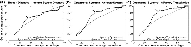
Analysis of KEGG classes coverage by structural cluster regions. Curves associated to the subclass of immune system diseases (a), of sensory systems (b), and olfactory transduction (c). Each arrow corresponds to the point in the curve with largest distance from the corresponding random curve. P-values for these arrow points are . See Supplementary Table S8. Curves are constructed by interpolating on all δ values (see ‘Materials and Methods’ section for the definition of δ steps). Comparison is realized with random curves (dotted curves; see ‘Materials and Methods’ section for randomized gene selection).

An analysis of gene distribution along chromosomes highlighted that genes in a given pathway or in a given subclass are tendentially spread over all chromosomes and over several sites within the same chromosome. Hence, the co-localization of groups of genes and structural clusters becomes a highly unlikely event. For pathways involved in immune systems diseases for instance, one should notice that roughly, the 36% of the entire genome is covered by structural cluster regions and that only a fifth of all structural cluster regions captures the 65% of the genes involved in immune systems diseases (Supplementary Table S9 shows the details of the coverage by structural cluster regions for each chromosome; see Figure 3a). For the asthma pathway (28 genes, ), the 96% of genes are covered by just 10 structural cluster regions distributed over eight chromosomes (when a chromosomal coverage of 40% is considered; Supplementary Table S10). A detailed chromosomal analysis of all subclasses listed in Supplementary Table S3 and of a few more pathways has been reported in Supplementary Tables S9–S28.

Within each KEGG’s subclass, we identified specific pathways explaining the deviation from the random distribution of genes computed for the corresponding subclass. By doing so, we identified several pathways of immune system diseases displaying a strong P-value (like asthma and systemic lupus erythematosus; Supplementary Table S3). Within the sensory system, we identified the olfactory transduction pathway (386 genes) with . See Figures 3c, Supplementary Figures S1–S5 and Supplementary Tables S9–S28 for a detailed analysis of these KEGG’s pathways.

We explored signal transduction pathways. Even though, when taken all together, these pathways do not display a behaviour, which is statistically interesting, when considering them separately, Wnt (150 genes, ), Notch (47 genes, ) and Hedgehog (56 genes, ) display a non-random gene distribution in structural cluster regions (Supplementary Figures S1–S4 and Supplementary Tables S21–S23). These signal transduction pathways were previously pinpointed as prime candidates for miRNA-mediated regulation, and several examples were reported to suggest miRNAs to be generators of graded responses or amplifiers in signal pathways, both for single pathways or signalling cross-talks (59).

Owing to the tendency for structural clusters to be co-localized in regions spanning 1–6 Mb along the chromosomes, we considered non-isolated structural cluster regions (i.e. chromosomal regions containing at least two structural clusters) only and repeated the aforementioned analysis. A slightly larger number of pathways and of subclasses appears to display a non-random distribution of genes within the regions. It is worth noticing that the immune system subclass (801 genes) is now identified with , and that infectious (326 genes) and neurodegenerative (323 genes) diseases subclasses are identified with a . Several new pathways involved in human diseases, metabolism and signal transduction were also found (the complete list is given in Supplementary Table S29; see also Supplementary Figures S2).

Structural clusters and cancer pathways

Several concrete examples of pathways support the hypothesis that miRNAs serve as nodes of signalling networks that ensure homeostasis and regulate cancer, metastasis, fibrosis and stem cell biology (59). We analysed pathways known to be involved in cancer and organized in three different databases, KEGG, ATLAS (39–45) and CGC (46). Similarly to signal transduction pathways, the distributions of cancer genes in these data sets do not display a behaviour, which is sharply distinguishable from random. The three data sets provide comparable results: KEGG displays a cancer gene coverage of 81.84% (for 68.71% coverage of the chromosome) obtained with , ATLAS of 97.78% (92.60%) with and CGC of 81.08% (67.67%) with . By considering each pathway in KEGG separately though, we found that thyroid cancer (29 genes; ; Supplementary Figures S1–S7 and Supplementary Tables S8 and S20) and prostate cancer (89 genes; ; Supplementary Table S29-2) display a non-random gene distribution in structural cluster regions. In particular, ∼10% of thyroid cancer genes are located immediately close (at most one gene separates them) to structural clusters.

Several pathways known to be only indirectly involved in oncogenesis are characterized by genes localized in structural cluster regions defined on non-isolated structural clusters. This is the case for the apoptosis pathway (87 genes, ; Supplementary Figures S1–S4, Supplementary Tables S8 and S25), the Mitogen-Activated Protein Kinase (MAPK) pathway (270 genes; ; Supplementary Table S29-1) and the Vascular Endothelial Growth Factor (VEGF) signalling pathway (75 genes; ). The development of an oncogenic state is a complex process involving the accumulation of multiple independent mutations that lead to deregulation of cell signalling pathways central to the control of cell growth and cell fate (60–62). Our finding is in agreement with this idea and highlights miRNA regulation mechanisms (potentially affected by mutation) as potential causes of signalling pathway disfunctioning.

Structural cluster regions versus fragile sites

A comparison between structural cluster regions and fragile sites, i.e. sites in human chromosomes reporting high genetic instability owing to high mutation rate and frequent deletions or rearrangements in some cancerous cells (63), was made. About 34% of known miRNAs in miRBase v13 are located in fragile sites, and ∼31% lie in structural cluster regions (defined at comparable chromosomal coverage, i.e. ∼26%; see ‘Materials and Methods’ section). Fragile sites and structural cluster regions do not overlap in a meaningful manner: ∼28% of fragile sites only cover structural cluster regions and vice versa (Supplementary Figure S13 and Supplementary Table S30). The comparison between gene distribution for KEGG’s biological pathways within fragile sites and gene distribution within structural cluster regions highlights that structural cluster regions better cover KEGG’s genes (Figure 4). Several large KEGG’s subclasses of human diseases, metabolism and organismal systems are better localized around structural cluster regions than around fragile sites (Supplementary Table S31). At a minor extent, the same holds for genes involved in specific cancer pathways (38.15% versus 33.15%); similar coverages are obtained for ATLAS and CGC data sets (Supplementary Table S32).

Figure 4.

Distribution of gene coverage by fragile sites and by structural cluster regions. Coverage is computed for all biological pathways defined in KEGG and containing at least five genes. Fragile sites cover the 26.38% of chromosomes, and structural cluster regions are set to cover the 26.40%. Structural cluster regions (dotted line) better cover genes in KEGG biological pathways than fragile sites (solid line). See also Supplementary Table S30 and Figure S13.

DISCUSSION

The discovery of structural clusters mir-17-92 (9) and mir-106a-363 (10) involved in cancer development provided the need for a computational tool that helps to characterize potential structural clusters within the human chromosomes as new candidates for experimental tests. An exhaustive naive search of structural clusters cannot be based on a naive sequence search because the computational cost for genomic screening is too high. Based on the observation that structural clusters appear to contain paralogous miRNAs, we could circumvent this problem by designing an algorithm that could search for palindromic regions, therefore for regions that are highly susceptible to contain secondary structures formed by several hairpins, containing paralogous sequences. This intuition allowed us to screen thousands of potential structural clusters and select those that energetically are the most stable and best fit expected combinatorial criteria. Known structural clusters are selected by our system, and together with them, several new ones were predicted. With an a posteriori verification, we remarked several facts that increase the level of confidence in our predictions:

1. The localization of structural clusters in intronic regions versus intergenic regions

2. The identification of known conserved seeds in predicted miRNAs

3. The overrepresentation of miRNA/miRNA* reads within structural clusters predicted from deep-sequencing data

4. The negligeable effect of CDS, exons and ncRNAs filtering of the predictions based on paralogous potential miRNAs (see ‘Materials and Methods’ section)

5. Most structural clusters contain miRNAs targeting some 3′UTR or CDS

6. The regulatory functions of target genes highlighted by 3′UTR and CDS targets functional analysis

7. Functional analysis on miRNAs predicted by paralogous sequences and on by deep-sequencing data taken separately provides comparable results

Our search was realized along the entire human genome, i.e the full genomic sequence including regions, which are highly repeated. We wished to find miRNA structural clusters possibly occurring anywhere along the genome, with the exception of genes. This is because of the evidence that insertion of transposable elements appears to be one of the driving forces that create new miRNAs (64) and that >15% (162 over 1028 non-redundant sequences) of human pre-miRNAs in miRBase v16 are masked by RepeatMasker.

Predictions of structural clusters based on deep-sequencing data are also provided by the algorithm. About a hundred structural clusters were predicted directly from reads, and most of known miRNAs among them are unknown to be organized in clusters. The 86% of them contain miRNAs with known seeds. Their structural organization suggests an organized regulation of the miRNAs occurring in them and might provide an important insight to the biologist. Also, we highlighted 13 new structural clusters whose miRNAs are identified by reads occurring either in cervical cancer or in melanoma and pigment cells experiments (Supplementary Table S7). The miRNAs hosted in these structures are unknown to be structurally organized, and their co-localization might guide the unraveling of their regulatory role.

The rather small overlapping of sets of miRNA structural clusters predicted by the different approaches (Supplementary Figure S3) highlights the interest of combining different algorithmic strategies in the design of predictive tools. As each method optimizes different criteria, the outcomes might vary in terms of miRNA lengths, miRNAs identification within the structural cluster, structural cluster size and so forth. It is worth noticing that a few of our structural clusters are made of very long sequences and contain many miRNAs. The ab initio structural cluster search based on paralogous sequences detected a structural cluster of 26 miRNAs for instance (Supplementary Figure S14), constituted by repeated sequenced that are not known to Repbase (35), by very stable hairpins and by miRNAs with targets. Another example is a 8 miRNA’s structural cluster issued from deep-sequencing data (Supplementary Figure S15), also presenting stable hairpins, miRNAs with targets and very good matching of reads on the miRNA/miRNA* sequences. These cases are rather unique, but they are highlighted to illustrate the strong energy conditions satisfied by the structures as well as the interesting target mapping that is found. Their functionality should be experimentally tested. It has been often argued that new miRNAs are likely to be created by transposable elements generating repeated sequences, and it might be that these two structures are remarkable examples of such process.

Very little is known on the functional implications of the two known miRNA structural clusters, of their potential role in the cross-talking between distinct pathways, on their regulation of a single or multiple target, besides the observation that they are over-expressed in a highly significant manner during cancer. This suggests that miRNA structural clusters can be indicators of regions whose transcription is functionally important during specific conditions, like cancer development, and this was one of the reasons for us to look closer for the content of these regions and in particular to identify the pathways that are co-localized with structural clusters. For instance, the 33% of chromosomal coverage captures 69% of genes involved in thyroid cancer. For this pathway, ∼10% of its genes either contain structural clusters within their introns or they contain them in intergenic regions surrounding them. This strongly suggests that thyroid cancer genes might be regulated by the potential miRNAs contained in the associated structural clusters. Experiments for testing it or in silico gene target identification are required.

The presence of genes associated to important functional subclasses (like immune system diseases, signal transduction, development and sensory system) in structural cluster regions hints for a possible regulation of these genes by miRNAs contained in structural clusters, but this hypothesis deserves an experimental analysis. In particular, the presence of structural clusters within introns of known genes suggests that these structural clusters might be regulated by the promoter of their host gene. One expects, as in the case of mir-17 and c-Myc, to find miRNAs in the cluster regulating (possibly negatively) some of the genes targeted by the activating transcription factor. Finding transcription factors that activate the expression of structural clusters is a direction of investigation to be undertaken.

The strong bias in co-localization between genes of some pathway and structural clusters suggests using structural clusters as genetic landmarks for the prediction of putative genes involved in a pathway. Predictions could be realized by targeting genes involved in the same miRNA regulation or by identifying genes localized within the same structural cluster regions (see Table 5). In the specific case of cancer, predictions of pathway deregulation in cell lines have been shown them to be sensitive to therapeutic agents that target components of the pathway (65). Therefore, a systematic identification of pathways, which are most susceptible to miRNA regulation might turn out to be relevant in the design of therapeutic strategies and drugs.

SUPPLEMENTARY DATA

Supplementary Data are available at NAR Online: Supplementary Tables 1–32, Supplementary Figures 1–15 and Supplementary Data Sets 1–6.

FUNDING

Ministère de l'Enseignement Supérieure et de la Recherche (MESR) doctoral fellowship and a MESR teaching assistantship (to A.M.). Funding for open access charge: Université Pierre et Marie Curie (UPMC), Annual funding from our main institutions: Centre Nationale de la Recherche Scientifique (CNRS) and UPMC.

Conflict of interest statement. None declared.

REFERENCES

- 1.Sempere L, Cole C, McPeek M, Peterson K. The phylogenetic distribution of metazoan microRNAs: Insights into evolutionary complexity and constraint. J. Exp. Zool. B. Mol. Dev. Evol. 2006;306B:575–588. doi: 10.1002/jez.b.21118. [DOI] [PubMed] [Google Scholar]
- 2.Bartel D, Chen C. Micromanagers of gene expression: the potentially widespread influence of metazoan microRNAs. Nat. Rev. Genet. 2004;5:396–400. doi: 10.1038/nrg1328. [DOI] [PubMed] [Google Scholar]
- 3.Bentwich I, Avniel A, Karov Y, Aharonov R, Gilad S, Barad O, Barzilai A, Einat P, Einav U, Meiri E, et al. Identification of hundreds of conserved and nonconserved human microRNAs. Nat. Genet. 2005;37:766–770. doi: 10.1038/ng1590. [DOI] [PubMed] [Google Scholar]
- 4.Bartel D. MicroRNAs: target recognition and regulatory functions. Cell. 2009;1:215–233. doi: 10.1016/j.cell.2009.01.002. [DOI] [PMC free article] [PubMed] [Google Scholar]
- 5.Lewis B, Burge C, Bartel D. Conserved seed pairing, often flanked by adenosines, indicates that thousands of human genes are microRNA targets. Cell. 2005;120:15–20. doi: 10.1016/j.cell.2004.12.035. [DOI] [PubMed] [Google Scholar]
- 6.Friedman R, Farh K, Burge C, Bartel D. Most mammalian mRNAs are conserved targets of microRNAs. Genome Res. 2009;19:92–105. doi: 10.1101/gr.082701.108. [DOI] [PMC free article] [PubMed] [Google Scholar]
- 7.Altuvia Y, Landgraf P, Lithwick G, Elefant N, Pfeffer S, Aravin A, Brownstein MJ, Tuschl T, Margalit H, et al. Clustering and conservation patterns of human microRNAs. Nucleic Acids Res. 2005;33:2697–2706. doi: 10.1093/nar/gki567. [DOI] [PMC free article] [PubMed] [Google Scholar]
- 8.Yu J, Wang F, Yanga G, Wanga F, Maa YN, Zhang JW. Human microRNAs clusters: Genomic organization and expression profile in leukemia cell lines. Biochem. Biophys. Res. Commun. 2006;349:59–68. doi: 10.1016/j.bbrc.2006.07.207. [DOI] [PubMed] [Google Scholar]
- 9.Hayashita Y, Osada H, Tatematsu Y, Yamada H, Yanagisawa K, Tomida S, Yatabe Y, Kawahara K, Sekido Y, Takahashi T. A polycistronic miRNA cluster, miR-17-92, is overexpressed in human lung cancers and enhances cell proliferation. Cancer Res. 2005;65:9628–9632. doi: 10.1158/0008-5472.CAN-05-2352. [DOI] [PubMed] [Google Scholar]
- 10.Landais S, Landry S, Legault P, Rassart E. Oncogenic potential of the miR-106-363 cluster and its implication in human t-cell leukemia. Cancer Res. 2007;67:5699–5707. doi: 10.1158/0008-5472.CAN-06-4478. [DOI] [PubMed] [Google Scholar]
- 11.Mattie M. microRNAs in Cancer (’oncomirs’) In: Clark N, Sanseau P, editors. MicroRNAs: Biology, Function and Expression. Washington, DC: DNA press; 2007. pp. 251–279. [Google Scholar]
- 12.Sewer A, Paul N, Landgraf P, Aravin A, Pfeffer S, Brownstein MJ, Tuschl T, van Nimwegen E, Zavolan M. Identification of clustered microRNAs using an ab initio prediction method. BMC Bioinformatics. 2005;6:267. doi: 10.1186/1471-2105-6-267. [DOI] [PMC free article] [PubMed] [Google Scholar]
- 13.Mathelier A, Carbone A. MIReNA: finding microRNAs with high accuracy and no learning at genome scale and from deep sequencing data. Bioinformatics. 2010;6:2226–2234. doi: 10.1093/bioinformatics/btq329. [DOI] [PubMed] [Google Scholar]
- 14.Abrouka M, Zhanga R, Murata F, Lib A, Ponta C, Mao L, Salse J. Grass microRNA gene paleohistory unveils new insights into gene dosage balance in subgenome partitioning after whole-genome duplication. Plant Cell. 2012;24:1776–1792. doi: 10.1105/tpc.112.095752. [DOI] [PMC free article] [PubMed] [Google Scholar]
- 15.Li Y, Zhang Z, Liu F, Vongsangnak W, Jing Q, Shen B. Performance comparison and evaluation of software tools for microRNA deep-sequencing data analysis. Nucleic Acids Res. 2012;40:4298–4305. doi: 10.1093/nar/gks043. [DOI] [PMC free article] [PubMed] [Google Scholar]
- 16.He L, Thomson J, Hemann M, Hernando-Monge E, Mu D, Goodson S, Powers S, Cordon-Cardo C, Lowe SW, Hannon GJ, et al. A microRNA polycistron as a potential human oncogene. Nature. 2005;435:828–833. doi: 10.1038/nature03552. [DOI] [PMC free article] [PubMed] [Google Scholar]
- 17.O’Donnell K, Wentzel E, Zeller K, Dang C, Mendell J. c-Myc-regulated microRNAs modulate E2F1 expression. Nature. 2005;435:839–843. doi: 10.1038/nature03677. [DOI] [PubMed] [Google Scholar]
- 18.Zhang B, Pan XP, Cox SB, Cobb GP, Anderson TA. Evidence that miRNAs are different from others RNAs. Cell Mol. Life Sci. 2006;63:246–254. doi: 10.1007/s00018-005-5467-7. [DOI] [PMC free article] [PubMed] [Google Scholar]
- 19.Delisi C, Crothers D. Prediction of RNA secondary structure. PNAS. 1971;68:2682–2685. doi: 10.1073/pnas.68.11.2682. [DOI] [PMC free article] [PubMed] [Google Scholar]
- 20.Tinoco I, Uhlenbeck OC, Levine MD. Estimation of secondary structure in ribonucleic acids. Nature. 1971;230:362–367. doi: 10.1038/230362a0. [DOI] [PubMed] [Google Scholar]
- 21.Hofacker I, Fontana W, Stadler P, Bonhoeffer L, Tacker M, Schuster P. Fast folding and comparison of RNA secondary structure. Monatsh. Chem. 1994;125:167–168. [Google Scholar]
- 22.Boguski M, Lowe T, Tolstoshev C. dbEST, database for ’expressed sequence tags’. Nat. Genet. 1993;4:332–333. doi: 10.1038/ng0893-332. [DOI] [PubMed] [Google Scholar]
- 23.Griffith-Jones S. The miRNA registry. Nucleic Acids Res. 2004;32:D109–D111. doi: 10.1093/nar/gkh023. [DOI] [PMC free article] [PubMed] [Google Scholar]
- 24.Griffith-Jones S, Grocock R, van Dongen S, Bateman A, Enright A. miRBase: microRNA sequences, targets and gene nomenclature. Nucleic Acids Res. 2006;34:D140–D144. doi: 10.1093/nar/gkj112. [DOI] [PMC free article] [PubMed] [Google Scholar]
- 25.Griffith-Jones S, Saint H, van Dongen S, Enright A. miRBase: tools for microRNA genomics. Nucleic Acids Res. 2008;36:D154–D158. doi: 10.1093/nar/gkm952. [DOI] [PMC free article] [PubMed] [Google Scholar]
- 26.Gotoh O. An improved algorithm for matching biological sequences. J. Mol. Biol. 1982;162:705–708. doi: 10.1016/0022-2836(82)90398-9. [DOI] [PubMed] [Google Scholar]
- 27.Myers G. A fast bit-vector algorithm for approximate string matching based on dynamic programming. J. ACM. 1999;46:395–415. [Google Scholar]
- 28.Levenshtein V. Binary codes capable of correcting deletions, insertions, and reversals. Sov. Phys. Dokl. 1966;10:707–710. [Google Scholar]
- 29.Emde AK, Grunert M, Weese D, Reinert K, Sperling S. MicroRazerS - rapid alignment of small RNA reads. Bioinformatics. 2010;26:123–124. doi: 10.1093/bioinformatics/btp601. [DOI] [PubMed] [Google Scholar]
- 30.Enright A, John B, Gaul U, Tuschl T, Sander C, Marks DS. MicroRNA targets in Drosophila. Genome Biol. 2003;5:R1. doi: 10.1186/gb-2003-5-1-r1. [DOI] [PMC free article] [PubMed] [Google Scholar]
- 31.John B, Enright A, Aravin A, Tuschl T, Sander C, Marks DS. Human microRNA targets. PLoS Biol. 2005;3:e264. doi: 10.1371/journal.pbio.0020363. [DOI] [PMC free article] [PubMed] [Google Scholar]
- 32.Kertesz M, Iovino N, Unnerstall U, Gaul U, Segal E. The role of site accessibility in microRNA target recognition. Nat. Genet. 2007;39:1278–1284. doi: 10.1038/ng2135. [DOI] [PubMed] [Google Scholar]
- 33.Huang D, Sherman B, Lempicki R. Systematic and integrative analysis of large gene lists using DAVID bioinformatics resources. Nat. Protoc. 2009;4:44–57. doi: 10.1038/nprot.2008.211. [DOI] [PubMed] [Google Scholar]
- 34.Huang D, Sherman B, Lempicki R. Bioinformatics enrichment tools: paths toward the comprehensive functional analysis of large gene lists. Nucleic Acids Res. 2009;37:1–13. doi: 10.1093/nar/gkn923. [DOI] [PMC free article] [PubMed] [Google Scholar]
- 35.Jurka J, Kapitonov VV, Pavlicek A, Klonowski P, Kohany O, Walichiewicz J. Repbase update, a database of eukaryotic repetitive elements. Cyrogenet. Genome Res. 2005;110:462467. doi: 10.1159/000084979. [DOI] [PubMed] [Google Scholar]
- 36.Büttel I, Fechter A, Schwab M. Common fragile sites and cancer: targeted cloning by insertional mutagenesis. Ann. NY. Acad. Sci. 2004;1028:14–27. doi: 10.1196/annals.1322.002. [DOI] [PubMed] [Google Scholar]
- 37.Kanehisa M, Goto S, Hattori M, Aoki-Kinoshita K, Itoh M, Kawashima S, Katayama T, Araki M, Hirakawa M. From genomics to chemical genomics: new developments in KEGG. Nucleic Acids Res. 2006;34:D354–D357. doi: 10.1093/nar/gkj102. [DOI] [PMC free article] [PubMed] [Google Scholar]
- 38.Kanehisa M, Goto S, Kawashima S, Okuno Y, Hattori M. The KEGG resource for deciphering the genome. Nucleic Acids Res. 2004;32:D277–D280. doi: 10.1093/nar/gkh063. [DOI] [PMC free article] [PubMed] [Google Scholar]
- 39.Dorkeld F, Bernheim A, Dessen P, Huret J. A database on cytogenetics in haematology and oncology. Trends Microbiol. 1999;4:214–216. doi: 10.1093/nar/27.1.353. [DOI] [PMC free article] [PubMed] [Google Scholar]
- 40.Huret J, Minor S, Dorkeld F, Bernheim A. Atlas of genetics and cytogenetics in oncology and haematology, an interactive database. Nucleic Acids Res. 2000;28:349–351. doi: 10.1093/nar/28.1.349. [DOI] [PMC free article] [PubMed] [Google Scholar]
- 41.Huret J, Dessen P, Bernheim A. Atlas of genetics and cytogenetics in oncology and haematology, updated. Nucleic Acids Res. 2001;29:303–304. doi: 10.1093/nar/29.1.303. [DOI] [PMC free article] [PubMed] [Google Scholar]
- 42.Pearson H. Lifelines: browsing the cancer catalogue. Nature News. 2001 doi:10.1038/news010531-8. [Google Scholar]
- 43.Kaiser J. Fingerprinting a killer. Science. 2001;292:1803. [Google Scholar]
- 44.Huret J, Dessen P, Bernheim A. Atlas of genetics and cytogenetics in oncology and haematology, year 2003. Nucleic Acids Res. 2003;31:272–274. doi: 10.1093/nar/gkg126. [DOI] [PMC free article] [PubMed] [Google Scholar]
- 45.Huret J, Dessen P, Bernheim A. An internet database on genetics in oncology. Oncogene. 2003;22:1907. [Google Scholar]
- 46.Futreal P, Coin L, Marshall M, Down T, Hubbard T, et al. A census of human cancer genes. Nat. Rev. Cancer. 2004;4:177–183. doi: 10.1038/nrc1299. [DOI] [PMC free article] [PubMed] [Google Scholar]
- 47.Rodriguez A, Griffiths-Jones S, Ashurst J, Bradley A. Identification of mammalian microRNA host genes and transcription units. Genome Res. 2004;14:1902–1910. doi: 10.1101/gr.2722704. [DOI] [PMC free article] [PubMed] [Google Scholar]
- 48.Golan D, Levy C, Friedman B, Shomron N. Biased hosting of intronic microRNA genes. Bioinformatics. 2010;26:992–995. doi: 10.1093/bioinformatics/btq077. [DOI] [PubMed] [Google Scholar]
- 49.Kim YK, Kim V. Processing of intronic microRNAs. EMBO J. 2007;26:775–783. doi: 10.1038/sj.emboj.7601512. [DOI] [PMC free article] [PubMed] [Google Scholar]
- 50.Lewis B, Shih I, Jones-Rhoades M, Bartel D, Burge C. Prediction of mammalian microRNA targets. Cell. 2003;115:787–798. doi: 10.1016/s0092-8674(03)01018-3. [DOI] [PubMed] [Google Scholar]
- 51.Yang JS, Phillips M, Betel D, Mu P, Ventura A, Siepel AC, Chen KC, Lai EC. Widespread regulatory activity of vertebrate microRNA* species. RNA. 2011;17:312–326. doi: 10.1261/rna.2537911. [DOI] [PMC free article] [PubMed] [Google Scholar]
- 52.Czech B, Hannon G. Small RNA sorting: matchmaking for Argonautes. Nat. Rev. Genet. 2011;12:19–31. doi: 10.1038/nrg2916. [DOI] [PMC free article] [PubMed] [Google Scholar]
- 53.Griffiths-Jones S, Hui J, Marco A, Ronshaugen M. MicroRNA evolution by arm switching. EMBO Rep. 2011;12:172–177. doi: 10.1038/embor.2010.191. [DOI] [PMC free article] [PubMed] [Google Scholar]
- 54.Ro S, Park C, Young D, Sanders K, Yan W. Tissue-dependent paired expression of miRNAs. Nucleic Acids Res. 2007;35:5944–5953. doi: 10.1093/nar/gkm641. [DOI] [PMC free article] [PubMed] [Google Scholar]
- 55.Chiang H, Schoenfeld L, Ruby J, Auyeung V, Spies N, Baek D, Johnston WK, Russ C, Luo S, Babiarz JE, et al. Mammalian microRNAs: experimental evaluation of novel and previously annotated genes. Genes Dev. 2010;24:992–1009. doi: 10.1101/gad.1884710. [DOI] [PMC free article] [PubMed] [Google Scholar]
- 56.Li S, Liao Y, Ho M, Tsai K, Lai C, Lin WC. miRNA arm selection and isomiR distribution in gastric cancer. BMC Genomics. 2012;13:S13. doi: 10.1186/1471-2164-13-S1-S13. [DOI] [PMC free article] [PubMed] [Google Scholar]
- 57.Li S, Tsai K, Pan H, Jeng Y, Ho M, Li WH. MicroRNA 3′ end nucleotide modification patterns and arm selection preference in liver tissues. BMC Syst. Biol. 2012;6:S14. doi: 10.1186/1752-0509-6-S2-S14. [DOI] [PMC free article] [PubMed] [Google Scholar]
- 58.Tay Y, Zhang J, Thomson A, Lim B, Rigoutsos I. MicroRNAs to Nanog, Oct4 and Sox2 coding regions modulate embryonic stem cell differentiation. Nature. 2008;455:1124–1128. doi: 10.1038/nature07299. [DOI] [PubMed] [Google Scholar]
- 59.Inui M, Martello G, Piccolo S. MicroRNA control of signal transduction. Nat. Rev. Mol. Cell. Biol. 2010;11:252–263. doi: 10.1038/nrm2868. [DOI] [PubMed] [Google Scholar]
- 60.Fearon E, Vogelstein B. A genetic model for colorectal tumorigenesis. Cell. 1990;17:671–674. doi: 10.1016/0092-8674(90)90186-i. [DOI] [PubMed] [Google Scholar]
- 61.Hanahan D, Weinberg R. The hallmarks of cancer. Cell. 2000;100:57–70. doi: 10.1016/s0092-8674(00)81683-9. [DOI] [PubMed] [Google Scholar]
- 62.Sherr C. Cancer cell cycles. Science. 1996;274:1672–1677. doi: 10.1126/science.274.5293.1672. [DOI] [PubMed] [Google Scholar]
- 63.Glover T. Common fragile sites. Cancer Lett. 2006;232:4–42. doi: 10.1016/j.canlet.2005.08.032. [DOI] [PubMed] [Google Scholar]
- 64.Smalheiser N, Torvik V. Mammalian microRNAs derived from genomic repeats. TRENDS Genet. 2005;21:322–326. doi: 10.1016/j.tig.2005.04.008. [DOI] [PubMed] [Google Scholar]
- 65.Bild A, Yao G, Chang JT, Wang Q, Potti A, Chasse D, Joshi MB, Harpole D, Lancaster JM, Berchuck A, et al. Oncogenic pathway signatures in human cancers as a guide to targeted therapies. Nature. 2006;439:353–357. doi: 10.1038/nature04296. [DOI] [PubMed] [Google Scholar]
Associated Data
This section collects any data citations, data availability statements, or supplementary materials included in this article.