The effect of CT scanner parameters and 3D volume rendering techniques on the accuracy of linear, angular, and volumetric measurements of the mandible

Abstract

Objectives

This study investigates the effect of scanning parameters on the accuracy of measurements from three-dimensional multi-detector computed tomography (3D-CT) mandible renderings. A broader range of acceptable parameters can increase the availability of CT studies for retrospective analysis.

Study Design

Three human mandibles and a phantom object were scanned using 18 combinations of slice thickness, field of view, and reconstruction algorithm and three different threshold-based segmentations. Measurements of 3D-CT models and specimens were compared.

Results

Linear and angular measurements were accurate, irrespective of scanner parameters or rendering technique. Volume measurements were accurate with a slice thickness of 1.25 mm, but not 2.5 mm. Surface area measurements were consistently inflated.

Conclusions

Linear, angular and volumetric measurements of mandible 3D-CT models can be confidently obtained from a range of parameters and rendering techniques. Slice thickness is the primary factor affecting volume measurements. These findings should also apply to 3D rendering using cone-beam-CT.

INTRODUCTION

Three-dimensional computed tomography (3D-CT) is increasingly utilized in clinical and research settings to qualitatively and quantitatively characterize normal and abnormal anatomic structures. There has been an ever-growing need to perform three-dimensional (3D) CT imaging of the mandible or maxilla with conventional multi-detector (MDCT) or cone-beam (CBCT) systems. The development of CBCT has significantly increased the clinical applications of 3D imaging since CBCT can be acquired outside the environment of a conventional MDCT imaging suite while offering lower patient radiation exposure. For example, 3D-CBCT has been used to assess changes in the mandible after orthognathic surgery for mandibular advancement or setback procedures¹; to evaluate screw placement and fracture alignment during fracture reduction or orthognatic surgery^2–3 and to develop clinical applications for dental^4–5 and craniofacial imaging^6–7. Conventional MDCT continues to be routinely used in most institutions to evaluate patients with mandibulomaxillary trauma, sinonasal inflammatory disease, developmental conditions (e.g., midface and mandibular hypoplasia), and neoplastic conditions of the oral cavity, maxilla, and mandible.

Despite these documented 3D applications of conventional MDCT and CBCT, there has been no systematic assessment of the specific CT image acquisition parameters⁸ as well as the 3D reconstruction techniques⁹ that will provide the most accurate linear, angular, volumetric, and surface area measurements. Assessments of 3D-CT renderings (MDCT or CBCT) using human body parts, bony remains, phantom objects, and anatomical models have consistently found linear measurements to be statistically accurate, irrespective of CT acquisition parameters^10–20. Alimited number of studies comparing CBCT and MDCT have focused on linear measurements, using mostly CT series with manufacturers' recommended scanning parameters^{9, 18, 21}. Studies examining volumetric measurements are even rarer²². Thus, there is a definite need to systematically extend assessment of scanner parameters and 3D rendering techniques to include angular, volumetric, and surface area measurements from 3D rendered models.

It is important to determine the scanner parameters and the 3D rendering techniques that yield a comprehensive set of accurate anatomic measurements to ensure optimal patient management. Such information will also aid research efforts to collect and establish normative data of structures such as the mandible by tapping into rich databases of extant imaging studies acquired for different medical reasons. At present, such use of existing imaging studies in medical records is of questionable validity because the images were acquired using scanner parameters that may not be optimal for visualizing specific structures.

With the overall goal of broadening the application of CT studies to render 3D-CT models for diagnostic and research purposes using extant imaging studies^23–25, the purpose of this study is to assess the effect of varying MDCT scanner parameters to determine those acceptable for quantitative 3D modeling for pre- and post-surgical¹⁶ planning; constructing accurate prosthetic material; recognizing treatment change with greater accuracy^{8, 19, 26–27}; monitoring normal growth and development, and establishing normative data. More specifically, this study examines a range of CT scanner parameters typically used for oral treatment to determine the optimal MDCT image acquisition parameters and 3D-CT rendering techniques for securing accurate linear, angular, volumetric, and surface area measurements of the mandible and are representative of anatomic truth, or reference standard, measurements.

MATERIALS AND METHODS

Materials

Figure 1 displays the three mandible specimens and the phantom object scanned in this study. The mandibles (one child and two adult) were secured from the Anatomy Department at the University of Wisconsin-Madison, where they had been dried and prepared. The phantom object, an acrylic prism made of a synthetic polymer (Polymethyl 2-methylpropenoate), had easily-defined edges and was used to confirm methodology of landmarking and measuring the mandibles as described below.

Figure 1.

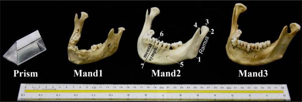
Specimens scanned: Glass prism, Mand1-Child, Mand2-Adult, and Mand3-Adult. Mand2 is labeled to reflect anatomic landmarks listed in Table 1: 1) Gonion, 2) Condyle Lateral, 3) Condyle Superior, 4) Coronoid Process, 5) Mental Foramen, 6) Dental Border Posterior-on Lingual aspect, and 7) Gnathion. The mental symphysis and ramus are also labeled.

Landmarks

Landmarks needed to define the various measurements were determined for both the mandibles (Figure 2) and the prism. The mandibular landmarks placed on the 3D-CT rendered models are depicted as circular nodes (Figure 2, Table 1). All linear and angular measurements, using the predetermined landmarks, are listed in Table 2. The prism's landmarks were its clearly defined edges, corners, and planes. An experienced researcher placed all landmarks.

Figure 2.

Landmark and measurement definitions displayed on the 3D-CT gradient-shaded rendered model of Mand3 in three views (2A) inferior (2B) posterior, and 2(C) left lateral. Landmarks are depicted as bordered circles and measurements as black lines.

Table 1.

Mandibular landmarks are defined with numbers corresponding to labels on Figure 1. Landmark abbreviations include structure name, orientation, and aspect/direction.

Landmark	Side	Abbreviation	Description. See Figure 2 (A, B, or C)
1. Gonion	Left	GoLt	Intersection of planes of the ramus and the mandibular base. (C)
	Right	GoRt
2. Condyle Lateral	Left	CdLaLt	Most superolateral point of the condyle. (B)
	Right	CdLaRt
3. Condyle Superior	Left	CdSuLt	Most superior point of the condylar head. (B)
	Right	CdSuRt
4. Coronoid Process	Left	CoLt	Most superior point of the coronoid process. (C)
	Right	CoRt
5. Mental Foramen	Left	MefLt	Point on mandibular base directly inferior to the mental foramen. (A)
	Right	MefRt
6. Dental Border-Posterior	Central	DbPo	Most superior alveolar bone of dorsal symphysis below the incisor. (B)
7. Gnathion	Central	Gn	Most inferior point on the mental symphysis. (C)

Table 2.

List of linear and angular mandibule measurements with definitions. Measurements are defined by landmark abbreviations as specified in Table 1.

Measurement	Aspect	Abbreviation	Definition: Measurement best visualized in Figure 2 (A, B, or C)
Mandible Angle	Left	∠ CdLaLt-GoLt-Gn	Angle between CdLaLt-GoLt and GoLt-Gn in degrees. (2C)
	Right	∠ CdLaRt-GoRt-Gn
Mandible Length	Left	GoLt-MefLt +MefLt-Gn	Summed distance between gonion, mental foramen-base, and gnathion. (2A)
	Right	GoRt-MefRt +MefRt-Gn
Ramus Depth	Left	CdSuLt-GoLt	Straight, linear distance between the condyle lateral and the gonion. (2B)
	Right	CdSuRt-GoRt
Coronoid Width	Left-Right	CoLt-CoRt	Straight, linear distance between left and right coronoid processes. (2B)
Gonion Width	Left-Right	GoLt-GoRt	Straight, linear distance between left and right gonions. (2A)
Lateral Condyle Width	Left-Right	CdLaLt-CdLaRt	Straight, maximal linear distance between lateral condylar heads. (2B)
Mental Depth	Central	DbPo-Gn	Straight, linear distance between gnathion and posterior dental border. (2B)

Reference Standard Measurements

Measurements representative of the anatomic reference standard (linear, angular, volume, and regional surface area) were obtained directly from the dry mandible specimens and the prism and compared to measurements from their respective 3D-CT models (Table 2). The same researcher measured the dry mandibles and the prism on three different dates, each one week apart, using an electronic digital caliper with an LED display (KURT Precision Instruments, Minneapolis, MN; resolution ± 0.01 mm) and a digital angle rule (GemRed, Guilin, Guangxi, China; ± 0.3° accuracy). The mean of the three measurements was used as the reference standard, against which all software-generated measurements from the 3D rendered models were compared (Table 3).

Table 3.

Anatomic reference standard measurements: The mean±standard deviation for the eight linear measurements (in mm), two angular measurements (in degrees), volume (in cm³) and regional surface area (in cm²).

Measurement Type	Mand1-Child	Mand2-Adult-NoMolar	Mand3-Adult-NoIncisor
Linear Measurements
Mandible Angle - Left	109.38±0.68	121.30±0.43	110.10±0.61
Right	111.27±0.64	119.30±2.35	108.62±1.26
Mandible Length - Left	71.72±0.08	81.73±0.44	79.68±1.56
Right	72.43±1.71	86.75±1.00	80.64±1.17
Ramus Depth - Left	44.57±0.40	55.55±0.13	58.82±0.40
Right	44.90±0.39	55.32±0.59	60.34±0.33
Coronoid Width	73.35±0.30	96.29±0.30	92.23±1.67
Gonion Width	71.75±0.35	98.28±0.25	91.26±0.16
Lateral Condyle Width	88.96±0.32	109.80±0.44	118.59±1.70
Mental Depth	23.83±0.41	33.32±0.24	31.91±0.18
Volume	42.23±2.75	74.17±4.25	70.60±1.50
Regional Surface Area	41.17±1.89	44.20±6.56	54.11±1.94

Volumes of the mandibles and prism were established by three separate water displacement trials, where each mandible was covered with a thin layer of an adhesive plastic sheet (to prevent water seepage into the alveolar bone and foramen and hence minimize the potential of underestimating water volume displaced on subsequent trials), and then submerged in water. Water displacement was measured with a calibrated 25 ml graduated cylinder for a total of three trials per mandible, and the mean of the three measurements was used as the reference standard. Due to the irregular shape of the mandible, the reference standard for surface area was limited to a defined triangular region on the lateral side of the mandible defined by three measurement landmarks (Gn, GoLt, CdLaLt), shown on Figure 2 and defined in Table 1. Surface area was measured by applying clear graph paper along the curvature of the mandible specimens and calculating its area. The total surface area of the prism was calculated directly using the digital calipers. As described above, the mean of three surface area measurements was used as the reference standard for the mandible, and for the prism.

Image Acquisition

The three mandibles and the prism were scanned using a General Electric LightSpeed 16 MDCT scanner (General Electric Medical Systems, Milwaukee, WI) with a tube voltage of 120 kV and an effective tube current of 105.0 mAs. The beam collimation was 10 × 0.625 mm. All mandible CT scans were acquired with a 512 × 512 mm matrix, and using scanner parameters in 18 combinations of reconstruction algorithm, field of view (FOV), and slice thickness as specified in the next paragraph. All images were saved in DICOM format for the subsequent step of loading the different image series into Analyze^® 10.0 (AnalyzeDirect^®, Overland Park, KS, USA) for 3D rendering. The mandibles and the prism were scanned in 1.5L of water to provide soft tissue equivalent attenuation and to provide a baseline to quantify the reconstruction process, since water measures at zero Hounsfield Units (HU).

The image acquisition plane traveled from the mental symphysis to the condyles (see Figure 1). The mandibles were not sealed during scanning, as water density inside the mandible more closely simulates the density of living human mandibles. The following scanner parameters and variables were used: a) Reconstruction algorithm using the three options available (Soft, Standard, BonePlus), since algorithm greatly affects the quality of tissue detail and has been reported to alter the volume measurements of 3D models of phantom objects^28–29; b) FOV set at: 16×16cm, 18×18cm, or 30×30 cm, since FOV directly defines pixel size and in-plane image resolution, which can affect volume measurements; and c) Slice thickness of either 1.25 mm or 2.5 mm to determine whether image series with these slice thicknesses will yield accurate volume-averaging.

The prism, with its clearly defined borders and smooth surface, was scanned with the same CT scanner as the mandibles to authenticate this study's protocol for linear, angular, volumetric, and surface area measurements. However, scanning parameters more appropriate to its size and density were used and included: slice thicknesses of 0.625mm, 1.25mm, and 2.5mm; FOV 14×14; and two reconstruction algorithms (standard and BonePlus, since the prism is of uniform and homogeneous density greater than the range of soft tissue). Also, only a single FOV was used, since measurements from the three FOVs used for mandible 3D-CT renderings revealed no significant differences (ANOVA [F(2, 51) = 0.012, p = 0.988]), a finding similar to those of Ravenel et al³⁰.

Rendering 3D Segmented Models

Each series was rendered as 3D computer models in the software package Analyze 10.0^® by applying two rendering techniques: Volume Render (VR) and Volume of Interest (VOI). VR provides a gradient shaded opaque model from a volume dataset with clear surface detail and three-dimensional relationships⁹. VOI defines an object surface overlay and assembles the slices into a visual model. VOI was performed by applying an automated segmentation threshold to each DICOM image (VOI-Auto) and was then manipulated manually to define the mandible surface overlay on the images post-thresholding (VOI- Manual). Thus, each series was rendered into 3D-CT computer models using VR, VOI-Auto, and VOI-Manual.

The selection of an appropriate window for threshold-based segmentation on image intensity is essential to modeling as it defines the data available for visualization and measurement. The VR, VOI-Auto, and VOI-Manual models were segmented with a global thresholding range of 150–3071 HU for all three mandibles. The advantage of using a global threshold range is that only one parameter is estimated in segmentation, and when applied to all imaging studies, it eliminates observer-specific threshold values and makes differences in measurement less subject to variation¹⁸. The minimum HU value was at a density level below the density of cortical osseous tissue, but was necessary to encompass the range of cancellous bone for accurate 3D reconstruction³¹ and is the same as that used by Kuszyk et al.⁹. The maximum HU value is the number recommended for optimal 3D-CT measurement accuracy^{12, 31} and met the need to include all voxels representing tooth enamel. This was verified by using the Probe Tool of eFilm^® 3.1.0 (Merge Healthcare, Milwaukee, WI) while viewing the DICOM images. A global threshold range of (50–250HU) was applied to the prism to maximize border alignment of the segmentation process with the DICOM images. This selective thresholding range for the prism gave a more accurate segmentation of the object, allowing landmarking to be done with fewer inherent sources of error.

All three mandibles were rendered in 3D using all experimental combinations of the three reconstruction algorithms (Soft, Standard, and BonePlus), three FOVs, and two slice thicknesses. This yielded 18 CT series of each mandible, with each series rendered under three different techniques (VR, VOI-Auto, and VOI-Manual), amounting to a total of 54 models per mandible and a grand total of 162 mandible models. The prism was scanned with two reconstruction algorithms (Standard and BonePlus), one FOV, and three slice thicknesses, and then rendered in all three techniques for a total of 18 prism models.

3D-CT Model Measurements

The landmarks were digitally placed on each of the mandible models rendered using the Fabricate tool within Analyze^®. This tool displays a four-panel window containing sagittal, axial, and coronal reconstruction views of the DICOM data in addition to the corresponding model. The digital landmark placement protocol improves measurement accuracy by an average of 98% as measured by reduction in error variability³². Using the placed landmarks, linear and angular measurements (Table 2) were recorded for each 3D-CT model (n=162). All two-dimensional measurements were taken as the shortest possible distance between landmarks through all spatial planes. The protocol for landmarking and measurement was an adaptation of the methodology of several studies^{10, 17, 31, 33, 34}.

Volume measurements for each rendering were secured as automated calculations within the Sample Options tool of Analyze^®. Regional surface area measurements of the mandible were performed with the Area Measure tool of Analyze^®. The same region that was defined on each of the dry mandible specimens was defined digitally on each model using the pre-defined landmarks (Gn, GoLt, CdLaLt). The prism total surface area was digitally calculated in the Sample Options tool within Region of Interest in Analyze^®.

Statistical Analysis on 3D-CT Model Measurements

To assess the accuracy of 3D-CT measurements, all measurements described above were compared to their respective anatomic reference standards by calculating the average absolute relative error (ARE) as defined b Chung et al.³², using the following formula.

$$\mathit{ARE}=\frac{1}{n}{\Sigma }_{i=0}^n\mid \frac{3\mathrm{DCT}\mathrm{measurement}-\mathrm{reference}\mathrm{standard}}{\mathrm{reference}\mathrm{standard}}\mid$$

The ARE was calculated separately for each rendering technique, and for each of the three scanning parameters. An ARE ≤ 0.05, which reflects the average difference of less than 5% between anatomical and digital measurement and a commonly acceptable standard by most studies^35–37, was considered to be acceptably accurate for this study. Standard deviations of ARE were calculated using the sample standard deviation equation by dividing the sum of squares by one less than the number in the sample.

To assess for statistical significance on measurement differences, the software package for statistical analysis (SPSS, 2010; referred to as Predictive Analytics SoftWare PASW Statistics v. 18.0.2)³⁸ was used to perform either univariate ANOVA for testing three variables simultaneously, or t-test for two variables. This approach follows the framework established by a study on measurement error, to ensure measurement consistency, by Chung et al. (2008)³². To test for volume measurement difference among the three windows of FOV, univariate ANOVA was used. To test for standard reconstruction algorithms against the reference standard, t-test was used.

RESULTS

Measurements were secured from the 3D-CT rendered models specific to the different scanner parameters manipulated (reconstruction algorithm, FOV, and slice thickness), as well as the 3D volume rendering technique (VR, VOI-Auto, VOI-Manual). These measurements were comparatively assessed for each experimental parameter and compared to anatomic reference standard values using ARE and statistical analyses.

When linear and volumetric measurements for the mandibles were separated by field of view, the relative error (shown in Table 4, FOV column) remained within the experimental threshold for accuracy. This implies that FOV in the range typically used for patients does not affect measurements from resultant 3D-CT rendered models as notably as other parameters. Furthermore, there was no significant difference in volume measurement found between the three windows of FOV as tested by univariate ANOVA [F (2, 51) = 0.012; p = 0.988]. Therefore, the prism was scanned with only one FOV to save time in scanning and modeling.

Table 4.

Average relative error (ARE) and standard deviation (SD) for linear and angular measurements (Line & Ang), volume, and surface area (Surf. Area) for rendering techniques and scanner parameters. Each column represents the combined relative errors for all three mandibles from all experimental variables. These averages are separated in group of analysis by the variable listed as the column title. ARE ≤ 0.05 is denoted by boldface italics. See text for additional clarification.

		Rendering Technique			Reconstruction Algorithm			Field of View (FOV)			Slice Thickness
	Specimen	Technique	ARE	(SD)	Algorithm	ARE	(SD)	FOV	ARE	(SD)	Slice mm	ARE	(SD)
Line(cm) & Ang(°)	Mandibles	VR	0.050	(2.48)	Bone	0.034	(2.01)	16×16	0.035	(2.27)	1.25mm	0.036	(2.41)
	Mandibles	VOI-Auto	0.020	(1.13)	Soft	0.035	(2.49)	18×18	0.034	(1.87)	2.5mm	0.032	(1.86)
	Mandibles	VOI-Manual	0.032	(1.38)	Standard	0.031	(1.66)	30×30	0.033	(2.35)
	Prism	VR	0.013	(0.52)	Bone	0.010	(0.55)				0.625mm	0.009	(0.04)
	Prism	VOI-Auto	0.008	(0.48)	Standard	0.009	(0.52)				1.25mm	0.007	(0.28)
	Prism	VOI-Manual	0.007	(0.40)							2.5mm	0.013	(0.54)
Volume (cm3)	Mandibles	VR	0.082	(3.75)	Bone	0.059	(3.68)	16×16	0.081	(3.83)	1.25mm	0.048	(2.64)
	Mandibles	VOI-Auto	0.086	(3.88)	Soft	0.090	(3.10)	18×18	0.080	(3.99)	2.5mm	0.106	(2.73)
	Mandibles	VOI-Manual	0.064	(3.66)	Standard	0.082	(3.14)	30×30	0.069	(3.77)
	Prism	VR	0.007	(237.19)	Bone	0.013	(480.02)				0.625mm	0.021	(1109.41)
	Prism	VOI-Auto	0.052	(1164.71)	Standard	0.037	(1286.47)				1.25mm	0.021	(902.35)
	Prism	VOI-Manual	0.016	(562.93)							2.5mm	0.033	(1086.01)
Surf. Area (cm2)	Mandibles	VR	0.414	(44.19)	Bone	0.390	(27.24)	16×16	0.395	(48.17)	1.25mm	0.417	(52.36)
	Mandibles	VOI-Auto	0.402	(37.85)	Soft	0.452	(54.51)	18×18	0.381	(28.74)	2.5mm	0.397	(29.28)
	Mandibles	VOI-Manual	0.405	(43.13)	Standard	0.380	(32.99)	30×30	0.444	(48.57)
	Prism	VR	0.126	(814.14)	Bone	0.193	(441.66)				0.625mm	0.088	(467.91)
	Prism	VOI-Auto	0.149	(574.81)	Standard	0.041	(170.77)				1.25mm	0.129	(732.38)
	Prism	VOI-Manual	0.077	(377.96)							2.5mm	0.135	(676.62)

Table 4 also shows that the ARE for all linear measurements are ≤ 0.05 for the mandible specimens, and ≤ 0.013 for the prism, irrespective of rendering technique or scanner parameter. This indicates general similarity between 3D-CT linear measurements and reference standards, and is exemplified by the Mand1-Child measurements in Figure 3, with horizontal lines in Figure 3 depicting the reference standards. Even when there is a wide spread for select measurements in the box plot, paired t-test comparisons showed the measurements from 3D models did not differ significantly from the reference standard (ex.VR measurement for LML-left mandible length; p=0.699).

Figure 3.

Linear distance measurements of Mand1-Child from 3D-CT segmented mandible models separated by rendering technique and compared to reference standard values (horizontal solid lines). The measurements include: MD – mental depth, LR – left ramus depth, LML – left mandible length, CW – coronoid width, GW – gonion width, and LCW – lateral condyle width. Box plots show the mean and lower/upper quartiles of data with whiskers representing 5^th and 95^th percentiles. To conserve space and for clarity of this figure, only left-sided measurements are presented, since left- and right-sided results were similar.

The results for volume measurements are summarized in Table 5 and Figure 4. Findings summarized in Table 5 indicate that the VOI-Manual rendering technique produced 3D-CT volumes closest to anatomic reference standards across all three mandibles. This was expected, as any imperfections in border definition from thresholding in VR and Auto-VOI surface overlays were found and user-corrected. VOI-Manual differed significantly from both VOI-Auto and VR only for the case of Mand1-Child [F (2, 34) = 10.763; p = 0.005].

Table 5.

Average relative error (ARE) and standard deviation (SD) of volumetric measurements from all three mandibles, separated by scan slice thickness. Columns represent the cumulative ARE for all experimental manipulations combined, separated by the variable being examined listed as the column title. Measurement ARE ≤ 0.05 are considered within experimental accuracy and are denoted by boldface italics.

		Rendering Technique			Reconstruction Algorithm			Field of View
	Specimen	Technique	ARE	(SD)	Algorithm	ARE	(SD)	FOV	ARE	(SD)
1.25mm	Mandibles	VR	0.048	(2.40)	Bone	0.044	(0.95)	16×16	0.056	(3.02)
	Mandibles	VOI-Auto	0.047	(2.47)	Soft	0.054	(1.51)	18×18	0.049	(2.66)
	Mandibles	VOI-Manual	0.050	(3.06)	Standard	0.047	(1.10)	30×30	0.038	(2.32)
2.5mm	Mandibles	VR	0.116	(2.47)	Bone	0.073	(2.32)	16×16	0.106	(2.69)
	Mandibles	VOI-Auto	0.124	(1.84)	Soft	0.126	(1.06)	18×18	0.111	(2.85)
	Mandibles	VOI-Manual	0.078	(2.72)	Standard	0.118	(2.22)	30×30	0.101	(2.55)

Figure 4.

3D-CT rendered model volumes separated by specimen and scan slice thickness as compared to anatomic reference standard values (horizontal lines). Volumetric measurements using thin CT slices are closer to reference standards than thicker 2.5 mm slices. Box plots show the mean and lower/upper quartiles of data with whiskers representing 5^th and 95^th percentiles.

Volumetric results for the three reconstruction algorithms (BonePlus, Soft, Standard) were also compared to each mandible's anatomic reference standard. As summarized in Table 4, the BonePlus algorithm generally produced the most accurate 3D-CT models across all three mandibles. The Standard and Soft algorithms had inflated volumes for the adult mandibles, most likely due to their poorer image precision and outward distortion of edges. Although the Standard and Soft algorithms did not perform as well as BonePlus, there were mandible-specific results where the Standard reconstruction algorithm did not significantly differ from the reference standard for Mand1-Child using the t-test (t=2.083; p=0.053).

As for volumetric measurements based on imaging slice thickness, only the 1.25 mm slice thickness for the mandibles produced an ARE ≤ 0.05, but the slice thickness parameter did not alter the volumetric measurements of the prism (ARE for each slice thickness = 0.021, 0.021, and 0.033). 3D-CT volumetric measurements using the 1.25 mm slice thickness yielded small AREs irrespective of rendering techniques or other scanner parameters and variables. Closer examination of volumetric ARE (summarized in Table 5), using the 1.25 mm slice thickness revealed that seven of the nine groups produced an ARE ≤ 0.05. The remaining two groups of 1.25 mm data approached this threshold (ARE=0.054 and 0.056). In marked contrast, no groups scanned with 2.5 mm slice thickness produced acceptable measurement accuracy, indicating that the selection of slices 2.5 mm or thicker is likely to result in higher error for volume measurement. These findings indicate that, in general, thinner scan slices yield volumes closer to anatomic reference standards. However, for the prism, a slice thickness of 1.25 mm was as acceptable as a thinner slice of 0.625 mm

Surface area measurements for both the prism and the mandibles exhibited a high degree of relative error and standard deviation irrespective of scanner parameters or rendering techniques, indicating that all surface area measurement were below the acceptable level of accuracy (see Table 3).

DISCUSSION

The primary objective of this study was to determine the range of CT acquisition parameter settings that provide accurate linear, angular, volumetric, and surface area measurements for 3D-CT reconstruction of bony structures like the mandible using different rendering techniques. Linear measurements were shown to be accurate for all scanning parameters examined irrespective of rendering technique. Volume measurements were shown to be accurate for thicker slices (1.25 mm) than normally used for modeling (0.5 – 0.625 mm), but not for slices as thick as 2.5 mm. Surface area measurements did not meet the experimental threshold for accuracy for the parameters examined here.

MDCT was used for evaluation because of its documented high spatial resolution, contrast resolution, and signal-to-noise ratio^{21, 39}. Since 3D-CT is a post-processing technique and the 3D program cannot discriminate whether the source images were obtained on MDCT or CBCT, the factors that improve 3D image quality and measurement accuracy should be identical, as long as the radiation dose is not so low that the signal-to-noise ratio is compromised. Therefore, the acquisition parameters of slice thickness, reconstruction algorithm, and field of view on 3D rendering, as investigated here, should apply equally to CBCT. Given the increasing clinical use of 3D-CBCT imaging, a formal and systematic investigation for -CBCT is warranted, and can be guided by the acquisition parameters used here.

For bony craniofacial structures like the mandible, the manufacturer's suggested scanning parameters –commonly defined as a bony reconstruction algorithm (e.g., BonePlus, B50, B70) and a minimized FOV– produced accurate 3D-CT linear measurements, in agreement with published studies^{10, 12–13, 16–20}, Image acquisition parameters outside the manufacturer's suggested settings for segmentation technique, reconstruction algorithm, FOV, and slice thickness did not measurably alter the accuracy of linear measurements (0.031≤ARE≤0.036).

As has been reported previously, slice thickness had the most profound effect on the accuracy of 3D-CT volume measurements³⁰ . Thinner slices allow less partial volume-averaging through a series and allow greater image quality for detail⁴⁰. For all three rendering techniques, volumetric measurements from 3D-CT renderings were of acceptable accuracy at 1.25 mm slice thickness (0.047≤ARE≤0.050), but not at 2.5 mm. A major purpose of this study was to quantify the acceptability of commonly used thicknesses greater than 0.625 mm. Although 0.625 mm slices are often used clinically, these findings show that 1.25 mm may also be an acceptable slice thickness for 3D rendering of the mandible for volumetric measurement.

In contrast to linear and volume measurements, surface area measurements did not produce acceptable levels of accuracy for the mandibles, and were considerably inflated. The object overlay method to segmentation done in VOI exhibited visible stair-step artifacts around the surfaces of the classified regions, as described by others^{9, 41}, which may contribute to the inflation of measured surface area. It is possible that the thinner slices (<1 mm), like those commonly used for clinical 3D rendering, may reduce surface area measurement errors. As expected, the prism —which lacks the curvature and contour of the mandible— produced surface area measurements closer to its reference standard. but these measurements strayed farther from the anatomic reference standard with increasing slice thickness.

Accurate methodology is critical for measurement reliability and to quantify changes over time. The rigorous protocol used in this study for landmarking ensured the reproducibility of landmark placements and thus the resultant measurements were only minimally influenced by software user error. A limitation of this study is that the findings from a single scanner and volumetry program may not be directly applicable to other scanners, packages, or rendering platforms. More specific acquisition parameters like pitch, scanner current, increment, beam collimation, and additional degrees of reconstruction algorithm may also be investigated for their effect on resultant 3D-CT volume data modeling in future studies. Also, the experimental design did not allow in situ measurements from actual patient mandibles, which may differ from measurements obtained from bony remains. However, a major strength of this study is that the placement of digital landmarks were on 3D-CT renderings instead of physical landmarks affixed to the mandible specimens⁴², This simulates the reality of analyzing patient scans in clinical and research settings, where there are no prepared specimens or pre-identified anatomy⁴³. Also, findings based on scanner parameters should be applicable to CBCT though formal and systematic assessment is warranted.

3D-CT can provide images of the osseous skeleton of the face and mandible. Additional investigations are needed to determine appropriate acquisition parameters and 3D rendering methods for other bony structures in the head and neck region, as well as for structures containing air or soft-tissue components. More universal parameters may make it possible to create acceptably accurate 3D images for research purposes and treatment planning from a wide range of CT scans obtained with different acquisition parameters. Broader parameters would allow retrospective analysis of extant patient images for purposes beyond those of the original scan, such as to establish normative growth data and the relational growth of different structures (e.g. mandible and hyoid bone). This study has contributed to the establishment of a wider range of acceptable acquisition parameters and rendering methods which will enhance the value of 3D-CT in both research and clinical settings.

REFERENCES

- 1.Cevidanes LH, Bailey LJ, Tucker SF, Styner MA, Mol A, Phillips CL, et al. Three-dimensional cone-beam computed tomography for assessment of mandibular changes after orthognathic surgery. Am J Orthod Dentofacial Orthop. 2007;131(1):44–50. doi: 10.1016/j.ajodo.2005.03.029. [DOI] [PMC free article] [PubMed] [Google Scholar]
- 2.Nkenke E, Zachow S, Benz M, Maier T, Veit K, Kramer M, et al. Fusion of computed tomography data and optical 3D images of the dentition for streak artefact correction in the simulation of orthognathic surgery. Dentomaxillofac Radiol. 2004;33:226–32. doi: 10.1259/dmfr/27071199. [DOI] [PubMed] [Google Scholar]
- 3.Pohlenz P, Blessmann M, Blake F, Gbara A, Schmelzle R, Heiland M. Major mandibular surgical procedures as an indication for intraoperative imaging. J Oral Maxillofac Surg. 2008;66(2):324–9. doi: 10.1016/j.joms.2007.03.032. [DOI] [PubMed] [Google Scholar]
- 4.Hashimoto K, Arai Y, Iwai K, Araki M, Kawashima S, Terakado M. A comparison of a new limited cone beam computed tomography machine for dental use with a multidetector row helical CT machine. Oral Surg Oral Med Oral Path Oral Radiol Endod. 2003;95(3):371–377. doi: 10.1067/moe.2003.120. [DOI] [PubMed] [Google Scholar]
- 5.Mozzo P, Procacci C, Tacconi A, Martini PT, Andreis IA. A new volumetric CT machine for dental imaging based on the cone-beam technique: preliminary results. Eur Radiol. 1998;8(9):1558–1564. doi: 10.1007/s003300050586. [DOI] [PubMed] [Google Scholar]
- 6.Mah J, Hatcher D. Three dimensional craniofacial imaging. Am J Orthod Dentofac Orthop. 2004;126(3):308–309. doi: 10.1016/j.ajodo.2004.06.024. [DOI] [PubMed] [Google Scholar]
- 7.Sukovic P. Cone beam computed tomography in craniofacial imaging. Orthod Craniofac Res. 2003;6(suppl 1):31–36. doi: 10.1034/j.1600-0544.2003.259.x. [DOI] [PubMed] [Google Scholar]
- 8.Ringl H, Schernthaner R, Philipp MO, Metz-Schimmerl S, Czerny C, Weber M, et al. Three-dimensional fracture visualisation of multidetector CT of the skull base in trauma patients: comparison of three reconstruction algorithms. Eur Radiol. 2009;19(10):2416–2424. doi: 10.1007/s00330-009-1435-1. [DOI] [PubMed] [Google Scholar]
- 9.Kuszyk BS, Heath DG, Bliss DF, Fishman EK. Skeletal 3-D CT: advantages of volume rendering over surface rendering. Skeletal Radiol. 1996;25(3):207–214. doi: 10.1007/s002560050066. [DOI] [PubMed] [Google Scholar]
- 10.Brown AA, Scarfe WC, Scheetz JP, Silveira AM, Farman AG. Linear accuracy of cone beam CT derived 3D images. Angle Orthod. 2009;79(1):150–157. doi: 10.2319/122407-599.1. [DOI] [PubMed] [Google Scholar]
- 11.Cavalcanti MG, Rocha SS, Vannier MW. Craniofacial measurements based on 3D-CT volume rendering: implications for clinical applications. Dentomaxillofac Radiol. 2004;33(3):170–6. doi: 10.1259/dmfr/13603271. [DOI] [PubMed] [Google Scholar]
- 12.Damstra J, Fourie Z, Huddleston Slater JJR, Ren Y. Accuracy of linear measurements from cone-beam computed tomography-derived surface models of different voxel sizes. Am J Orthod Dentofacial Orthop. 2010;137(1):16, e11–16. doi: 10.1016/j.ajodo.2009.06.016. discussion 16–17. [DOI] [PubMed] [Google Scholar]
- 13.El-Zanaty HM, El-Beialy AR, El-Ezz AMA, Attia KH, El-Bialy AR, Mostafa YA. Three-dimensional dental measurements: An alternative to plaster models. Am J Orthod Dentofacial Orthop. 2010;137(2):259–265. doi: 10.1016/j.ajodo.2008.04.030. [DOI] [PubMed] [Google Scholar]
- 14.Hassan B, Couto Souza P, Jacobs R, De Azambuja Berti S, van der Stelt P. Influence of scanning and reconstruction parameters on quality of three-dimensional surface models of the dental arches from cone beam computed tomography. Clin Oral Investig. 2010;14(3):303–310. doi: 10.1007/s00784-009-0291-3. [DOI] [PMC free article] [PubMed] [Google Scholar]
- 15.Hassan B, van der Stelt P, Sanderink G. Accuracy of three-dimensional measurements obtained from cone beam computed tomography surface-rendered images for cephalometric analysis: influence of patient scanning position. Eur J Orthod. 2009;31(2):129–34. doi: 10.1093/ejo/cjn088. [DOI] [PubMed] [Google Scholar]
- 16.Katsumata A, Fujishita M, Maeda M, Ariji Y, Ariji E, Langlais RP. 3D-CT evaluation of facial asymmetry. Oral Surg Oral Med Oral Pathol Oral Radiol Endod. 2005;99(2):212–220. doi: 10.1016/j.tripleo.2004.06.072. [DOI] [PubMed] [Google Scholar]
- 17.Lagravere MO, Carey J, Toogood RW, Major PW. Three-dimensional accuracy of measurements made with software on cone-beam computed tomography images. Am J Orthod Dentofacial Orthop. 2008;134(1):112–116. doi: 10.1016/j.ajodo.2006.08.024. [DOI] [PubMed] [Google Scholar]
- 18.Loubele M, Maes F, Schutyser F, Marchal G, Jacobs R, Suetens P. Assessment of bone segmentation quality of cone-beam CT versus multislice spiral CT: a pilot study. Oral Surg Oral Med Oral Pathol Oral Radiol Endod. 2006;102(2):225–234. doi: 10.1016/j.tripleo.2005.10.039. [DOI] [PubMed] [Google Scholar]
- 19.Moerenhout BA, Gelaude F, Swennen GRJ, Casselman JW, Van der Sloten J, Mommaerts MY. Accuracy and repeatability of cone-beam computed tomography (CBCT) measurements used in the determination of facial indices in the laboratory setup. J Craniomaxillofac Surg. 2009;37(1):18–23. doi: 10.1016/j.jcms.2008.07.006. [DOI] [PubMed] [Google Scholar]
- 20.Periago DR, Scarfe WC, Moshiri M, Scheetz JP, Silveira AM, Farman AG. Linear accuracy and reliability of cone beam CT derived 3-dimensional images constructed using an orthodontic volumetric rendering program. Angle Orthod. 2008;78(3):387–395. doi: 10.2319/122106-52.1. [DOI] [PubMed] [Google Scholar]
- 21.Liang X, Lambrichts I, Sun Y, Denis K, Hassan B, Li L, et al. A comparative evaluation of Cone Beam Computed Tomography (CBCT) and Multi-Slice CT (MSCT). Part II: On 3D model accuracy. Eur J Radiol. 2010;75(2):270–274. doi: 10.1016/j.ejrad.2009.04.016. [DOI] [PubMed] [Google Scholar]
- 22.Albuquerque MA, Gaia BF, Cavalcanti MG. Comparison between multislice and cone-beam computerized tomography in the volumetric assessment of cleft palate. Oral Surg Oral Med Oral Pathol Oral Radiol Endod. 2011;112(2):249–57. doi: 10.1016/j.tripleo.2011.03.006. [DOI] [PubMed] [Google Scholar]
- 23.Seo S, Chung MK, Whyms BJ, Vorperian HK. Mandible shape modeling using the second eigenfunction of the Laplace-Beltrami operator. Proc SPIE. 2011;79620Z doi:10.1117/12.877537 -conference proceeding. [Google Scholar]
- 24.Vorperian HK, Wang S, Chung MK, Schimek EM, Durtschi RB, Kent RD, et al. Anatomic development of the oral and pharyngeal portions of the vocal tract: An imaging study. J Acoust Soc Am. 2009;125(3):1666–78. doi: 10.1121/1.3075589. [DOI] [PMC free article] [PubMed] [Google Scholar]
- 25.Vorperian HK, Wang S, Schimek EM, Durtschi RB, Kent RD, Gentry LR, et al. Developmental sexual dimorphism of the oral and pharyngeal portions of the vocal tract: An imaging study. J Speech Lang Hear Res. 2011;54(4):995–1010. doi: 10.1044/1092-4388(2010/10-0097). [DOI] [PMC free article] [PubMed] [Google Scholar]
- 26.Alkadhi H, Wildermuth S, Marincek B, Boehm T. Accuracy and time efficiency for the detection of thoracic cage fractures: volume rendering compared with transverse computed tomography images. J Comput Assist Tomogr. 2004;28(3):378–385. doi: 10.1097/00004728-200405000-00013. [DOI] [PubMed] [Google Scholar]
- 27.Philipp MO, Kubin K, Mang T, Hormann M, Metz VM. Three-dimensional volume rendering of multidetector-row CT data: applicable for emergency radiology. Eur J Radiol. 2003;48(1):33–38. doi: 10.1016/s0720-048x(03)00197-9. [DOI] [PubMed] [Google Scholar]
- 28.Shin H, King B, Galanski M, Matthies HK. Use of 2D histograms for volume rendering of multidetector CT data: development of a graphical user interface. Acad Radiol. 2004;11(5):544–550. doi: 10.1016/j.acra.2004.01.013. [DOI] [PubMed] [Google Scholar]
- 29.Tecco S, Saccucci M, Nucera R, Polimeni A, Pagnoni M, Cordasco G, et al. Condylar volume and surface in Caucasian young adult subjects. BMC Med Imaging. 2010;10:28. doi: 10.1186/1471-2342-10-28. [DOI] [PMC free article] [PubMed] [Google Scholar]
- 30.Ravenel JG, Leue WM, Nietert PJ, Miller JV, Taylor KK, Silvestri GA. Pulmonary nodule volume: effects of reconstruction parameters on automated measurements--a phantom study. Radiology. 2008;247(2):400–408. doi: 10.1148/radiol.2472070868. [DOI] [PMC free article] [PubMed] [Google Scholar]
- 31.Schlueter B, Kim KB, Oliver D, Sortiropolous G. Cone Beam Computed Tomography 3D Reconstruction of the Mandibular Condyle. The Angle Orthodontist. 2008;78(5):880–888. doi: 10.2319/072007-339.1. [DOI] [PubMed] [Google Scholar]
- 32.Chung D, Chung MK, Durtschi RB, Vorperian HK. Determining length-based measurement consistency from magnetic resonance images. Acad Radiol. 2008;15:1322–1330. doi: 10.1016/j.acra.2008.04.020. [DOI] [PMC free article] [PubMed] [Google Scholar]
- 33.Krarup S, Darvann TA, Larsen P, Marsh JL, Kreiborg S. Three-dimensional analysis of mandibular growth and tooth eruption. J Anat. 2005;207(5):669–682. doi: 10.1111/j.1469-7580.2005.00479.x. [DOI] [PMC free article] [PubMed] [Google Scholar]
- 34.Williams FL, Richtsmeier JT. Comparison of mandibular landmarks from computed tomography and 3D digitizer data. Clin Anat. 2003;16(6):494–500. doi: 10.1002/ca.10095. [DOI] [PubMed] [Google Scholar]
- 35.Hammerle CHF, Wagner D, Bragger U, Lussi A, Karayiannis A, Joss A, et al. Threshold of tactile sensitivity perceived with dental endosseous implants and natural teeth. Clin Oral Implants Res. 1995;6:83–90. doi: 10.1034/j.1600-0501.1995.060203.x. [DOI] [PubMed] [Google Scholar]
- 36.Stratemann SA, Huang JC, Maki K, Miller AJ, Hatcher DC. Comparison of cone beam computed tomography imaging with physical measures. Dentomaxillofac Rad. 2008;37:80–93. doi: 10.1259/dmfr/31349994. [DOI] [PubMed] [Google Scholar]
- 37.Wong JY, Oh AK, Ohta E, Hunt AT, Rogers GF, Mulliken JB, et al. Validity and reliability of craniofacial antrhopometric measurement of 3D digital photogrammetric images. Cleft Palate-Cran J. 2008;45:232–239. doi: 10.1597/06-175. [DOI] [PubMed] [Google Scholar]
- 38.Predictive Analystics SoftWare (version 18.0.2) [software] IBM SPSS Statistics; Chicago, IL: 2010. [Google Scholar]
- 39.Loubele M, Guerrero ME, Jacobs R, Suetens P, van Steenberghe D. A Comparison of Jaw Dimensional and Quality Assessments of Bone Characteristics with Cone-Beam CT, Spiral Tomography, and Multi-Slice Spiral CT. Int J Oral Maxillofac Implants. 2007;22:446–54. [PubMed] [Google Scholar]
- 40.Joo I, Kim SH, Lee JY, Lee JM, Han JK, Choi BI. Comparison of Semiautomated and Manual Measurements for Simulated Hypo- and Hyper-attenuating Hepatic Tumors on MDCT Effect of Slice Thickness and Reconstruction Increment on Their Accuracy. Acad Radiol. 2011;18(5):626–633. doi: 10.1016/j.acra.2010.12.013. [DOI] [PubMed] [Google Scholar]
- 41.Kang Y, Engelke K, Kalendar WA. A new accurate and precise 3-D segmentation method for skeletal structures in volumetric CT data. IEEE Trans Med Imaging. 2003;22(5):586–598. doi: 10.1109/TMI.2003.812265. [DOI] [PubMed] [Google Scholar]
- 42.Farronato G, Farronato D, Toma L, Bellincioni F. A synthetic three-dimensional craniofacial analysis. J Clin Orthod. 2010;44(11):673–678. quiz 688. [PubMed] [Google Scholar]
- 43.Ludlow JB, Gubler M, Cevidanes L, Mol A. Precision of cephalometric landmark identification: cone-beam computed tomography vs conventional cephalometric views. Am J Orthod Dentofacial Orthop. 2009;136(3):312, e311–310. doi: 10.1016/j.ajodo.2008.12.018. discussion 312–313. [DOI] [PMC free article] [PubMed] [Google Scholar]