Preferential sexual transmission of pseudorabies virus in feral swine populations may not account for observed seroprevalence in the USA

Abstract

This paper compares the behavior of two competing models for the transmission of pseudorabies virus in feral swine in the USA. In first model, horizontal (non-sexual) density dependent transmission is the only transmission modality. In the second model, the only transmission modality is sexual transmission between mature males and females. The comparison of model behavior was carried out to test the hypothesis that preferential sexual transmission of PRV in feral swine can account for the seroprevalence observed in the field. The observed range of seroprevalence of PRV in mature feral swine in the USA is consistent with a preferential sexual transmission only if the feral swine mating system is a random mating system or a polygynous system in which there is a relatively large rate of acquisition of new mates. The observed range of seroprevalence of PRV in mature feral swine in the USA is not consistent with a preferential sexual transmission if there is mate guarding. This is important because the National Pseudorabies Surveillance Plan deems monitoring the risk of PRV introduction from feral swine to be a “minor objective” both in terms of the scope of the plan and with respect to the resources allocated. The rationale for this statement was derived from experimental studies, which suggested that the PRV indigenous to feral swine in the USA is preferentially sexually transmitted.

1. Introduction

In 1989, a cooperative program was launched to eradicate pseudorabies virus (PRV) from all domestic swine in the USA. Individualized herd cleanup plans were later developed, using test and removal, vaccination, offspring segregation, or depopulation protocols to eliminate infected animals. By 2004, all 50 States had attained pseudorabies-free status in commercial production swine herds (USDA, 2008a). In 2008, the final draft of the National Pseudorabies Surveillance Plan (NPSP) was published. One of the objectives of this plan was to monitor “the risk of PRV introduction from other countries and feral swine”. This objective was deemed to be a “minor objective [which] will be limited in scope and resources” (USDA, 2008b). The rationale for this statement was provided by the finding by Romero et al. (2001) that the PRV indigenous to feral swine in the USA is preferentially sexually transmitted. According to this argument, provided PRV-infected feral swine do not come into direct contact with domestic swine, there is only a very limited risk of reintroducing PRV into commercial swine herds.

The PRV that was formerly prevalent in commercial swine herds in the USA was believed to infect susceptible swine via the nasal mucosa (inhaled virus), or via tonsils or oral/digestive-tract mucosa (when virus was ingested in water, milk from an infected sow, contaminated feed-stuffs and contaminated carcasses). Virus-contaminated semen could infect gilts and sows during breeding, and vertical transmission to the fetus was observed with outcomes dependent on the stage of gestation (USDA, 2008a p. 11–12). In addition to transmission by the venereal route (Romero et al., 2001), transmission of the PRV strains found in feral swine in the USA has also been reported to occur by “upper respiratory transfer during contact” and by “cannibalism of pigs that die of acute infection” (Hahn et al., 1997). There appears to be no information on vertical transmission of PRV in feral swine, and Hahn et al. (1997) could not confirm that cannibalizing pigs with latent (rather than acute) infections resulted in transmission.

Because most of the transmission modalities for PRV in commercial swine have also been recorded for feral swine, the justification for believing that there is only a very limited risk of reintroducing PRV into commercial swine herds rests upon the observation that, under experimental conditions, the PRV indigenous to feral swine in the USA is preferentially sexually transmitted. Preferential sexual transmission of PRV virus will have consequences for the observed serological age–prevalence curve for PRV in feral swine, especially given the assumed social structure of feral swine populations. The purpose of this paper is to examine competing models for the transmission of PRV in feral swine in order to test the hypothesis that preferential sexual transmission of PRV in feral swine can account for the seroprevalence observed in the field.

2. Methods

The general strategy was to examine how well different models of the transmission of PRV in feral swine were able to mimic observed seroprevalence data. These first sections will deal with model development and the estimation of basic model parameter values. Later sections describe the available seroprevalence data for the USA and model performance is then measured against this benchmark. Two models are developed and described: first, a model in which horizontal transmission is the principal transmission modality; second a model in which the only transmission modality is sexual transmission.

2.1. Feral swine populations in the absence of PRV: model and parameter values

Several studies have demonstrated a link between mast availability and the nutritional condition in winter with the reproduction or population density of feral swine in the succeeding spring (e.g. Groot Bruinderink and Hazebroek, 1995; Bieber and Ruf, 2005; Geisser and Reyer, 2005). In one study, when mast was available in the winter the net recruitment was 1.7–2.5 piglets per adult sow, whereas in years when mast was not abundant the net recruitment was zero (Groot Bruinderink and Hazebroek, 1995). Thus, we begin by assuming that the density of feral swine populations is regulated by a density dependent constraint on birth and recruitment that is linked to resources like mast availability. The Ricker function (a exp(−gN)), for density dependent birth rates has the property that the instantaneous per capita birth rate has a maximum value, a, and approaches zero for high values of total population density, N (Greenwell, 1984). Consider a population of feral swine in an environment with a carrying capacity of K_p (the value of N at equilibrium) and an instantaneous per capita death rate, μ. It follows that

$$\frac{dN}{dt}=aexp(-gN)N-\mu N,$$ (1)

where g is a constant yet to be determined. At equilibrium, N = K_p, dN/dt = 0, and so

$$g=-ln\left[\frac{\mu }{a}\right]\frac{1}{K_p}$$ (2)

This model has three parameters: a, the maximum instantaneous per capita birth rate; μ, instantaneous per capita death rate; and the carrying capacity, K_p. Information about the demography of feral swine is limited. In part, this is because of their mainly nocturnal activity and preference for wooded habitats (Hebeisen et al., 2008); nevertheless, we can sketch the general details (West et al., 2009). For example, Pech and Hone (1988) and Hone (1990) referring to wild boar in Australia suggested that the mean expected lifespan in the absence of hunting is about 3 years but much less when there is substantial hunting pressure. This might suggest a value for μ at around 0.0064/pig/week (the reciprocal of the mean expected lifespan in weeks = 1/(3 × 52)). However, long-term banding data involving a single large cohort of wild pigs in Europe (Miller, 1988) indicate that not only is the survivorship curve (conveniently) concave but also that the mean expected lifespan is closer to one year. Thus a more realistic value for μ would be 1/52 = 0.019/pig/week. The recruitment rate, which, in good mast years, varies between 1.7 and 2.5 piglets per adult sow (Groot Bruinderink and Hazebroek, 1995), measures the number of piglets that survive to weaning (3–4 months of age). To estimate the maximum birth rate, a, we must take into account the proportion of pigs that die before weaning. If μ = 0.019/pig/week, the proportion surviving 14 weeks is given by exp(−0.019 × 14) = 0.77. The maximum birth rate/year/sow is therefore 3.25 (=2.5/0.77) and the maximum birth rate/week/pig is thus 0.031 (=3.25/52/2).

Estimating the carrying capacity (K_p) must be similarly crude. Most estimates of feral pig population abundance deal in relative values (e.g. Geisser and Reyer, 2005), but there are studies involving mark and recapture techniques that have attempted to provide estimates of the absolute density of feral pigs in various parts of the work. Hebeisen et al. (2008), in Switzerland, recorded densities of around 10/km², which they said were among the highest reported in Europe. Pech and Hone (1988) summarized the Australia data on feral pig density which went as high as 80/km² for some habitats. In California, Sweitzer et al. (2000) reported mean population densities ranging from 0.7 to 3.8 wild pigs/km². In the absence of any more comprehensive information, the carrying capacity used here will be K_p = 3 pigs/km². It follows that g = 0.16.

2.2. Basic model with horizontal transmission and an environmental source of PRV

In developing this model, the strategy was to begin with a comprehensive description of the biology of transmission and then ask which of the various elements could be omitted without significant loss of validity. There is experimental evidence (Bouma et al., 1995) that the horizontal transmission of PRV among domestic pigs does not vary with the total population size when population density is held constant. Note that this finding does not contradict the frequent epidemiological finding that herd size is a risk factor for infection with PRV or for elevated within herd prevalence (see Gardner et al., 2002 for a discussion), but it does suggest that the model of horizontal transmission should not be couched in terms of total population sizes. The conventional alternative (Begon et al., 2002) is to assume that transmission (or more specifically, the contact rate) depends upon the density of the population. Accordingly, if we focus on only established populations of feral pigs well behind the feral swine population migratory wave front in the USA, we can assume that the effective area over which an individual makes contact with others per unit time is constant, and that the force of infection of PRV in feral pig populations increases with population density.

Next, we divide the feral swine population into three host classes: X, susceptible hosts never previously infected by PRV; Y, infectious hosts (a mix of primary and secondary infections); and Z, susceptible but latently infected hosts (infected one or more times previously with PRV) that are not currently shedding virus (Smith and Grenfell, 1990). These definitions arise because hosts latently infected with herpes viruses like PRV can resume viral shedding on one or more occasions (Davies and Beran, 1980). Furthermore, PRV, like many other herpes viruses, can replicate in hosts already carrying specific antibodies (McFerran and Dow, 1973; Donaldson et al., 1984; Gustafson, 1986). For this reason, feral swine in class Z may be susceptible to new infections although they are likely to require a much higher viral dose for infection than individuals in class X and may well shed virus for shorter periods than hosts infected with PRV for the first time (USDA, 2008a) (although in the present formulation we ignore this last property).

The model equations are as follows

$$\begin{array}{l}\frac{dX}{dt}={ae}^{-gN}N-({\beta }_{1}Y+{\beta }_{3}E)X-\mu X\\ \frac{dY}{dt}=({\beta }_{1}Y+{\beta }_{3}E)X+({\beta }_{2}Y+{\beta }_{4}E)Z+\delta Z-(\mu +\gamma )Y\\ \frac{dZ}{dt}=\gamma Y-({\beta }_{2}Y+{\beta }_{4}E)Z-(\mu +\delta )Z\\ \frac{dE}{dt}=\alpha Y-\tau E\end{array}$$ (3)

Here, N = X + Y + Z. Also, the mean expected shedding time (probably different for primary and secondary infections, but assumed to be the same in this model) is given by 1/γ; the mean expected time secondary infections spend in the “latent” phase (i.e. not shedding) is given by 1/δ; and the net rate at which infectious hosts produce new infections is given by (β₁X + β₂Z)Y. The model ignores the small time interval between infection and becoming infectious.

In addition to horizontal transmission, susceptible pigs can also be infected following exposure to “environmental” sources of PRV. In laboratory settings, pigs older than 6 weeks of age have been infected by cannibalizing dead acutely infected pigs (but not dead, latently infected pigs). Other possible “environmental sources include infected aborted fetuses, placentae, and dead wildlife – in which PRV infection always has a fatal course (Hahn et al., 1997). Free virus can also persist in a temperature dependent way environment in various media (Davies and Beran, 1981). Thus the model described above includes a dummy compartment (E) representing an environmental source of virus that is created at a net rate proportional to the density of acutely infected hosts (αY, where α is a proportionality constant of undefined value) and which persists for an average time period of 1/τ weeks. The net rate at which the environmental source of virus produces new infections is given by (β₃X + β₄Z)E.

In the absence of information regarding vertical transmission of PRV in feral swine, this transmission modality is ignored in the model. Because the PRV strains indigenous to feral swine in the USA cause little disease (Hahn et al., 1997) it is also assumed that the infection causes no deaths. All model parameters are defined in Table 1.

Table 1.

Model of direct horizontal transmission: parameter symbols and definitions.

Symbol	Parameter
a	Maximum host birth rate (0.031/pig/week)
μ	Host death rate (0.019/pig/week)
Kp	Host carrying capacity (3 pigs/km2)
g	Ricker function constant for horizontal transmission model (0.16)
γ	Rate at which infected hosts move into the latently infected class (1/pig/week)
β1	Transmission coefficient (0.61) (previously uninfected hosts infected by acutely infected hosts)
Undetermined parameters omitted from the final model of horizontal transmission
δ	Rate of recrudescence (/pig/week)
α	Proportionality constant used to generate the environmental source of infection
τ	Rate at which the environmental source of infection decays
β2	Transmission coefficient (latently infected hosts re-infected by acutely infected hosts)
β3	Transmission coefficient (previously uninfected hosts infected by “environmental” sources)
β4	Transmission coefficient (latently infected hosts re-infected by “environmental” sources)

For this particular model architecture, the average number of new infectious hosts caused by one typical infectious individual in a population consisting of susceptible hosts only (the basic reproduction number, R₀), is given by (see Supplementary material)

$$R_0=\frac{{\beta }_{1}N(\mu +\delta )}{(\mu +\gamma )(\mu +\delta )-\gamma \delta }+\frac{{\beta }_{3}N(\mu +\delta )\alpha /\tau }{(\mu +\gamma )(\mu +\delta )-\gamma \delta }$$ (4)

The numerical value of R₀ is an emergent property of the natural history of the virus in the context of a specific host population and is directly related to epidemiological statistics such as the seroprevalence of infection (P). Hosts acutely infected with PRV are not detectable by serology whereas latently infected hosts are seropositive for extended periods (Schoenbaum et al., 1990) – or, at least, long enough that most of them die before they become seronegative. Thus, the seroprevalence of infection is given by the ratio of latently infected swine density (Z) and total swine population density (N). When R₀ increases, so does the equilibrium seroprevalence. Recrudescence (at a per capita rate, δ) and the presence of an environmental source of virus (generated at a net rate αY) both serve to increase the basic reproduction number and hence the seroprevalence. It is of interest then to ask whether these phenomena are important and what might be the consequences of excluding them from the model.

Unlike PRV infections in domestic swine, the PRV infections typical of feral swine in the USA are either asymptomatic or characterized by mild clinical signs. Only in very young pigs (<4 weeks of age) do the feral swine strains of PRV generate more serious clinical signs or cause death (Hahn et al., 1997). It seems unlikely that contaminated carcasses would be a significant, on-going source of virus for feral swine, although they may play a role in introducing the virus to a susceptible population – and for a free roaming, unconfined population the same argument can be applied to contaminated water and feedstuffs. If we ignore the environmental source of infection, the basic reproduction number is much simpler, i.e.

$$R_0=\frac{{\beta }_{1}N(\mu +\delta )}{(\mu +\gamma )(\mu +\delta )-\gamma \delta }$$ (5)

where the term (μ + δ)/((μ + γ )(μ + δ) − γ δ), represents the accumulated effective infectious lifespan of an infected host given that recrudescence occurs at a per capita rate, δ. In the context of domestic swine at least, there is much debate about the relevance of latent infections and their recrudescence. It is possible to identify latent infection as long as 19 months after initial exposure to the virus. It is also possible to evoke recrudescence in latently infected pigs by the administration of large doses of corticosteroids and to re-infect latently infected pigs by exposing them to very large viral doses (USDA, 2008a). There is also some record in the literature of naturally evoked recrudescence (Davies and Beran, 1980). However, long term studies of commercial herds infected with PRV reveal little evidence that latently infected pigs have any significant role in maintaining outbreaks. For example, seronegative, susceptible piglets, introduced over 67 weeks into farrowing houses on several breeding farms with seropositive sows which had experienced an PRV infection months previously did not become infected (Maes and Pensaert, 1984). On the other hand, test and removal was an effective clean-up procedure for breeding sow herds in the US PRV eradication program (especially when combined with vaccination) provided the seroprevalence of infection was not too high (USDA, 2008a). It seems probable then that latent infections were responsible for occasional reintroductions of virus into commercial herds apparently free of disease, but that, during the course of an actual outbreak, they were not significant sources of infection (because recrudescence is an infrequent event and because, even if latent infections are re-exposed to a viral dose large enough to cause a second infection, they shed virus for too short a period to be important). If we assume that similar arguments apply to PRV in feral swine and leave recrudescence out of the model, the basic reproduction number becomes

$$R_0=\beta N\frac{1}{(\mu +\gamma )}$$ (6)

where βN is the net rate at which a single infectious host creates new infectious hosts over its effective infectious lifetime, 1/(μ + γ). This expression for the basic reproduction number represents the smallest value it can take (given that there is no recrudescence nor environmental source of infection). It is this simplest model of horizontal transmission that was used to generate the results present below.

2.3. Estimating the rate recovery (γ ) and the transmission coefficient (β₁)

Feral and domestic swine acutely infected with PRV have similar shedding patterns (Hahn et al., 1997). On average, acutely infected pigs shed virus for 7 days – although, of course, the actual distribution of shedding times varies with age and immune status (Smith and Grenfell, 1990), and so, γ = 1/pig/week.

The transmission parameter (β₁) can be estimated from cross-sectional, serological age–prevalence data. Assuming the system is at equilibrium, such data can be re-interpreted as the change in prevalence in a single cohort of hosts through time. If the force of infection (λ) does not vary with age then the density of susceptible hosts (X) and the combined density of acutely and latently infected hosts (Y) at age, α, is given by

$$\begin{array}{l}\frac{dX}{dt}=-\lambda X-\mu X\\ \frac{dY}{dt}=\lambda X-\mu Y\end{array}$$ (7)

Van der Leek et al. (1993), in a very large study of feral swine in Florida, found that seroprevalence did not vary with gender, but varied with age in all sites. The paper included detailed cross-sectional, serological age–prevalence data for the Fisheating Creek Wildlife Refuge (Van der Leek et al., 1993, p. 407). Given that the death rate, μ = 0.019/pig/week (see Section 2.1)), Eq. (7) can be fitted (using a least squares algorithm) to the Fisheating Creek data. We note en passant that there can be discrepancies between PRV exposure estimates based on serology and PCR identification of viral DNA (Ruiz-Fons et al., 2007). This has led some to speculate about how much we can infer from serological survey (USDA, 2008a). Furthermore, in fitting Eq. (7) we have assumed that the specificity and sensitivity of the serological tests used are each 100%. Van der Leek et al. (1993) argued that the specificities of the tests used “approached 100%” but did not comment on the value of the test sensitivities. Using standard methods to convert the apparent prevalence to real prevalence with an assumed test specificity of 100% and a test sensitivity of <100% indicates that the real serological prevalence in the populations studied by Van der Leek et al. (1993) was larger than the apparent prevalences, but we do not know by how much. However, taking the cross-sectional data in Van der Leek et al. (1993) at face value, we obtain λ = 0.015/week. The value of basic reproduction number for the simple horizontal transmission model implied by Eq. (6) can be estimated as

$$R_0=1+\frac{\lambda }{\mu }=\frac{0.015}{0.019}=1.79$$ (8)

Thus, using Eq. (6)

$$\begin{array}{l}{R}_0=\beta N\frac{1}{(\gamma +\mu )}\\ 1.79=\beta .3\frac{1}{1.019}\end{array}$$ (9)

(given R₀ = 1.79, N = K_p = 3 pigs/km², γ = 1/pig/week, μ = 0.019/pig/week). Therefore, β = 0.61.

2.4. A generic model of sexual transmission of PRV in feral swine

In this section, we develop and describe the model in which sexual transmission is the only transmission modality for PRV. Conventionally, such models assume that transmission depends only upon the rate of acquisition of new sexual partners (Anderson and May, 1991) and not at all on population density unless population densities become so low that they adversely affect mate finding (one aspect of the Allee effect – Merdan et al., 2009). A model of sexual transmission must distinguish between the sexes and maturity classes and this will affect the form of the Ricker function. In a population segregated by sex (and assuming a 1:1 sex ratio, Pirtle et al., 1989) we have

$$\begin{array}{l}\frac{dS}{dt}={ae}^{-gN}S-\mu S\\ \frac{dX}{dt}={ae}^{-gN}S-\mu X\end{array}$$ (10)

where S now represents the density of females and X now represents the density of males (all other symbols as previously defined). At equilibrium

$$\begin{array}{l}{ae}^{-{gK}_p}(S+S)=\mu K_p\\ g=-ln\left[\frac{\mu }{a}\frac{K_p}{(S+S)}\right]\frac{1}{K_p}\end{array}$$ (11)

When the population is segregated by sex and by maturity class, it is straightforward to show that

$$g=-ln\left[\frac{\mu }{a}\frac{K_p}{(S_2+S_2)}\right]\frac{1}{K_p}$$ (12)

where S₂ is the total density of mature females.

We now classify the population into susceptible, infectious or latently infected females (S, I, R respectively) and susceptible, infectious or latently infected males (X, Y, Z respectively). In both males and females, the immature and mature age classes are denoted by first subscripts 1 and 2 respectively. The males are either dominant (second subscript 1) or subdominant (second subscript 2). The proportion of males that are in the dominant class is represented by the constant, p. The equations for female feral swine are

$$\begin{array}{l}\frac{{dS}_1}{dt}={ae}^{-gN}{F}_2-{\delta }_1{S}_1-\mu S_1\\ \frac{{dS}_2}{dt}={\delta }_1{S}_1-{\beta }_5\frac{Y_{21}}{M_{21}}{S}_2-{\beta }_6\frac{Y_{22}}{M_{22}}{S}_2-\mu S_2\\ \frac{{dI}_2}{dt}={\beta }_5\frac{Y_{21}}{M_{21}}{S}_2+{\beta }_6\frac{Y_{22}}{M_{22}}{S}_2-(\mu +\gamma )I_2\\ \frac{{dR}_2}{dt}=\gamma I_2-\mu R_2\end{array}$$ (13)

The equations for male feral swine are

$$\begin{array}{l}\frac{{dX}_1}{dt}={ae}^{-gN}{F}_2-{\delta }_2{X}_1-\mu X_1\\ \frac{{dX}_{21}}{dt}=\rho {\delta }_2{X}_1-{\beta }_7\frac{I_2}{F_2}{X}_{21}-\mu X_{21}\\ \frac{{dX}_{22}}{dt}=(1-\rho ){\delta }_2{X}_1-{\beta }_8\frac{I_2}{F_2}{X}_{22}-\mu X_{22}\\ \frac{{dY}_{21}}{dt}={\beta }_7\frac{I_2}{F_2}{X}_{21}-(\mu +\gamma )Y_{21}\\ \frac{{dY}_{22}}{dt}={\beta }_8\frac{I_2}{F_2}{X}_{22}-(\mu +\gamma )Y_{22}\\ \frac{{dZ}_{21}}{dt}=\gamma Y_{21}-\mu Z_{21}\\ \frac{{dZ}_{22}}{dt}=\gamma Y_{22}-\mu Z_{22}\end{array}$$ (14)

Some notational convenience has been achieved by defining F₂ = total mature female density, M₂₁ = total dominant mature male density, and M₂₂ = total subdominant mature male density. All other model parameters are defined in Table 2. As before, N is the total population density, a is the maximum per capita birth rate, μ is the per capita death rate, and γ is the per capita rate at which newly infected individuals move into the latently infected class. Following the conventions of surveillance, we classify hosts less than 8 months of age as immature (Pirtle et al., 1989; Lutz et al., 2003; Vicente et al., 2005; Lari et al., 2006) and we make no distinction between sex-related differences in the maturation rate (δ = 1/37 = 0.027/pig/week). Finally, note that the latently infected hosts in the model do not recrudesce, nor are they deemed susceptible to infection and that mating is deemed to occur throughout the year with no particular seasonal pattern.

Table 2.

Model of sexual transmission: parameter symbols and definitions.

Symbol	Parameter
a	Maximum host birth rate (0.031/pig/week)
μ	Host death rate (0.019/pig/week)
Kp	Host carrying capacity (3 pigs/km2)
g	Ricker function parameter (varies with density of mature females, given a 1:1 sex ratio)
δi	Host maturation rate (assumed identical for males and females, 0.027/pig/week)
γ	Rate at which infected hosts move into the latently infected class (1/pig/week)
p	Proportion of mature males in the dominant class (varies with scenario)
m	Rate of acquisition of new mates by females (/female/week) (varies with scenario)
m7	Rate of acquisition of new mates by dominant males (/male/week) (varies with scenario)
m8	Rate of acquisition of new mates by subdominant males (/male/week) (varies with scenario)
θ	Probability that the newly acquired mate is a dominant male
πi	Probability that mating with an infected host results in infection (0.7 for all combinations)
β5	Transmission coefficient (susceptible females mating with infected dominant males)
β6	Transmission coefficient (susceptible females mating with infected sub-dominant males)
β7	Transmission coefficient (susceptible dominant males mating with infected females)
β8	Transmission coefficient (susceptible sub-dominant males mating with infected females)

The manner in which the generic model of sexual transmission is implemented depends upon what we assume about feral pig mating systems. This is considered in the next section.

2.5. Mating systems in feral swine

The social structure and mating system of feral pig populations has been the subject of multiple studies (e.g. Pohlmeyer and Sodeikat, 2003; Rosell et al., 2004; Kaminski et al., 2005; Rossi et al., 2005; Massolo and Mazzoni della Stella, 2006). Feral swine live in matrilineal social groups (sounders) frequently comprising three to five mature reproductive females together with their most recent litters, plus the surviving young and sub-adults from previous litters. Sounders will co-exist in the same areas but will generally retain their social identity – although “fusion–fission events” have been observed (Poteaux et al., 2009). Mixed groups, including adult males, adult females and young, are most frequently observed in the autumn or winter.

Solitary males are seen year-round, but are most frequently observed in summer (Rosell et al. (2004). Feral pigs can breed all year round although farrowing in most populations is greatest in the winter and early spring with a second peak in midsummer (West et al., 2009). The older literature (e.g. Beuerle, 1975; see also Poteaux et al., 2009) assumed that the mating system in wild boars was highly polygynous (that is, males simultaneously maintained more than one pair bond with females) (Krebs, 1972). This assumption was based on the increase in male aggressiveness during the rutting season and the fact that the males were larger than the females. The inferences about polygyny appeared to be consistent with radiotracking data. For example, Boitani et al. (1994) noted “males maintain a certain degree of tolerance among themselves, allowing their ranges to overlap partly during most of the year, but in winter, the competition for females results in a more evident territoriality and mutual exclusion”. However, recent studies, using microsatellite genotyping combined with behavioral data, have led several groups to suggest instead that there is only a “moderate” level of polygyny (Hampton et al., 2004; Spencer et al., 2005; Poteaux et al., 2009). A repeated observation is that multiple paternity of single litters is not very common and mate guarding has been invoked as an explanation (Delgado et al., 2008; Poteaux et al., 2009). Alternatively, the gelatin plug, created by the bulbourethral glands of the male and which seals the large volume of ejaculate in the female uterus following natural service, may also have a significant function with respect to sperm competition. However, studies in other species suggest that mate guarding need not necessarily prevent the guarded females copulating with several males nor does the presence of a gelatin plug necessarily impede the copulatory behavior of subsequent males (the “chastity enforcement hypothesis”) (Dewsbury, 1988; Jia et al., 2002; Parga, 2003; Hynes et al., 2005).

The task then, is to formulate the model of sexual transmission in such a way as to be able encompass the ambiguities in the interpretation of the field data. We begin in the conventional manner and assume the force of infection (λ) is given by the product of the number of new mates (m) acquired per time unit, the probability that the mate is infected (which varies with the number of animals infected) and the conditional probability (π) that contact with an infected mate leads to transmission (Anderson and May, 1991).

In a random mating system there is no mate guarding and no defined group of dominant males (i.e. p = 1, and all compartments with a second subscript, 2, drop out of the model – see Eq. (14)). In such a system, the net rate at which any mature female (for example) is infected is given by

$$\frac{{dS}_2}{dt}=-\lambda S_2=-m\pi \frac{Y_2}{M_2}{S}_2=-\beta \frac{Y_2}{M_2}{S}_2$$ (15)

where Y₂/M₂ is the probability of the newly acquired mate being infectious. In a polygynous system (p < 1), there is a defined group of dominant males and the parameter, β in Eq. (15), must be modified to take account of the probability that the newly acquired mate is a dominant male (θ) or a subdominant male (1 − θ). The values of θ are a function of the number of new mates acquired by dominant and subdominant males respectively. Thus, in a polygynous system, the net rate at which any mature female is infected by (for example) sub-dominant males is given by

$$\frac{{dS}_2}{dt}=-\lambda S_2=-m\pi (1-\theta )\frac{Y_{22}}{M_{22}}{S}_2=-\beta \frac{Y_{22}}{M_{22}}{S}_2$$ (16)

where m = 1 if mate guarding is effective.

The transmission coefficients (β_i) in Eqs. (13) and (14) now can be more fully defined as follows.

1. For susceptible dominant males: β₇ = m₇π₂, where m₇ = acquisition rate of new mates and π₂ = probability that mating with an infected female will result in infection.

2. For susceptible sub-dominant males: β₈ = m₈π₂, where m₈ = acquisition rate of new mates and π₂ = probability that mating with an infected female will result in infection.

3. For susceptible females: β₅ = mπ₁θ; β₆ = mπ₁(1 − θ), where m = acquisition rate of new mates, π₁ = probability that mating with an infected male will result in infection, θ = probability that the mate will be a dominant male, and (1 − θ) = probability that the mate will be a sub-dominant male.

As previously stated, there is no consensus view about the mating system of feral pigs in the USA. Nevertheless, a judicious choice of parameter values in the generic model for the sexual transmission of PRV allowed four basic scenarios to be compared. All scenarios assumed a total effective population of 40 mature animals and a 1:1 sex ratio, and that the conditional probability of infection (π_i) was identical for all combinations (π₁ = π₂ = 0.7; estimated from data in Hahn et al., 1997; Romero et al., 2001). It was further assumed that no mature female was unmated (m > 0) and that when mate guarding was completely effective m = 1. These constraints were useful because it followed that in the polygynous scenarios the values of m₇ and m₈ were entirely determined by the proportion (p) of the mature male population that was deemed dominant.

Scenario 1 involved a highly polygynous system in which subdominant males never mated (θ = 1, m₈ = 0) and in which there was “effective” mate guarding (m = 1). “Effective” mate guarding was defined here as sufficient to prevent females mating, on average, with more than one male for the duration of the infectious period (about one week, see above). In this scenario, p was varied between 0.5 and 0.05 and, consequently, the number of new mates (m₇) acquired by each dominant male varied between 2 and 20 per time unit.

In scenario 2 the assumption of effective mate guarding was retained (m = 1) but this time the system was only moderately polygynous. In this case, the defined group of dominant males always succeeding in acquiring more new mates per time unit than the subdominant males (m₇ > m₈) but the rate of acquisition of new mates by the subdominant males was not necessarily zero.

In the third polygynous scenario, the assumption of effective mate guarding was abandoned so that it was possible for females to mate with more than one male during the rut. As in scenario 2, m₇ > m₈, but in this case the proportion of males that were dominant was fixed (p = 0.25) and the average number of new mates (m) acquired by each female per time unit consequently varied between 0.625 and 6.25.

The fourth and final scenario assumed that mating occurred at random: there was no male dominance nor mate guarding. In this case, the average number of new mates acquired per time unit was assumed to be the same for both males and females (m₇ = m₈) and was varied between 1 and 10.

2.6. Observed seroprevalence of infection with PRV

The behavior of the simplest version of the non-sexual horizontal transmission model was compared with the behavior of each of the four variants of the sexual transmission model. The hypothesis to be tested was that sexual transmission alone could not easily account for the entire range of seroprevalence observed in the field. The relevant field data are reviewed below.

Feral swine acutely infected with PRV are not detectable by serology whereas latently infected hosts are seropositive for extended periods (Schoenbaum et al., 1990). A number of research groups have measured the prevalence of antibodies to PRV in feral pigs in the USA. Among the most recent, Gresham et al. (2002), who tested sera from a large number of adult pigs in an isolated population in coastal South Carolina in 1999 found that 61% were seropositive. Corn et al. (2004) who tested sera collected from various locations in southeastern USA in 2001–2002 reported seroprevalences ranging between 28% and 60% (for those populations where more than 10 samples were available). The overall seroprevalence (across all samples) was 38%. In a later study, Corn et al. (2009) found 20% of sera taken from pigs in South Carolina were positive, whereas none of the sera from North Carolina were seropositive. Campbell et al. (2008) trapped 387 feral pigs from the southernmost counties in Texas and reported “overall feral swine exposure rates to PRV of 35%”. Wyckoff et al. (2009) similarly collected serum samples from 373 feral swine from Texas during 2004–2006 and found “overall antibody prevalence rates for PRV of 30%”. The older serological surveys in the USA found no sex-related differences in seroprevalence, but host age was important. Pirtle et al. (1989), who sampled sera from feral pig populations in Georgia, reported that seroprevalence was higher in adults (29%) than in juveniles (1%). Van der Leek et al. (1993) also found that seroprevalence did not vary with gender, but varied with age in all sites (specifically, with values of 70.0% (adults > 8 months old) and 21.0% (juveniles < 8 months old) respectively, for the Fisheating Creek Wildlife Refuge; 72.3% and 25.0% respectively, for the Myakka River State Park; and 64.3% and 0.0% respectively, for the Tosohatchee WMA). Similar age-dependencies have been noted in recent studies of PRV in European wild boar populations (Lutz et al., 2003; Vicente et al., 2005; Lari et al., 2006).

Several points are important. First, even if we ignore the problems arising from false positive and false negative serological tests, none of the overall measures of prevalence are adjusted for the age of the animals sampled. This would not matter if the same fraction of each age group had been sampled, but there is no evidence that this has been the case. For that reason, the seroprevalence (30%) of exposure to PRV in feral pigs most frequently quoted by federal and industry sources in the USA (USDA, 2008a) might be better stated as the “seroprevalence unadjusted for age”. And for that reason too, we cannot use these overall estimates to compare the performance of the two transmission models. Second, studies which reported seroprevalence by age group have all found that seroprevalence increases with age. This is not in itself evidence of preferential sexual transmission; the seroprevalence of plenty of non-sexually transmitted infections increases with age (e.g. Anderson and May, 1991; Caley et al., 1995; Mockeliuniene et al., 2004; Sharif et al., 2009). Nor is finding evidence of antibodies to PRV in immature feral swine evidence against preferential sexual transmission because it is not possible to determine whether the pigs in the first age group have antibodies as the result of exposure to field virus through horizontal transmission of through pseudovertical transmission immediately after birth – or as the result of maternal immunity.

What matters with respect to the comparisons carried out below is the whether or not the models can account for the observed seroprevalence in the mature age group only. We focused on the study by Van der Leek et al. (1993). It was a very large study (1662 swine were sampled), and data on the age and sex of the swine were available from three of the sites sampled. There was no difference in prevalence between male and female swine and the apparent prevalence in the mature age groups (>8 months) from the three sites were age data were available was 70.0%, 72.3% and 64.3% respectively. For each modeling scenario, these field estimates of seroprevalence in mature hosts were compared with simulated equilibrium prevalence of latently infected mature hosts. Model solutions were obtained using a Runga–Kutta4 numerical algorithm (Lambert and Lambert, 1991).

3. Results

3.1. Non-sexual horizontal transmission

It is a trivial matter to demonstrate that the simplest model of horizontal transmission (Section 2.2. and Eq. (7)) can account for the seroprevalence observed in the Van der Leek et al. (1993) study – even stripped of the augmenting influence of recrudescence, the susceptibility to re-infection of the latently infected individuals, and the possibilities of infection from environmental sources. Fig. 1 shows the simulated age–prevalence curves for λ = 0.013, 0.015, and 0.016 respectively. The corresponding calculated seroprevalence for mature swine (>8 months) was 65%, 70% and 72% respectively. The force of infection (λ) needed to change by only 5–15% to encompass the seroprevalence observed on all three sites described by Van der Leek et al. (1993).

Fig. 1.

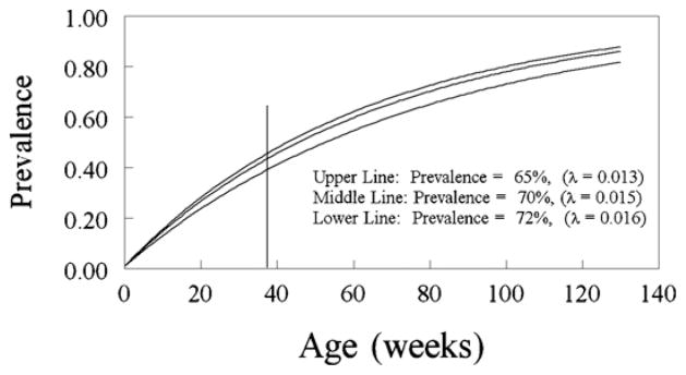
Simulated age-seroprevalence curves for λ = 0.013/week, λ = 0.015/week and λ = 0.016/week based on the model for horizontal transmission. The reported prevalence for each line is the calculated average seroprevalence for mature hosts between 35 and 140 weeks of age based upon the simulation. The model for horizontal transmission was easily able to replicate the highest seroprevalence values observed in the field in the mature age groups (range 64–70%, Van der Leek et al., 1993).

3.2. Sexual transmission, some illustrative scenarios

Fig. 2 illustrates the behavior of the model for sexual transmission as it is allowed to equilibrate given different assumptions about mate guarding and mating systems. In the presence of effective mate guarding (as previously defined), it is impossible to generate the upper part of the range of observed seroprevalence whatever the mating system (Fig. 2a and b). When the mate guarding assumption is abandoned it is possible to generate the observed upper range of seroprevalence but only with high rates of acquisition of new mates (Fig. 2c and d).

Fig. 2.

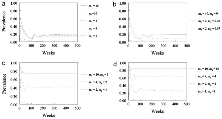
Equilibrium behavior of the model for sexual transmission: the simulated equilibrium prevalence (R₂ + Z₂₁ + Z₂₂ )/(F₂ + M₂₁ + M₂₂ ) in the mature age groups is plotted for each the four scenarios described in Section 2.5 of the main text. Notice that when there is mate guarding, (a) and (b), it is not possible to replicate the highest seroprevalence values observed in the field in the mature age groups (range 64–70%, Van der Leek et al., 1993) even for assumed high rates of acquisition of new mates by the dominant males. As the assumptions about mate guarding and polygyny are relaxed, (c) and (d), it is easier to replicate the high seroprevalence values observed in the field. (a) Scenario 1: polygynous system with perfect mate guarding (m = 1), in which the sub-dominant males never mate (m₈ = 0) and the rate of acquisition of new mates by the dominant males is varied between m₇ = 2 and m₇ = 20; (b) scenario 2: polygynous system with perfect mate guarding (m = 1), in which the sub-dominant males mate with those females not mated with dominant males (i.e. m₇/m₈ = 10/0, 7/0.25, 2/0.67 respectively); (c) scenario 3: polygynous system with no mate guarding, in which sub-dominant males mate with half the number of females as dominant males (m/m₇/m₈ = 6.25/10/5, 2.5/4/2, and 1.25/2/1 respectively); (d) scenario 4: random mating system (no male dominance, no mate guarding) (m/m₇/m₈ = 10/10/10, 4/4/4, 2/2/2 and 1/1/1 respectively).

3.3. Sexual transmission, sensitivity analysis

As noted above, the equilibrium seroprevalence is related to the basic reproduction number, but the basic reproduction number for models of sexual transmission scales in a far from simple way with the overall mean number (M) of new mates acquired per time unit and its variance (V). In general, it can be shown that the basic reproduction number (R₀) is proportional to (M² + V)/M, the precise nature of the relationship being determined by heterogeneities with respect to the risk of infection (Keeling and Rohani, 2008, pp. 57–69). In the particular case of feral swine, for example, the values of M and V vary with the effectiveness of mate guarding and the degree of polygyny (i.e. the assumptions made about the proportion of the male population that is dominant and the average rate of mate acquisition by dominant and subdominant males respectively). We examine this relationship for the particular case of feral swine in Fig. 3, which shows the calculated values of (M² + V)/M for various assumptions about mate guarding and polygyny and the corresponding predicted equilibrium serological prevalence (R₂ + Z₂₁ + Z₂₂)/(F₂ + M₂₁ + M₂₂). Scenarios shown in Fig. 3 can be distinguished according to whether they involve effective mate guarding (the lower trajectories in Fig. 3) or no mate guarding at all (the upper trajectories in Fig. 3). When all females are assumed to have mated and mate guarding is effective, M = 1, R₀ and the corresponding seroprevalence are determined only by the variance of the number of new mates acquired per time unit, which depends upon the average number of new mates acquired by each at-risk group. In polygynous mating systems there are at least three at risk groups: the dominant males, the subdominant males, and the females. When mate guarding is effective, the variance of number of new mates acquired per time unit is greatest when a small number of dominant males can successfully mate with (and guard) a large number of females. In the scenarios examined in this paper, the greatest variance (and hence the largest calculated value for seroprevalence) was obtained when 5% of the males were dominant and each dominant male acquired and successfully guarded 20 new mates per time unit. In this scenario, the subdominant males never acquired new mates and the females acquired one new mate per time unit. The calculated variance was 9.5 (and (M² + V)/M = 10.5; seroprevalence = 20%). A much lower seroprevalence was obtained when 20% of the males were dominant, each dominant male acquired and successfully guarded 4 new mates per time unit, and each subdominant male acquired and successfully guarded 0.25 new mates per time unit. The calculated variance was 1.125 (and (M² + V)/M = 2.125; seroprevalence = 10%) (Fig. 3). Thus, when mate guarding is effective, transmission increases with the degree of polygyny. As the degree of polygyny diminishes, so does transmission (because V gets smaller). Furthermore, under the mate guarding assumption the predicted seroprevalence rapidly tended towards an asymptotic value of about 20% for even the most extreme assumptions regarding the degree of polygyny.

Fig. 3.

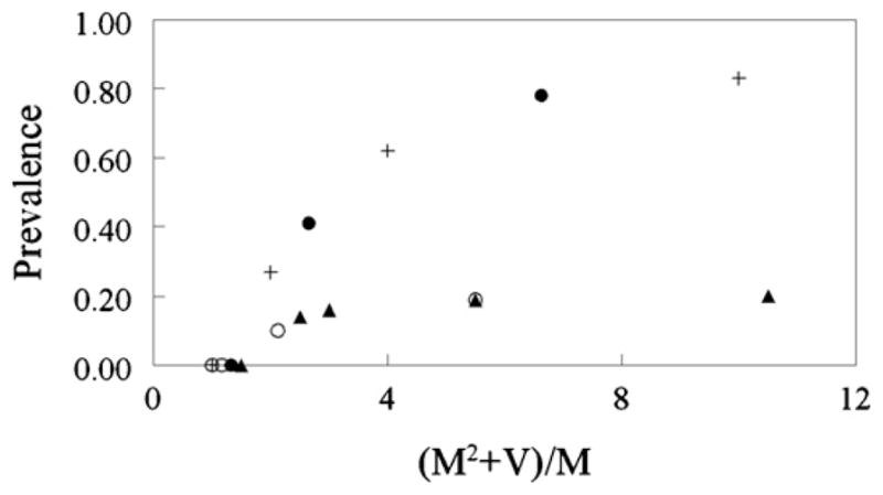
The relationship between the mean (M) and variance (V) of the number of new mates acquired/host/week and the equilibrium seroprevalence of PRV in the mature age groups for each of the four scenarios described in Section 2.5 of the main text. The presence or absence of mate guarding defines the range of possible trajectories irrespective of the other assumptions about the feral mating system. In scenarios 1 and 2, mate guarding is completely effective (lower series of points). In scenarios 3 and 4 there is no mate guarding (upper series of points). Other assumptions as follows: random mating system (+); polygynous system in which sub-dominant males mate with half the number of females as dominant males (●); polygynous system in which the subdominant males never mate (○); polygynous mating system in which subdominant males mate with those females not mated with dominant males (▲).

It becomes easier to generate seroprevalences similar to those observed by Van der Leek et al. (1993) when the mate guarding assumption is abandoned (the upper trajectory in Fig. 3). In these scenarios, it was assumed that the rate at which female pigs acquired new mates was a simple probabilistic consequence of the assumptions made about the proportion of the male population that is dominant and the average rate of mate acquisition by dominant and subdominant males respectively. Thus, when all males had equal access to females and the average number of new mates acquired by any given male was 10 per time unit (for example), the average number of new mates acquired by females was also 10. In such a case, all mature hosts were equally at risk and so the variance, V = 0. Nevertheless, M was large, (M² + V)/M = 10.0 and so the predicted seroprevalence was 83%. When 25% of the males were dominant (i.e. acquired new mates at a rate of 4 per week) and 75% of the males were subdominant (i.e. acquired new mates at rate of 2 per week), the average rate at which females acquired new mates per time unit was given by 4 × 0.25 + 2 × 0.75 = 2.5. In a scenario like this, the three at-risk groups have different risks by reason of the different rate at which they acquire new mates. However, M = 2.5, V = 0.375, (M² + V)/M = 2.65 and so the predicted seroprevalence is much less (41%, see Fig. 3) than for the random mating scenario just considered.

As expected, Fig. 3 also shows that there are values of (M² + V)/M for which the seroprevalence is zero. For this model, when (M² + V)/M < 1.4, the basic reproduction number (R₀) is also less than one and so PRV does not persist in the host population.

3.4. Sexual transmission and sex differences in seroprevalence

If sexual transmission is the only means by which male and female feral swine can be infected with PRV then we would expect the equilibrium seroprevalence in each at-risk group to vary with the rate at which each group acquires new mates. Thus the degree of polygyny and the effectiveness of mate guarding is predicted to profoundly affect the seroprevalence generated for males and females respectively. As expected, in the random mating scenarios (with 1:1 sex ratios), the predicted seroprevalence was the same for both at-risk males and at-risk females. However, in scenarios involving a male dominance hierarchy, the predicted seroprevalence was always different for at-risk males and at-risk females. For example, in a highly polygynous system (10% of the males are dominant and acquire 10 new mates per time unit), 90% of the males are subdominant (never acquire new mates), where mate guarding was effective (females acquire one new mate per time unit) the predicted seroprevalence for at-risk males and at-risk females was 7% and 31% respectively. The reader will remember that Van der Leek et al. (1993) found no significant difference between males and females with respect to seroprevalence at any of the sites in their study.

4. Discussion

The stimulus for the analysis presented here was the report by Romero et al. (2001) that the PRV indigenous to feral swine in the USA is preferentially sexually transmitted. This report is consistent with ecological theory that suggests that sexually transmitted diseases (especially when host sex is confined to a short season each year) will be less severe than other infectious diseases, endemic rather than epidemic and have long infectious periods (Read and Sheldon, 1997). The PRV strains indigenous to feral swine cause little disease (Hahn et al., 1997), epidemics are rarely recorded in the literature, and PRV is a herpes virus that leaves its hosts “latently infected” with the possibility of recrudescence lengthening the effective infectious period (USDA, 2008a). Romero et al. (2001) were careful to state that PRV in feral swine was preferentially sexually transmitted thus leaving open the possibility for other transmission modalities. Nevertheless, they did argue that “based on these results, we feel that as long as feral swine do not come into direct contact with domestic swine, PRV-infected feral swine probably pose only a limited risk to the success of the National Pseudorabies Eradication Program”. If sexual transmission is indeed the predominant route of transmission of PRV in feral swine, then models incorporating that mechanism alone should have little difficulty in replicating the range of seroprevalence values observed in the field. The analysis presented above shows that this is true only for certain (fairly extreme) assumptions about feral swine mating systems in the USA.

The pseudorabies virus is frequently used as a laboratory model for herpes viruses in general and there are clear indications that genetic variation can influence both pathogenicity and transmission (Glorieux et al., 2009; Kramer et al., 2011), which might have provided an explanation for the supposed differences in transmission of the virus with domestic and feral swine. However, a recent analysis by Hahn et al. (2010) finds that, although most PRV from feral swine can be distinguished from virus circulating in domestic pigs during the national epizootic, several feral swine isolates of PRV from south central states are closely related to strains from domestic pigs. Furthermore, the same workers stated that “Many people have misinterpreted and focused on the notion that transmission among wild pigs is exclusively venereal. This was never meant in the original demonstration of feral pig venereal transmission, but too many thought this mode as the only mechanism operating in the wild,” and conclude, “Clearly the virus in feral swine has multiple mechanisms of transmission to insure persistent infection and the threat of re-emergence in domestic swine continues” (Hahn et al., 2010). This is essentially the same conclusion that this paper has drawn from an analysis of competing models for transmission.

In the simplest form of the first model, horizontal (non-sexual) density dependent transmission is the only transmission modality. In the second model, the only transmission modality is sexual transmission between mature males and females. Sexual transmission depends upon the rate of acquisition of new mates whereas non-sexual horizontal transmission depends upon some index of host abundance (in this case population density). It was straightforward to generate the range of seroprevalence recorded for feral swine in the USA when non-sexual horizontal transmission was the only transmission modality and when sexual transmission involved a random mating system. It was more difficult to generate the upper part of the range of observed seroprevalence in the sexual transmission model when there was some degree of polygyny, and it was impossible to generate all but the very lowest range of observed values when mate guarding was sufficiently effective to prevent females mating with more than one male for the duration of the infectious period (about one week). In addition, incorporating polygyny and mate guarding into the model always resulted in a sex difference in the simulated seroprevalence; sex differences in seroprevalence are not a typical feature of the field data. In short, the observed range of seroprevalence of PRV in mature feral swine in the USA is not consistent with a preferential sexual transmission if there is mate guarding and the mate guarding is sufficiently effective to prevent females mating with more than one male for the duration of the infectious period (about one week). Indeed, mate guarding will always reduce seroprevalence.

There is no consensus view about the mating system of feral pigs in the USA and it is relevant that our notions about what happens in the USA are garnered from studies based in Australia and Europe as well as in the USA. The older literature assumed that the mating system in wild boars was highly polygynous (Beuerle, 1975; Poteaux et al., 2009; Boitani et al., 1994) but more recent studies have led several groups to suggest instead that there is only a “moderate” level of polygyny (Hampton et al., 2004; Spencer et al., 2005; Poteaux et al., 2009). Mate guarding has several times been invoked as an explanation for the rarity of multiple paternity of single litters (Delgado et al., 2008; Poteaux et al., 2009). The fact that there is not usually any sex difference in the seroprevalence observed in mature feral swine in the USA is not consistent with a polygynous system of mating (especially if there is mate guarding as well) but is difficult to reconcile with the older literature on the social structure and mating systems of feral swine. On the other hand, the random (or almost random) mating systems that some researchers have used to explain genetic data from Australia (Hampton et al., 2004) could easily explain the discrepancy and generate the observed seroprevalence for quite modest assumptions about the rate of acquisition of new mates – but so too could a model which combined sexual and non-sexual horizontal transmission.

Until we better understand the nature of the feral swine mating system the USA and have data on the rate of acquisition of new mates, it seems prudent to assume that PRV in feral swine is transmitted both sexually and non-sexually. Measurements on the rate of acquisition of new mates are particularly important. The spread of a sexually transmitted disease does not depend upon the number of times hosts mate, but rather upon the number of times they mate with a new mate. Of particular importance is the average number of times a typical host mates with a new mate during a period of time equivalent to the duration of infectiousness. If, on average, a host mates with a new mate only once during this period, that is not sufficient to acquire and transmit the infection. For PRV, this would require that a typical host would have to acquire an average of, at least, two new mates every week. In order to generate the seroprevalence observed in the field, some implementations of the model for sexual transmission described here required a weekly rate of acquisition of new mates many times that.

Appendix A. Supplementary data

Supplementary data associated with this article can be found, in the online version, at doi:10.1016/j.prevetmed.2011.09.010.

References

- Anderson RM, May RM. Infectious Diseases of Humans: Dynamics and Control. Oxford University Press; Oxford: 1991. [Google Scholar]
- Begon M, Bennett M, Bowers RG, French NP, Hazel SM, Turner J. A clarification of transmission terms in host-microparasite models: numbers, densities and areas. Epidemiol Infect. 2002;129:147–153. doi: 10.1017/s0950268802007148. [DOI] [PMC free article] [PubMed] [Google Scholar]
- Beuerle W. Field observations of aggressive sexual behaviour in European wild hog (Sus scrofa L.) Z Tierpsych. 1975;39:211–258. [PubMed] [Google Scholar]
- Bieber C, Ruf T. Population dynamics in wild boar (Sus scrofa): ecology, elasticity of growth rate and implications for the management of pulsed resource consumers. J Appl Ecol. 2005;42:1203–1213. [Google Scholar]
- Boitani L, Mattei L, Nonis D, Corsi F. Spatial and activity patterns of wild boars in Tuscany, Italy. J Mammal. 1994;75:600–612. [Google Scholar]
- Bouma A, de Jong MCM, Kimman TG. Transmission of pseudorabies within pig populations is independent of the size of the population. Prev Vet Med. 1995;23:163–172. [Google Scholar]
- Caley P, Hunt NT, Melville L. Age-specific prevalence of porcine parvovirus antibody in feral pigs from a site in the Northern Territory. Aust Vet J. 1995;72:36–37. doi: 10.1111/j.1751-0813.1995.tb03476.x. [DOI] [PubMed] [Google Scholar]
- Campbell TA, DeYoung RW, Wehland EM, Grassman LI, Long DB, Delgado-Acevedo J. Feral swine exposure to selected viral and bacterial pathogens in southern Texas. J Swine Health Prod. 2008;16:312–315. [Google Scholar]
- Corn JL, Stallknecht DE, Mechlin NM, Luttrell MP, Fischer JR. Persistence of pseudorabies virus in feral swine populations. J Wildl Dis. 2004;40:307–310. doi: 10.7589/0090-3558-40.2.307. [DOI] [PubMed] [Google Scholar]
- Corn JL, Cumbee JC, Barfoot R, Erickson GA. Pathogen exposure in feral swine populations geographically associated with high densities of transitional swine premises and commercial swine production. J Wildl Dis. 2009;45:713–721. doi: 10.7589/0090-3558-45.3.713. [DOI] [PubMed] [Google Scholar]
- Davies EB, Beran GW. Spontaneous shedding of pseudorabies from a clinically recovered post parturient sow. JAVMA. 1980;176:1345–1347. [PubMed] [Google Scholar]
- Davies EB, Beran GW. Influence of environmental factors upon the survival of Aujeszky’s disease virus. Res Vet Sci. 1981;31:32–36. [PubMed] [Google Scholar]
- Delgado R, Fernandez-Llario P, Azevedoc M, Beja-Pereirac A, Santos P. Paternity assessment in free-ranging wild boar (Sus scrofa) –are littermates full-sibs? Mamm Biol. 2008;73:169–176. [Google Scholar]
- Dewsbury DA. A test of the role of copulatory plugs in sperm competition in deer mice (Peromyscus maniculatus) J Mammal. 1988;69:854–857. [Google Scholar]
- Donaldson AI, Wardley RC, Martin S, Harkness JW. Influence of vaccination of Aujesky’s disease virus and disease transmission. Vet Rec. 1984;115:121–124. doi: 10.1136/vr.115.6.121. [DOI] [PubMed] [Google Scholar]
- Gardner IA, Willeberg P, Mousing J. Empirical and theoretical evidence for herd size as a risk factor for swine diseases. Anim Health Res Rev. 2002;3:43–55. doi: 10.1079/ahrr200239. [DOI] [PubMed] [Google Scholar]
- Geisser H, Reyer HU. The influence of food and temperature on population density of wild boar Sus scrofa in the Thurgau (Switzerland) J Zool Lond. 2005;267:89–96. [Google Scholar]
- Glorieux S, Favoreel HW, Meesen G, de Vos W, Van den Broeck W, Nauwynck HJ. Different replication characteristics of historical pseudorabies virus strains in porcine respiratory nasal mucosa explants. Vet Microbiol. 2009;136:341–346. doi: 10.1016/j.vetmic.2008.11.005. [DOI] [PubMed] [Google Scholar]
- Greenwell R. The Ricker salmon model. UMAP J. 1984;5:337–359. [Google Scholar]
- Gresham CS, Gresham CA, Duffy MJ, Faulkner CT, Patton S. Increased prevalence of Brucella suis and pseudorabies virus antibodies in adults of an isolated feral swine population in coastal South Carolina. J Wildl Dis. 2002;38:653–656. doi: 10.7589/0090-3558-38.3.653. [DOI] [PubMed] [Google Scholar]
- Groot Bruinderink GWTA, Hazebroek E. Modelling carrying capacity for wild boar, Sus scofa scrofa, in a forest/heathland ecosystem. Wildl Biol. 1995;1:81–87. [Google Scholar]
- Gustafson DP. Pseudorabies. In: Leman AD, Straw B, Glock RD, et al., editors. Diseases of Swin. 6. Iowa State University Press; Ames, Iowa: 1986. pp. 274–289. [Google Scholar]
- Hahn EC, Page GR, Hahn PS, Gillis KD, Romero C, Annelli JA, Gibbs EPJ. Mechanisms of transmission of Aujesky’s disease virus originating from feral swine in the USA. Vet Microbiol. 1997;55:123–130. doi: 10.1016/s0378-1135(96)01309-0. [DOI] [PubMed] [Google Scholar]
- Hahn EC, Fadl-Alla B, Lichtensteiger CA. Variation of Aujeszky’s disease viruses in wild swine in USA. Vet Microbiol. 2010;143:45–51. doi: 10.1016/j.vetmic.2010.02.013. [DOI] [PubMed] [Google Scholar]
- Hampton J, Pluske JR, Spencer PBS. A preliminary genetic study of the social biology of feral pigs in south-western Australia and the implications for management. Wildl Res. 2004;31:375–381. [Google Scholar]
- Hebeisen C, Fattebert J, Baubet E, Fischer C. Estimating wild boar (Sus scrofa) abundance and density using capture–resights in Canton of Geneva, Switzerland. Eur J Wildl Res. 2008;54:391–401. [Google Scholar]
- Hone J. Predator–prey theory and feral pig control, with emphasis on evaluation of shooting from a helicopter. Aust Wildl Res. 1990;17:123–130. [Google Scholar]
- Hynes EF, Rudd CD, Temple-Smith PD, Sofronidis G, Paris D, Shaw G, Renfree MB. Mating sequence, dominance and paternity success in captive male tammar wallabies. Reproduction. 2005;130:123–130. doi: 10.1530/rep.1.00624. [DOI] [PubMed] [Google Scholar]
- Jia Z, Duan E, Jiang Z, Wang Z. Copulatory plugs in masked palm civets: prevention of semen leakage, sperm storage, or chastity enhancement? J Mammal. 2002;83:1035–1038. [Google Scholar]
- Kaminski G, Brandt S, Baubet E, Baudoin C. Life-history patterns in female wild boars (Sus scrofa): mother–daughter postweaning associations. Can J Zool. 2005;83:474–480. [Google Scholar]
- Keeling MJ, Rohani P. Modeling Infectious Diseases in Humans and Animals. Princeton University Press; Princeton and Oxford: 2008. [Google Scholar]
- Kramer T, Greco TM, Enquist LW, Cristea IM. Proteomic characterization of pseudorabies virus extracellular virions. J Virol. 2011;85:6427–6441. doi: 10.1128/JVI.02253-10. [DOI] [PMC free article] [PubMed] [Google Scholar]
- Krebs CL. Ecology: The Experimental Analysis of Distribution and Abundance. Harper and Row; New York: 1972. [Google Scholar]
- Lambert JD, Lambert D. Numerical Methods for Ordinary Differential Systems: The Initial Value Problem. Chapter 5 Wiley; New York: 1991. [Google Scholar]
- Lari A, Lorenzi D, Nigrelli D, Brocchi E, Faccini S, Poli A. Pseudorabies virus in European wild boar from Central Italy. J Wildl Dis. 2006;42:319–324. doi: 10.7589/0090-3558-42.2.319. [DOI] [PubMed] [Google Scholar]
- Lutz W, Langhans DJ, Schmitz D, Müller T. A long-term survey of pseudorabies virus infections in European wild boar of western Germany. Z Jagdwiss. 2003;49:130–140. [Google Scholar]
- Massolo A, Mazzoni della Stella R. Population structure variations of wild boar Sus scrofa in central Italy. Ital J Zool. 2006;73:137–144. [Google Scholar]
- Maes L, Pensaert M. Persistence of Aueszky’s virus on fattening and breeding premises for pigs after an outbreak of the disease. Tijdschr Diergeneeskd. 1984;109:439–445. [PubMed] [Google Scholar]
- McFerran JB, Dow C. The effect of colostrum derived antibody on mortality and virus excretion following experimental infection of piglets with Aujeszky’s disease virus. Res Vet Sci. 1973;15:208–214. [PubMed] [Google Scholar]
- Merdan H, Duman O, Akin O, Celik C. Allee effects on population dynamics in continuous (overlapping) case. Chaos Soliton Fract. 2009;39:1994–2001. [Google Scholar]
- Miller AR. A test for life tables for theoretical gerontology. J Gerontol. 1988;43:B43–B49. doi: 10.1093/geronj/43.2.b43. [DOI] [PubMed] [Google Scholar]
- Mockeliuniene V, Salomaskas A, Mockeliunas R, Petkevicius S. Prevalence and epidemiological features of bovine viral diarrhoea virus infection in Lithuania. Vet Microbiol. 2004;99:51–57. doi: 10.1016/j.vetmic.2003.11.008. [DOI] [PubMed] [Google Scholar]
- Parga JA. Copulatory plug displacement evidences sperm competition in Lemur catta. Int J Primatol. 2003;24:889–899. [Google Scholar]
- Pech RB, Hone J. A model of the dynamics and control of an outbreak of foot and mouth disease in feral pigs in Australia. J Appl Ecol. 1988;25:63–77. [Google Scholar]
- Pirtle EC, Sacks JM, Nettles VF, Rollor EA. Prevalence and transmission of pseudorabies virus in an isolated population of feral swine. J Wildl Dis. 1989;25:605–607. doi: 10.7589/0090-3558-25.4.605. [DOI] [PubMed] [Google Scholar]
- Pohlmeyer K, Sodeikat G. Population dynamics and habitat use of wild boar in Lower Saxony. Workshop on Classical Swine Fever; October 6th–9th, 2003; Hannover. 2003. pp. 1–4. (AGRO307/7730) [Google Scholar]
- Poteaux C, Baubet E, Kaminski G, Brandt S, Dobson FS, Baudoin C. Sociogenetic structure and mating system of a wild boar population. J Zool. 2009;278:116–125. [Google Scholar]
- Read AF, Sheldon BC. Comparative biology and disease ecology. TREE. 1997;12:43–44. doi: 10.1016/s0169-5347(96)30062-1. [DOI] [PubMed] [Google Scholar]
- Rosell C, Navàs F, Romero S, de Dalmases I. Activity patterns and social organization of wild boar (Sus scrofa L.) in a wetland environment: preliminary data on the effects of shooting individuals. Galemys. 2004;16:157–166. (Special issue) [Google Scholar]
- Romero CH, Meade PN, Shultz JE, Chung HY, Gibbs EP, Hahn EC, Lollis G. Venereal transmission of pseudorabies viruses indigenous to feral swine. J Wildl Dis. 2001;37:289–296. doi: 10.7589/0090-3558-37.2.289. [DOI] [PubMed] [Google Scholar]
- Rossi S, Fromont E, Pontier D, Cruciere C, Hars J, Barrat J, Pacholek X, Artois M. Incidence and persistence of classical swine fever in free-ranging wild boar (Sus scrofa) Epidemiol Infect. 2005;133:559–568. doi: 10.1017/s0950268804003553. [DOI] [PMC free article] [PubMed] [Google Scholar]
- Ruiz-Fons F, Vidal D, Hofle U, Vicente J, Gortazar C. Aujeszky’s disease virus infection patterns in European wild boar. Vet Microbiol. 2007;120:241–250. doi: 10.1016/j.vetmic.2006.11.003. [DOI] [PubMed] [Google Scholar]
- Sharif M, Daryani A, Nasrolahei M, Ziapour SP. Prevalence of Toxoplasma gondii antibodies in stray cats in Sari, northern Iran. Trop Anim Health Prod. 2009;41:183–187. doi: 10.1007/s11250-008-9173-y. [DOI] [PubMed] [Google Scholar]
- Schoenbaum MA, Beran GW, Murphy DP. Pseudorabies virus latency and reactivation in vaccinated swine. Am J Vet Res. 1990;51:334–338. [PubMed] [Google Scholar]
- Smith G, Grenfell BT. The population biology of pseudorabies in swine. Am J Vet Res. 1990;51:148–155. [PubMed] [Google Scholar]
- Spencer P, Lapidge S, Hampton J, Pluske J. The sociogenetic structure of a controlled feral pig population. Wildl Res. 2005;32:297–304. [Google Scholar]
- Sweitzer RA, Van Vuren D, Gardner IA, Boyce WM, Waithman JD. Estimating sizes of wild pig populations in the north and central coast regions of California. J Wildl Manage. 2000;64:531–543. [Google Scholar]
- USDA. Pseudorabies (Aujeszky’s Disease) and Its Eradication a Review of the US Experience. United States Department of Agriculture, Animal and Plant Health Inspection Service; 2008a. Technical Bulletin No. 1923. [Google Scholar]
- USDA. National Pseudorabies Surveillance Plan: Final Draft, Version 1.01. United States Department of Agriculture, Animal and Plant Health Inspection Service, Veterinary Services Centers for Epidemiology and Animal Health, National Surveillance Unit; Fort Collins, CO: 2008b. Apr 16, [Google Scholar]
- Van der Leek ML, Becker HN, Pirtle EC, Humphrey P, Adams CL, All BP, Erickson GA, Belden RC, Frankenberger WB, Gibbs EPJ. Prevalence of pseudorabies (Aujeszky’s disease) virus antibodies in feral swine in Florida. J Wildl Dis. 1993;25:605–607. doi: 10.7589/0090-3558-29.3.403. [DOI] [PubMed] [Google Scholar]
- Vicente J, Ruiz-Fons F, Vidal D, Höfle U, Acevedo P, Villanúa D, Fernández-de-Mera IG, Martín MP, Gortázar C. Serosurvey of Aujeszky’s disease virus infection in European wild boar in Spain. Vet Rec. 2005;156:408–412. doi: 10.1136/vr.156.13.408. [DOI] [PubMed] [Google Scholar]
- West BC, Cooper AL, Armstrong JB. Managing wild pigs: a technical guide. Human–Wildlife Interactions Monograph. 2009;1:1–55. [Google Scholar]
- Wyckoff AC, Henke SE, Campbell TA, Hewitt DG, VerCauteren KC. Feral swine contact with domestic swine: a serologic survey and assessment of potential for disease transmission. J Wildl Dis. 2009;45:422–429. doi: 10.7589/0090-3558-45.2.422. [DOI] [PubMed] [Google Scholar]
Associated Data
This section collects any data citations, data availability statements, or supplementary materials included in this article.