Relation between free energy landscapes of proteins and dynamics

Abstract

By examining the molecular dynamics (MD) of protein folding trajectories, generated with the coarse-grained UNRES force field, for the B-domain of staphylococcal protein A and the triple β-strand WW domain from the Formin binding protein 28 (FBP), by principal component analysis (PCA), it is demonstrated how different free energy landscapes (FELs) and folding pathways of trajectories can be, even though they appear to be very similar by visual inspection of the time-dependence of the root-mean-square deviation (rmsd). Approaches to determine the minimal dimensionality of FELs for a correct description of protein folding dynamics are discussed. The correlation between the amplitude of the fluctuations of proteins and the dimensionality of the FELs is shown. The advantage of internal coordinate PCA over Cartesian PCA for small proteins is also illustrated.

1. Introduction

Protein folding is a rapid and complex process that is difficult to characterize because folding does not refer to the progressive pathway of a single conformation. Instead, it pertains to interconversions among ensembles of conformations in a back-and-forth progression from the non-native to the native state. In addition, the non-native and native states themselves may consist of a large ensemble of conformations, interconverting at a rapid rate, and characterized by basins with many minima in each state. A folding pathway is not always defined in terms of a two-state model consisting of the non-native and the native state separated by the energetically unfavorable transition state. Proteins can fold through intermediate states^1,2 or undergo one-state downhill folding.^1,3 Therefore, finding the coordinates along which the intrinsic folding pathways of biological molecules (containing thousands of degrees of freedom) can be identified still remains a challenge.

A study of free-energy landscapes (FELs) provides an understanding of how proteins fold and function.^4-6 It should be noted that the FELs determined from canonical MD simulations at temperatures significantly lower than the folding-transition temperature are usually non-equilibrium landscapes because canonical simulations take very long to equilibrate. Generalized-ensemble algorithms,⁷ in which walks in temperature or energy space are performed, converge much faster than canonical sampling and should be used to obtain equilibrium FEL’s. On the other hand, the non-equilibrium FEL’s resulting from canonical simulations are also valuable, because they provide condensed information about the frequency of visiting particular regions of conformational space during the simulated folding. It must be borne in mind, though, that these FEL’s are dependent on simulation setup such as trajectory length, the number of trajectories run at a given temperature, and even the starting conformation(s). In this paper, we discuss the FEL’s calculated from canonical trajectories which, as remarked above, are generally not equilibrated. However, because we ran our calculations close to the folding-transition temperatures for both proteins studied, which lowers the free energy barriers between conformational states, the FEL’s should be close to equilibrium FEL’s. Molecular dynamics (MD) simulations based on atomic⁸ and coarse-grained⁹ models provide the atomic- and coarse-grained-level pictures, respectively, of protein motion and the connection to the underlying FEL. The commonly-used reaction coordinates [radius of gyration (R_g), root-mean-square deviation (rmsd) with respect to the native state, etc.] are arbitrary ones, and do not necessarily capture the features of protein energy landscapes. In order to overcome these problems, many different methods have been developed for the past two decades, for example, the approaches based on transition networks,^10,11 an unprojected representation of FEL. Another frequently used method for defining reaction coordinates is a covariance-matrix-based mathematical technique, called principal component analysis (PCA),¹² which typically captures most of the total displacement from the average protein structure with the first few principal components (PCs) during a simulation.

Although PCA reduces the dimensionality of a complex system drastically, the low-dimensional [one-dimensional (1-D) or two-dimensional (2-D)] representation of an FEL does not always provide a correct picture, and may lead to serious artifacts.^13,14 How complete are 1-D and 2-D FELs? How correct are the protein-folding kinetics and diffusive behavior described by 1-D and 2-D FELs? These questions were addressed in a preliminary way in our recent study.¹⁵ An analysis of the different-dimensional FELs for a folding/unfolding trajectory of the B-domain of staphylococcal protein A (1BDD), a 46-residue three-α-helical protein,¹⁶ showed that the low-dimensional FELs are not always sufficient for the description of folding/unfolding processes.¹⁵

In the present work, we continue our study of the relation between FELs and a correct description of folding dynamics. For this purpose, we ran 110 trajectories of canonical MD simulations with the coarse-grained united-residue (UNRES) force field^17-22 at different temperatures for both 1BDD and the 37-residue triple-β-stranded WW domain from the Formin binding protein 28 (FBP) (1E0L),²³ and investigated one folding trajectory in detail for each protein. Based on their rmsd as a function of time, the behavior of each protein is simple and similar to each other [panel (b) in Figures 1 and 2]. In particular, both proteins fold directly from the unfolded state to the native-like conformation and remain there for the rest of the simulations.

Figure 1.

(a) Experimental NMR structure of B-domain of staphylococcal protein A, (b) rmsd from the native structure as a function of time, (c) free energy profile (FEP) (in kcal/mol) plotted as a function of rmsd, and (d) FEL (in kcal/mol) plotted as a function of rmsd and radius of gyration for 1BDD.

Figure 2.

Same as in Figure 1 but for 1E0L.

In our recent preliminary study,¹⁵ we investigated a more complex trajectory of 1BDD in which frequent transitions between the native and unfolded structures occurred; consequently, the question arises as to whether the complexity of the pathway could be the reason that a one- or two-dimensional FEL sometimes fails to describe the behavior of the system. We demonstrate how to determine the lowest-dimensional FEL for each trajectory, which can describe the folding dynamics correctly, and show the correlation between the percentage of the fluctuations captured by the PCs and the dimensionality of the FEL necessary for a correct description of folding/unfolding processes. We also demonstrate that the FELs of coarse-grained folding trajectories obtained from internal coordinate PCA^24-27 are more rugged than those constructed by traditional Cartesian PCA.

It should be noted that both 1BDD and 1E0L proteins have been the subject of extensive theoretical^8,9,15,27-41 and experimental^2,42-46 studies because of their small size, fast-folding kinetics and biological importance. As a related phenomenon, the formation of intermolecular β-sheets is thought to be a crucial event in the initiation and propagation of amyloid diseases such as Alzheimer’s disease⁴⁷ and spongiform encephalopathy.⁴⁸

This paper is organized as follows. The UNRES force-field and PCA method are reviewed in Section 2. The results are discussed in Section 3. A summary and conclusions are presented in Section 4.

2. Methods

UNRES model and simulation details

The UNRES model of polypeptide chains^{18,19,22,49,50} is illustrated in Figure 3. A polypeptide chain is represented as a sequence of α-carbon (C^α) atoms linked by virtual C^α…C^α bonds with united peptide groups halfway between the neighboring C^α’s, and united side chains, whose sizes depend on the nature of the amino acid residues, attached to the respective C^α’s by virtual C^α…SC bonds. The effective energy is expressed by Eq. 1.²²

$$\begin{array}{cc}\hfill U=& w_{\mathit{SC}}\sum _{i<j}{U}_{{\mathit{SC}}_i{\mathit{SC}}_j}+w_{{\mathit{SC}}_p}\sum _{i\ne j}{U}_{{\mathit{SC}}_i{p}_j}+w_{pp}{f}_2\left(T\right)\sum _{i<j-1}{U}_{p_i{p}_j}+w_{\text{tor}}{f}_2\left(T\right)\sum _i{U}_{\text{tor}}\left({\gamma }_i\right)\hfill \\ \hfill & +w_{\text{tord}}{f}_3\left(T\right)\sum _i{U}_{\text{tord}}({\gamma }_i,{\gamma }_{i+1})+w_b\sum _i{U}_b\left({\theta }_i\right)+w_{\mathit{rot}}\sum _i{U}_{\mathit{rot}}({\alpha }_{{\mathit{SC}}_i},{\beta }_{{\mathit{SC}}_i},{\theta }_i)\hfill \\ \hfill & +w_{\text{bond}}\sum _i{U}_{\text{bond}}\left(d_i\right)+\sum _{m=3}^6{w}_{\mathit{corr}}^{\left(m\right)}{f}_m\left(T\right)U_{\mathit{corr}}^{\left(m\right)}+w_{\mathit{SS}}\sum _i{U}_{\mathit{SS};i}\hfill \end{array}$$ (1)

with²²

$$f_m\left(T\right)=\frac{\ln (e+e^{-1})}{\ln \left\{\exp \left[{\left(\frac{T}{T_0}\right)}^{m-1}\right]+\exp \left[-{\left(\frac{T}{T_0}\right)}^{m-1}\right]\right\}};T_0=300K$$ (2)

where the successive terms represent side chain-side chain, side chain-peptide, peptide-peptide, torsional, double-torsional, bond-angle bending, side-chain local (dependent on the angles α and β of Fig. 3), distortion of virtual bonds, multi-body (correlation) interactions, and formation of disulfide bonds, respectively. The w’s are the relative weights of each term. The correlation terms arise from a cumulant expansion^50,51 of the restricted free energy function of the simplified chain obtained from the all-atom energy surface by integrating out the secondary degrees of freedom. The temperature-dependent factors of Eq. 2, introduced in our recent work²² and discussed further in reference 52, reflect the fact that the UNRES effective energy is an approximate cumulant expansion of the restricted free energy. The virtual-bond vectors are the variables used in molecular dynamics.

Figure 3.

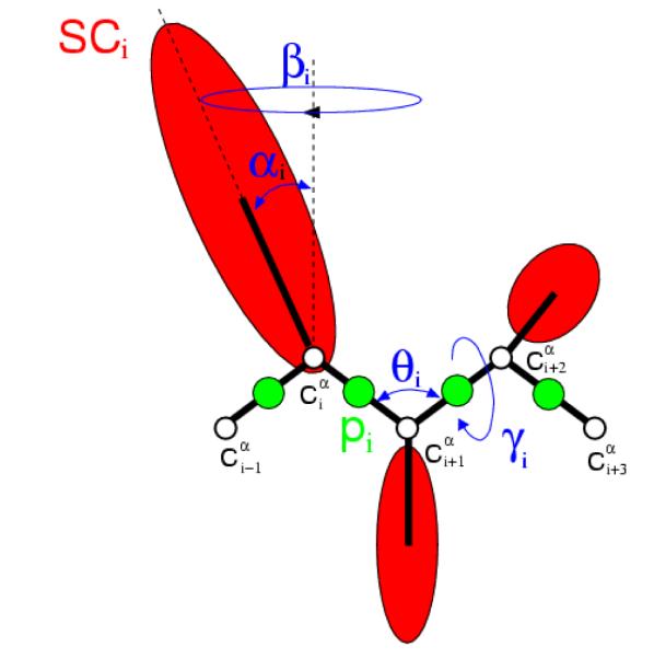
The UNRES model of polypeptide chains. The interaction sites are red side-chain centroids of different sizes (SC) and the peptide-bond centers (p) are indicated by green circles, whereas the α-carbon atoms (small empty circles) are introduced only to assist in defining the geometry. The virtual C^α⋯C^α bonds have a fixed length of 3.8 $\acute{\mathrm{Å}}$, corresponding to a trans peptide group; the virtual-bond (θ) and virtual-dihedral (γ) angles are variable. Each side chain is attached to the corresponding α-carbon with a fixed “bond length”, b_SCi, variable “bond angle”, α_i, formed by SC_i and the bisector of the angle defined by $C_{i-1}^{\alpha }$,$C_i^{\alpha }$, and $C_{i+1}^{\alpha }$, with a variable “dihedral angle”, β_i, of counter-clockwise rotation about the $C_{i-1}^{\alpha }$, $C_i^{\alpha }$, $C_{i+1}^{\alpha }$ frame.

For 1BDD, we ran canonical UNRES molecular dynamics trajectories³⁸ at 11 temperatures at 5° intervals between 290 and 340K, with 10 trajectories at each temperature (for a total of 110 trajectories). The force field parameterized on 1GAB²² was used. For 1E0L, we carried out canonical MD runs at the following 11 temperatures: 280, 290, 300, 310, 320, 330, 335, 340, 345, 350, and 360 K, with 10 trajectories at each temperature (for a total of 110 trajectories), with the force field parameterized on 1E0L and 1ENH.⁵³ The Berendsen thermostat⁵⁴ was used to maintain constant temperature. The trajectories selected for detailed analysis corresponded to near folding-transition temperature: T = 310 K for 1BDD (T_f = 320 K)²² and 330K for 1E0L (T_f = 339 K),⁵³ since these are the most favorable temperature regions for folding both proteins. The time step in molecular dynamics simulations was δt = 0.1 mtu (1 mtu = 48.9 fs is the “natural” time unit of molecular dynamics⁵⁵) and the coupling parameter of the Berendsen thermostat was τ = 1 mtu. For each trajectory, a total of 35,000,000 steps (about 0.175 μs of MD time) were run for 1BDD and 120,000,000 steps (about 0.6 μs of MD time) were run for 1E0L.

Principal component analysis

The PCA method¹² is based on the covariance matrix with elements C_ij for coordinates i and j

$$C_{\mathit{ij}}=\langle (x_i-\langle x_i\rangle )(x_j-\langle x_j\rangle )\rangle$$ (3)

where x₁,…, x_3N are the mass-weighted Cartesian coordinates of an N-particle system and ⟨ ⟩ is the average over all instantaneous structures sampled during the simulations. The symmetric 3N × 3N matrix C can be diagonalized with an orthonormal transformation matrix R:

$${\mathbf{R}}^{\mathbf{T}}\mathbf{CR}=\text{diag}({\lambda }_1,{\lambda }_2,\dots ,{\lambda }_{3\mathrm{N}}),$$ (4)

where λ₁ ≥ λ₂ ≥ … ≥ λ_3N are the eigenvalues, and R^T is the transpose of R. The columns of R are the eigenvectors, or the principal modes; the trajectory can be projected onto the eigenvectors to give the principal components q_i(t), i = 1, …, 3N:

$$\mathbf{q}={\mathbf{R}}^{\mathbf{T}}\left(\mathbf{X}\right(\mathrm{t})>\mathbf{x}>)$$ (5)

The eigenvalue λ_i is the mean-square fluctuation in the direction of the principal mode. The first few PCs typically describe collective, global motions of the system, with the first PC containing the largest mean-square fluctuation.

Since we study the coarse-grained MD trajectories, in PCA we replaced the Cartesian coordinates by UNRES backbone coordinates (θ_i, γ_j),

$$\begin{array}{cc}\hfill & x_i=\cos \left({\theta }_i\right)x_{i+1}=\sin \left({\theta }_i\right),\hfill \\ \hfill & x_j=\cos \left({\gamma }_j\right),x_{j+1}=\sin \left({\gamma }_j\right).\hfill \end{array}$$ (6)

where i = 1, … , N-2 and j = 1, …, N -3, are the numbers of θ and γ angles, respectively, N being the number of amino-acid residues in the chain. As shown by Mu et al.²⁴ and Altis et al.,²⁶ such a transformation from the space of backbone angles to a linear metric coordinate space enables us to avoid potential problems due to the periodicity of the angles.

3. Results and discussion

3.1. Determination of least-dimension, correctly-describing folding dynamics FEL

Based on the results [rmsd vs time, free energy profile (FEP) as a function of rmsd, and FEL as a function of rmsd and R_g)] shown in Figures 1 and 2, both proteins seem to fold following a two-state model with low-energy non-native and native states separated by a single energy barrier. The one-dimensional FELs, i.e., FEPs, suggest a simple picture containing the “unfolded” (high rmsd) and “folded” (low rmsd) states. The 2-D FELs reveal a more complex picture because the high-rmsd mimina correspond to low radii of gyration (R_g). Consequently, the high-rmsd states should be regarded as misfolded and not unfolded states, indicating that both systems can get trapped in metastable conformations during folding. The loose unfolded conformations are present only during a few thousand initial steps of the simulations and then both proteins collapse rapidly to either roughly folded or misfolded conformations. The complexity of the FELs obtained from simulations is consistent with the experimentally observed multiple-exponential kinetics of both proteins.^2,56

While the folded state is unique, the misfolded one does not have to be and, consequently, the description provided by the 2-D rmsd-R_g FEL plot might be oversimplified and misleading. We, therefore, employed a PCA to study the folding dynamics of 1BDD and 1E0L, particularly internal-coordinate PCA, because FELs of small systems constructed by traditional Cartesian PCA may contain artifacts arising from strong mixing of overall and internal motion.^24-26 This issue will be addressed in sub-section 3.3.

As mentioned above, the first few PCs can capture more than half of the total fluctuation in the system; however, it is important to specify the criterion for selecting the PCs along which an FEL can be constructed. Based on the fact that the multiply-hierarchical PCs are a main contributor to the total fluctuations, and the subspace formed by multiply-hierarchical PCs contains the most important molecular conformations,⁵⁷ Hegger et al.⁵⁸ defined the dimension of the free energy landscape by the fewest number of multiply-hierarchical PCs. Figures 4 and 5 illustrate the probability distribution functions P(q) of the first five PCs (a); the FEP, μ(q₁) = −k_BT ln P(q₁) , along the first PC (b); the 2-D FEL along the first two PCs, μ(q₁,q₂) = −k_BT ln P(q₁,q₂) (c); and the 3-D FEL along the first three PCs, μ(q₁,q₂,q₃) = −k_BT ln P(q₁,q₂,q₃) (d), with T and k_B being the absolute temperature and the Boltzmann constant, respectively, for 1BDD and 1E0L, respectively.

Figure 4.

The probability distribution function for the first five internal coordinate PCs of 1BDD (a), 1-D (b), 2-D (c), and 3-D (d) FELs (in kcal/mol) along internal coordinate PCs.

Figure 5.

The same as in Figure 4 but for 1E0L.

As in our previous study¹⁵ carried out with a seemingly more complex folding pathway of 1BDD, the shapes of the P(q)’s [panel (a) in Figure 4] suggest that the first four PCs of 1BDD clearly belong to the multiply-hierarchical category which means that, for a correct representation of the folding dynamics of 1BDD, we need a 4-D FEL. This observation is further corroborated by the 1-D, 2-D, and 3-D FELs depicted in panels (b, c, d) of Figure 4, which show how much information is hidden in low-dimensional FELs. Although five minima are indicated in the 1-D FEP [panel (b) Figure 4], this FEP in reality possesses only two pronounced minima (1 and 2) which represent two conformational states, and a slightly-pronounced minimum (3) in one of the states. Besides the wide basin-like shape, (minima 2-5), the conformational state on the lefthand side does not reveal any complexity (ruggedness).

The number of minima increases with the dimensionality of the FEL: five and seven distinct minima can be identified in the 2-D FEL [panel (c) in Figure 4] (minima 2 and 3 belong to the same sub-basin and have a hardly-distinguishable low barrier) and in the 3-D FEL [panel (d) in Figure 4], respectively. It should be noted that, because of strong overlapping of points corresponding to diverse energies, the 3-D FEL [panel (d) in Figure 4] is represented with the clusters of only the lowest free energy points. Since the 4-D FEL, which is a complete representation, cannot be plotted, we represent it in tabular form (Table 1). As was expected, one new minimum (number 8) is observed in the 4-D FEL, which was hidden in the low-dimensional FELs. Because of a Gaussian shape [panel (a) in Figure 4], the fifth PC belongs to a harmonic category, which does not contribute significantly to the total fluctuation and corresponds to local motions.⁵⁷ Consequently, the 5-D FEL (Table 1) does not show any new minima; only slight rearrangements of the coordinates of some minima are observed. The minima in the high-dimensional FELs (3-D and higher) were determined by clustering the points with free energies within pre-defined intervals. It should be noted that once a PC exhibits a harmonic shape, all higher-indexed PCs are also harmonic.

Table 1.

PCs of the minima of basins found in 1-D, 2-D, 3-D, 4-D and 5-D FELs of 1BDD. The numbers in the first column correspond to the conformational states in Fig. 4.

PCa)	1-D	2-D	3-D	4-D	5-D
q1(1)	1.90	1.90	1.90	2.10	2.10
q1(2)	−0.30	−0.30	−0.30	−0.30	−0.30
q1(3)	−1.70	−1.70	−1.70	−1.70	−1.70
q1(4)	0.30	0.30	0.30	0.30	0.30
q1(5)	−1.10	−1.10	−1.10	−1.10	−1.10
q1(6)			−0.10	−0.10	0.10
q1(7)			0.50	0.50	0.50
q1(8)				−0.90	−0.90
q2(1)		0.30	0.30	0.10	0.10
q2(2)		0.90	0.90	0.90	0.90
q2(3)		0.20	0.30	0.30	0.30
q2(4)		−1.50	−1.50	−1.70	−1.70
q2(5)		-2.10	-2.10	-2.10	-2.10
q2(6)			0.50	0.50	0.70
q2(7)			−1.70	−1.70	−1.70
q2(8)				0.50	0.50
q3(1)			0.90	0.90	0.90
q3(2)			−0.30	−0.30	−0.30
q3(3)			0.70	0.70	0.70
q3(4)			−0.10	−0.10	−0.10
q3(5)			0.70	0.70	0.90
q3(6)			−2.50	−2.70	−2.50
q3(7)			−2.50	−2.50	−2.90
q3(8)				0.50	0.50
q4(1)				0.30	0.30
q4(2)				−0.70	−0.90
q4(3)				0.70	0.70
q4(4)				−0.90	−0.90
q4(5)				0.30	0.10
q4(6)				0.90	0.90
q4(7)				0.30	0.30
q4(8)				0.30	0.30
q5(1)					−0.10
q5(2)					0.10
q5(3)					−0.70
q5(4)					0.10
q5(5)					−0.30
q5(6)					−0.90
q5(7)					−0.90
q5(8)					−0.10

^a)Indicated PC, with the number of the minimum in parenthesis.

The shapes of the P(q)’s [panel (a) in Figure 5] for 1E0L are quite different from those of 1BDD. Only the first PC can be assigned to the multiply-hierarchical category; it should be noted, though, that one peak clearly dominates P(q₁), as opposed to 1BDD [panel (a) in Figure 4]. Because of the Gaussian-like shape with a single peak, the second, third and fourth PCs belong to the singly-hierarchical category,⁵⁷ and the fifth PC belongs to the harmonic category, as in 1BDD. Unlike the FEP of 1BDD [panel (b) in Figure 4], the FEP along the first PC of 1E0L [panel (b) in Figure 5] clearly illustrates not only all conformational states (three-state folding), but also all conformational substates (local minima 2, 3, 4-6) of each conformational state that can be less-clearly identified. Since the free energy profile along a singly-hierarchical PC is characterized by a number of local minima arranged within a single coarse-grained minimum,⁵⁷ the 2-D and 3-D FELs [panels (c,d) in Figure 5], and the 4-D FEL of 1E0L (Table 2) do not reveal any new conformational state. Also, except for making the local minima more distinguishable with slight rearrangements of the coordinates than they are in the 1-D FEL, no further changes are observed in these FELs. Since the fifth PC [panel (a) in Figure 5] belongs to a harmonic category,⁵⁷ there are no major changes in the 5-D FEL, represented in tabular form except for slight rearrangements of the coordinates of some minima (see Table 2). Thus, the folding dynamics of 1E0L can, in principle, be described by the 1-D FEP although, for clear illustration of all minima, the 2-D representation of the FEL is necessary.

Table 2.

PCs of the minima of basins found in 1-D, 2-D, 3-D, 4-D and 5-D FELs of 1E0L. The numbers in the first column correspond to the conformational states in Fig. 5.

PCa)	1-D	2-D	3-D	4-D	5-D
q1(1)	3.10	2.90	2.90	2.70	2.70
q1(2)	4.90	4.90	5.10	5.10	5.10
q1(3)	5.30	5.30	5.10	5.10	5.10
q1(4)	2.30	2.30	2.30	2.30	2.30
q1(5)	1.50	1.50	1.50	1.50	1.50
q1(6)	0.70	0.70	0.70	0.90	0.70
q1(7)	−1.10	−1.10	−1.10	−1.30	−1.30
q2(1)		−0.50	−0.30	−0.50	−0.30
q2(2)		−0.90	−0.90	−0.90	−0.90
q2(3)		−1.30	−0.90	−0.90	−0.90
q2(4)		2.10	1.90	1.90	1.90
q2(5)		2.50	2.50	2.50	2.50
q2(6)		1.10	1.10	1.10	1.10
q2(7)		−0.30	−0.30	−0.30	−0.30
q3(1)			-2.10	-2.10	−1.90
q3(2)			1.50	1.50	1.50
q3(3)			−1.10	−0.90	−0.90
q3(4)			−0.90	−0.90	−0.90
q3(5)			0.70	0.70	0.70
q3(6)			−1.90	−1.90	−1.90
q3(7)			0.10	0.10	0.10
q4(1)				0.70	0.70
q4(2)				1.70	1.70
q4(3)				−2.30	−2.30
q4(4)				1.30	1.30
q4(5)				−0.70	−0.70
q4(6)				1.50	1.50
q4(7)				−0.10	−0.10
q5(1)					0.30
q5(2)					−0.50
q5(3)					−0.90
q5(4)					0.70
q5(5)					−0.70
q5(6)					−0.30
q5(7)					0.10

^a)Indicated PC, with the number of the minimum in parenthesis.

Since the first few PCs capture most of the total fluctuation for both proteins, we have calculated the percentage of the total fluctuation captured by the PCs [panel (a) for 1BDD and panel (b) for 1E0L in Figure 6] for both proteins. It turns out that the percentages of total fluctuations captured by the PCs, which were necessary for correct description of the folding dynamics (the first four PCs for 1BDD, and first PC for 1E0L), are almost the same ~ 40%. Thus, the FEL constructed along PCs is correct if these PCs can capture at least 40% of the total fluctuations. This can be considered as another criterion for the determination of the minimal dimensionality for a correct FEL. In order to make sure that this finding is not accidental, we examined several more trajectories of 1BDD and 1E0L and obtained similar results.

Figure 6.

The percentage of total fluctuations captured by internal coordinate PCs for 1BDD (a) and 1E0L (b).

Based on the results illustrated in Figures 4-6, it is clear that 1BDD exhibits more complex dynamics than 1E0L, i.e., has a rugged FEL and requires a multi-dimensional FEL. The PCA works more efficiently for 1E0L trajectories than for 1BDD by capturing almost half (~ 40%) of the fluctuations by the first PC, and illustrating the correct dynamics in the 1-D representation. Because of a loose native-like structure, the amplitude of the fluctuations is large in the 1BDD trajectories, and the native state is quite broad with several deep minima. Hence, the average full width at half maximum (FWHM) for P(q) of the rmsd of the native-like structures for 1BDD (310K) and 1E0L (330K) trajectories are 1.56Å and 0.61Å, respectively. In order to capture the main motions in the 1BDD trajectory, at least 3-4 PCs are required, whereas the FEP along the first PC was sufficient for 1E0L. Thus, for a correct description of the folding dynamics of largely fluctuating proteins, multidimensional FELs are required.

Based on the results of the computed single trajectory of the 1BDD protein, it should be noted that the definition of Hegger et al.,⁵⁸ regarding the dimensionality of an FEL obtained for peptides, needs some revision for some proteins. The point is that, according to Hegger et al.,⁵⁸ each peak of the probability distribution function of a multiply-hierarchical PC corresponds to a different conformational state of the peptide. However, we have shown that, for some proteins with complex dynamics, not all peaks of the probability distribution function of multiply-hierarchical PCs correspond to conformational states; they may correspond to conformational substates in a large basin. Therefore, careful examination of the structures in each minimum is necessary.

3.2. Folding pathways of 1BDD and 1E0L

The FELs of both proteins, especially those of 1BDD, are quite complex with several minima present. Consequently, it is unclear what kinetic model can be used for the description of the folding dynamics of these proteins. Therefore, in order to examine the folding pathways of both proteins, we selected representative structures corresponding to all of the minima and transition states of the FELs. These structures are shown in Figure 7 for 1BDD [panel (a)] and 1E0L [panel (b)], respectively.

Figure 7.

3-D free energy landscapes (in kcal/mol) along internal coordinate PCs for 1BDD (a) and 1E0L (b) with representative structures at the minima and transition states. The structures are colored from blue to red from the N- to the C-terminus. Each minimum in both (a) and (b) is in blue, circled by a red line and numbered, and the transition is in a white un-numbered cluster, circled by a black line.

An analysis of the selected trajectory of 1BDD shows that, after ~ 3 ns, it folds from a fully unfolded conformation to the mirror image of the native structure, where it remains for quite long time (about 30 ns). This metastable state corresponds to a kinetic trap [minimum 1 in panel (a) of Figure 7]. Any of these misfolded mirror images has energies comparable to those of native-like structures and high rmsd (8 – 10 Å). They have been observed in several different studies with different all-atom force fields for various α-helix bundles,^59,60 including 1BDD.³⁵ At low temperatures, the metastable mirror image conformation is observed quite frequently (e.g. at 290K in eight trajectories out of ten); however, it is encountered less and less frequently and finally disappears with increase of temperature. This is not surprising, because construction of an equilibrium free-energy landscape at low temperatures (glassy-type state) requires much longer simulations than at higher temperatures.

After remaining in the mirror-image conformation for ~ 30 ns (at T = 310K), the N-terminal helix forms a separate linear portion of the middle helix (the structure in the transition state) and the protein overcomes the barrier of the metastable state and jumps to the native basin, particularly in minimum 7. For ~ 8 ns the system jumps back-and-forth between the native basin minima 7 and 6. After that, the system starts the interconversions among ensembles of conformations in a back-and-forth progression between the minima of the native basin [minima 2 – 5 in panel (a) of Figure 7] until the end of the trajectory. The most native-like representative structure (rmsd = 2.7 Å) is observed in minimum 4. The presence of six minima in the native basin means that the native state of 1BDD is quite dynamic. This finding is in agreement with an earlier result obtained by Alonso and Daggett³⁰ who studied the unfolding of 1BDD. Also, by comparing these results with those of our earlier study,⁴⁰ the FEL of 1BDD obtained here is more rugged in internal principal component space; however, the folding pathways and models are similar to those observed previously.⁴⁰

Thus, the folding pathway and folding mechanism, described in panel (a) of Figure 7, were quite unexpected because of several deep, distinct minima in the FEL. The reason for such behavior is a loose native-like structure of 1BDD and, with increase of temperature, it turns to a loose molten globule.

All FELs of 1E0L in Figure 5 clearly indicate three-state folding. Panel (b) of Figure 7, in which the 3-D FEL is plotted with representative structures in each minimum, illustrates how 1E0L folds at T = 330K. At the beginning of the trajectory starting from the fully-extended conformation, before forming a non-native conformational state [minima 2 and 3 in panel (b) of Figure 7], the protein forms quite a shallow minimum [minimum 1 in panel (b) of Figure 7], the representative structure (rmsd = 9.3 Å) of which is not fully or partially unfolded but does not show any sign of formation of strands or loops. The representative structures in the minima of the non-native state do not possess any strands or loops and, moreover, the representative structure of minimum 3 forms a partial helix at the C-terminus. As expected, these structures have quite a high (~ 8.9 Å) rmsd.

After remaining in the non-native state for ~ 69 ns, the protein overcomes a barrier and jumps to an intermediate basin. On the way, in the transition state, the system loses the helical structure at the C-terminus. The intermediate basin contains three distinct minima (4-6), the representative structures of which are characterized by low rmsd (between 3.7 Å and 4.3 Å) and exhibit β-sheet structural features. Particularly, loop 1 and partially strands 1 and 2 are formed in minima 4 and 6 of an intermediate basin. The representative structure of minimum 5 exhibits loop 1 and fully formed strands 1 and 2. Although the representative structures of these minima, characterized by low rmsd and illustrate the structural features of a β-sheet, they are not correctly folded. The protein remains in an intermediate basin and interconverts back-and-forth between only these minima for ~ 20 ns, then jumps to the native state (minimum 7) and starts the interconversion between the native state and an intermediate basin for ~ 356 ns. After that, the protein remains in the native state until the end of trajectory.

Thus, the folding pathway and kinetic model of two trajectories, similar by visual inspection of the time-dependence of the rmsd [panel (b) in Figures 1 and 2], differ completely from each other. However, in order to understand the folding pathways of the system (which is not the main goal of this work), the results based on the study of one trajectory cannot be sufficiently representative. Therefore, we combined ten trajectories at the same temperature and analyzed them by internal coordinate PCA. Figure 8 illustrates FELs as functions of q₁ and q₂ for a collection of ten trajectories of 1BDD at 310K (a) and 1E0L at 330K (b).

Figure 8.

2-D free energy landscapes (in kcal/mol) of a collection of ten trajectories along internal coordinate PCs for 1BDD (a) and 1E0L (b). The numbers in % indicate the percentage of total time spent in minimum.

Based on the rmsd as a function of time for 1BDD (not shown), we have four different types of folding trajectories: 1) the protein folds instantly and stays in the native state until the end of the simulation; 2) the protein folds instantly but unfolds and encounters a kinetic trap at the end of trajectory; 3) before jumping to the native state, the protein becomes trapped in a metastable state; 4) the protein undergoes folding/unfolding events several times during the MD simulation. Because of such diversity of folding pathways, the FEL for a collection of trajectories does not resemble that of individual trajectories. In other words, in none of these trajectories does the protein fold in the way shown in the FEL of a collection of trajectories [panel (a) in Figure 8]. However, Figure 8 [panel (a)] illustrates the percentage of total time spent in each minimum, which describes the general “picture” of a folding pathway. The details of the minima are the following: minimum 2 contains only mirror-image conformations, minima from 3 to 7 belong to the native basin, minimum 1 contains mainly mirror-image conformations, but numerous structures with low rmsd are found as well. Thus, this protein folds with two probable folding pathways. One of them, the folding through the kinetic trap, formed by the mirror image, is less probable than the other, i.e., direct downhill folding.⁴⁰ Also, it should be noted that the folding becomes effectively downhill as the temperature increases because the barrier between the mirror image and the native state decreases.

Unlike the FEL of 1BDD, the FEL of a collection of 10 trajectories for 1E0L [panel (b) in Figure 8] is quite similar to the FEL of the studied single trajectory [panel (c) in Figure 5]. This indicates that all 10 trajectories at T = 330 K are similar to each other, and the folding pathway shown in panel (b) of Figure 8 is representative of each trajectory. In other words, after starting from the fully-extended unfolded conformation, the protein immediately assumes a compact shape and remains in shallow minimum 1, for a very short time, then jumps to the non-native basin (minimum 2), forming two minima there. After spending ~ 20% of the total time in the non-native basin, it proceeds to the intermediate basin (minima 3 – 6), in which it interconverts between minima 3 – 6 for ~ 19% of total time, and then jumps to the native state (7).

3.3. The FEL in Cartesian and internal coordinate principal component space

As mentioned in the Methods section and sub-section 3.1, the trajectories were analyzed by internal coordinate PCA, which normally reveals much more rugged FELs than Cartesian PCA. Our preference for internal coordinate PCA is based on the fact that the true free-energy landscape is actually quite rugged,^24-26 and its smooth appearance in Cartesian PCA represents an artifact of the mixing of internal and overall motion. However, the conclusions about the ruggedness of the FEL obtained by internal coordinate PCA (particularly dihedral PCA) were drawn from all-atom MD studies performed on peptides.^24-26 Since it is still not easy to fold proteins by all-atom MD simulations, to the best of our knowledge, we do not know whether a comparison of the FELs of the folding trajectories of proteins, rather than peptides, obtained by internal coordinate PCA and Cartesian PCA was ever carried out. Therefore, we analyzed the trajectory of 1BDD by Cartesian PCA. Figure 9 illustrates P(q) of the first five PCs (a), the FEP along the first PC (b), the FEL along the first two PCs (c), and the percentage of total fluctuations captured by PCs (d).

Figure 9.

The pdf for the first five Cartesian PCs of 1BDD (a), 1-D (b), 2-D (c) FELs (in kcal/mol) along Cartesian PCs for 1BDD, the percentage of total fluctuations captured by Cartesian PCs for 1BDD (d).

The results shown in Figure 9 are quite different from those obtained by internal coordinate PCA for the same trajectory (Figure 4). First, the shapes of P(q) [panel (a) in Figure 9] are quite different in Cartesian PCA. Only the first PC belongs to the multiply-hierarchical category.⁵⁷ Based on the above-mentioned criteria of minimal dimensionality of an FEL, the 1-D FEP [panels (b) in Figure 9] constructed along Cartesian PCs should be sufficient for the correct representation of folding dynamics. However, not only the 1-D FEP, but also the 2-D FEL [panel (c) in Figure 9], does not show any complexity or ruggedness of the FEL. The native state in both representations has one smooth deep minimum, and the FEP along q₁ [panel (b) in Figure 9] resembles that along the rmsd [panel (c) of Figure 1]. Thus, the conclusions drawn in an earlier work^24-26 regarding some drawbacks of Cartesian PCA for small peptides seem to be correct for small proteins, as well.

Moreover, the fluctuations captured by Cartesian PCs [panel (d) in Figure 9] converge faster than those corresponding to the internal coordinate PCA [panel (a) in Figure 6], which conforms with the results obtained for small peptides.²⁴

Finally, we computed the average mean first passage times (MFPTs; the times at which the native structures are encountered first) at nearly folding transition temperatures for both proteins. The MFPTs can be considered crude estimates of folding times. The values calculated for 1BDD (at T=310 K) and 1E0L (at T=335 K) are 16 and 284 ns, respectively, compared to the experimental folding times of 30 and 900 μs for 1BDD⁵⁶ and 1E0L,² respectively. As already pointed out in our earlier work,⁹ the folding times calculated by UNRES/MD are by orders of magnitude greater than the experimental folding times, because of averaging out the fast degrees of freedom. Additionally, in this study we carried out Berendsen and not Langevin dynamics, which makes the calculated times even shorter. Nevertheless, the calculated ratio of the MFPTs of 1E0L and 1BDD is 18 compared to the ratio of experimental folding times equal to 30; consequently, the UNRES simulations correctly reproduce the experimental observation that the folding time of 1E0L is more than by an order of magnitude greater than that of 1BDD.

4. Conclusions

We have examined the MD trajectories of protein folding, generated with the coarse-grained UNRES force field, for the B-domain of staphylococcal protein A and triple β-strand WW domain from the Formin binding protein 28 (FBP), by PCA. The results demonstrate how different the folding dynamics (the FELs, folding pathways, folding model, etc.) of the trajectories can be even though the trajectories are very similar by visual inspection of the time-dependence of the rmsd.

The ways to determine the minimal dimensionality of an FEL, which would be sufficient for a correct description of protein folding dynamics, were shown. We found that the fluctuations captured by multiply-hierarchical PCs, required for a correct FEL, is at least ~ 40% of the total fluctuations. Further, there is a correlation between the amplitude of the fluctuations of a trajectory and the dimensionality of the correct FEL. In other words, we demonstrated that trajectories with large amplitudes of fluctuation require a multidimensional FEL for a correct description of the folding dynamics, because the first several PCs can exhibit a multiply-hierarchical shape, and the percentage of the captured fluctuations by each successive multiply-hierarchical PC are comparably small and do not differ very much from each other. Also, we showed that, for some trajectories with large amplitudes of fluctuation, not all peaks of the P(q) of multiply-hierarchical PCs correspond to conformational states, as was stated by Hegger et al.;⁵⁸ instead, they may correspond to conformational substates in a large basin and, therefore, care must be taken in examining structures in each minimum.

Finally, we demonstrated that, for the small proteins, internal coordinate PCA provides a more descriptive FEL than Cartesian PCA. The relatively simple, smooth FEL constructed by Cartesian PCA does not describe the folding dynamics correctly, and represents an artifact of the mixing of internal and overall motion.^24-26

References

- 1.Poland DC, Scheraga HA. Statistical mechanics of non-covalent bonds in polyamino acids. IX. The two-state theory of protein denaturation. Biopolymers. 1965;3:401–419. [Google Scholar]
- 2.Nguyen H, Jäger M, Moretto A, Gruebele M, Kelly JW. Tuning the free-energy landscape of a WW domain by temperature, mutation, and truncation. Proc. Natl. Acad. Sci. U.S.A. 2003;100:3948–3953. doi: 10.1073/pnas.0538054100. [DOI] [PMC free article] [PubMed] [Google Scholar]
- 3.Peng L, Oliva FY, Naganathan A, Munoz V. Dynamics of one-state downhill protein folding. Proc. Natl. Acad. Sci. U.S.A. 2009;106:103–108. doi: 10.1073/pnas.0802986106. [DOI] [PMC free article] [PubMed] [Google Scholar]
- 4.Frauenfelder H, Sligar SG, Wolynes PG. The energy landscapes and motions of proteins. Science. 1991;254:1598–1603. doi: 10.1126/science.1749933. [DOI] [PubMed] [Google Scholar]
- 5.Brooks CL, III., Onuchic JN, Wales DJ. Taking a walk on a landscape. Science. 2001;293:612–613. doi: 10.1126/science.1062559. [DOI] [PubMed] [Google Scholar]
- 6.Wales DJ. Energy landscapes. Cambridge University Press; Cambridge, U.K.: 2003. p. 681. [Google Scholar]
- 7.Mitsutake A, Sugita Y, Okamoto Y. Generalized-ensemble algorithms for molecular simulations of biopolymers. Biopolymers. 2001;60:96–123. doi: 10.1002/1097-0282(2001)60:2<96::AID-BIP1007>3.0.CO;2-F. [DOI] [PubMed] [Google Scholar]
- 8.Boczko EM, Brooks CL., III First principles calculation of the free energy surface for folding of a three helix bundle protein. Science. 1995;269:393–396. doi: 10.1126/science.7618103. [DOI] [PubMed] [Google Scholar]
- 9.Liwo A, Khalili M, Scheraga HA. Ab initio simulations of protein-folding pathways by molecular dynamics with the united-residue model of polypeptide chains. Proc. Natl. Acad. Sci. U.S.A. 2005;102:2362–2367. doi: 10.1073/pnas.0408885102. [DOI] [PMC free article] [PubMed] [Google Scholar]
- 10.Noe F, Fischer S. Transition network for modeling the kinetics of conformational change in macromolecules. Curr. Opin. Struct. Biol. 2008;18:154–162. doi: 10.1016/j.sbi.2008.01.008. [DOI] [PubMed] [Google Scholar]
- 11.Strodel B, Wales DJ. Free energy Surfaces from an extended harmonic superposition approach and kinetics from alanine dipeptide. Chem. Phys. Lett. 2008;466:105–115. [Google Scholar]
- 12.Jolliffe IT. Principal component analysis. Springer; New York, NY: 2002. p. 487. [Google Scholar]
- 13.Krivov SV, Karplus M. Hidden complexity of free energy surfaces for peptide (protein) folding. Proc. Natl. Acad. Sci. U.S.A. 2004;101:14766–14770. doi: 10.1073/pnas.0406234101. [DOI] [PMC free article] [PubMed] [Google Scholar]
- 14.Altis A, Otten M, Nguyen PH, Hegger R, Stock G. Construction of the free energy landscape of biomolecules via dihedral angle principal component analysis. J. Chem. Phys. 2008;128 doi: 10.1063/1.2945165. [DOI] [PubMed] [Google Scholar]
- 15.Maisuradze GG, Liwo A, Scheraga HA. How adequate are one- and two-dimensional free energy landscapes for protein folding dynamics? Phys. Rev. Lett. 2009;102 doi: 10.1103/PhysRevLett.102.238102. [DOI] [PMC free article] [PubMed] [Google Scholar]
- 16.Gouda H, Torigoe H, Saito A, Sato M, Arata Y, Shimada I. Three-dimensional solution structure of the B domain of staphylococcal protein A: comparisons of the solution and crystal structures. Biochemistry. 1992;31:9665–9672. doi: 10.1021/bi00155a020. [DOI] [PubMed] [Google Scholar]
- 17.Liwo A, Pincus MR, Wawak RJ, Rackovsky S, Scherega HA. Prediction of protein conformation on the basis of a search for compact structures; test on avian pancreatic polypeptide. Protein Sci. 1993;2:1715–1731. doi: 10.1002/pro.5560021016. [DOI] [PMC free article] [PubMed] [Google Scholar]
- 18.Liwo A, Ołdziej S, Pincus MR, Wawak RJ, Rackowsky S, Scheraga HA. A united-residue force field for off-lattice protein-structure simulations. I. Functional forms and parameters of long-range side-chain interaction potentials from protein crystal data. J. Comput. Chem. 1997;18:849–873. [Google Scholar]
- 19.Liwo A, Ołdziej S, Czaplewski C, Kozlowska U, Scheraga HA. Parametrization of backbone-electrostatic and multibody contributions to the UNRES force field for protein-structure prediction from ab initio energy surfaces of model systems. J. Phys. Chem. B. 2004;108:9421–9438. [Google Scholar]
- 20.Ołdziej S, Liwo A, Czaplewski C, Pillardy J, Scheraga HA. Optimization of the UNRES force field by hierarchical design of the potential-energy landscape. 2. Off-lattice tests of the method with single proteins. J. Phys. Chem. B. 2004;108:16934–16949. [Google Scholar]
- 21.Ołdziej S, Lagiewka J, Liwo A, Czaplewski C, Chinchio M, Nanias M, Scheraga HA. Optimization of the UNRES force field by hierarchical design of the potential-energy landscape. 3. Use of many proteins in optimization. J. Phys. Chem. B. 2004;108:16950–16959. [Google Scholar]
- 22.Liwo A, Khalili M, Czaplewski C, Kalinowski S, Ołdziej S, Wachucik K, Scheraga HA. Modification and optimization of the united-residue (UNRES) potential energy function for canonical simulations. I. Temperature dependence of the effective energy function and tests of the optimization method with single training proteins. J. Phys. Chem. B. 2007;111:260–285. doi: 10.1021/jp065380a. [DOI] [PMC free article] [PubMed] [Google Scholar]
- 23.Macias MJ, Gervais V, Civera C, Oschkinat H. Structural analysis of WW domains and design of a WW prototype. Nat. Struct. Biol. 2000;7:375–379. doi: 10.1038/75144. [DOI] [PubMed] [Google Scholar]
- 24.Mu Y, Nguyen PH, Stock G. Energy landscape of a small peptide revealed by dihedral angle principal component analysis. Proteins. 2005;58:45–52. doi: 10.1002/prot.20310. [DOI] [PubMed] [Google Scholar]
- 25.Maisuradze GG, Leitner DM. Free energy landscape of a biomolecule in dihedral principal component space: sampling convergence and correspondence between structures and minima. Proteins. 2007;67:569–578. doi: 10.1002/prot.21344. [DOI] [PubMed] [Google Scholar]
- 26.Altis A, Nguyen PH, Hegger R, Stock G. Dihedral angle principal component analysis of molecular dynamics simulations. J. Chem. Phys. 2007;126 doi: 10.1063/1.2746330. [DOI] [PubMed] [Google Scholar]
- 27.Maisuradze GG, Liwo A, Scheraga HA. Principal component analysis for protein folding dynamics. J. Mol. Biol. 2009;385:312–329. doi: 10.1016/j.jmb.2008.10.018. [DOI] [PMC free article] [PubMed] [Google Scholar]
- 28.Kolinski A, Skolnick J. Monte Carlo simulations of protein folding. II. Application to protein A, ROP, and crambin. Proteins. 1994;18:353–366. doi: 10.1002/prot.340180406. [DOI] [PubMed] [Google Scholar]
- 29.Zhou Y, Karplus M. Interpreting the folding kinetics of helical proteins. Nature. 1999;401:400–403. doi: 10.1038/43937. [DOI] [PubMed] [Google Scholar]
- 30.Alonso DOV, Daggett V. Staphylococcal protein A: Unfolding pathways, unfolded states, and differences between the B and E domains. Proc. Natl. Acad. Sci. U.S.A. 2000;97:133–138. doi: 10.1073/pnas.97.1.133. [DOI] [PMC free article] [PubMed] [Google Scholar]
- 31.Berriz GF, Shakhnovich EI. Characterization of the folding kinetics of a three-helix bundle protein via a minimalist Langevin model. J. Mol. Biol. 2001;310:673–685. doi: 10.1006/jmbi.2001.4792. [DOI] [PubMed] [Google Scholar]
- 32.Kussell E, Shimada J, Shakhnovich EI. A structure-based method for derivation of all-atom potentials for protein folding. Proc. Natl. Acad. Sci. U.S.A. 2002;99:5343–5348. doi: 10.1073/pnas.072665799. [DOI] [PMC free article] [PubMed] [Google Scholar]
- 33.Ghosh A, Elber R, Scheraga HA. An atomically detailed study of the folding pathways of protein A with the stochastic difference equation. Proc. Natl. Acad. Sci. U.S.A. 2002;99:10394–10398. doi: 10.1073/pnas.142288099. [DOI] [PMC free article] [PubMed] [Google Scholar]
- 34.Garcia AE, Onuchic JN. Folding a protein in a computer: An atomic description of the holding/unfolding of protein A. Proc. Natl. Acad. Sci. U.S.A. 2003;100:13898–13903. doi: 10.1073/pnas.2335541100. [DOI] [PMC free article] [PubMed] [Google Scholar]
- 35.Vila JA, Ripoll DR, Scheraga HA. Atomically detailed folding simulation of the B domain of staphylococcal protein A from random structures. Proc. Natl. Acad. Sci. U.S.A. 2003;100:14812–14816. doi: 10.1073/pnas.2436463100. [DOI] [PMC free article] [PubMed] [Google Scholar]
- 36.Karanicolas J, Brooks CL., III The structural basis for biphasic kinetics in the folding of the WW domain from a formin-binding protein: Lessons for protein design? Proc. Natl. Acad. Sci. U.S.A. 2003;100:3954–3959. doi: 10.1073/pnas.0731771100. [DOI] [PMC free article] [PubMed] [Google Scholar]
- 37.Karanicolas J, Brooks CL., III Integrating folding kinetics and protein function: Biphasic kinetics and dual binding specificity in a WW domain. Proc. Natl. Acad. Sci. U.S.A. 2004;101:3432–3437. doi: 10.1073/pnas.0304825101. [DOI] [PMC free article] [PubMed] [Google Scholar]
- 38.Khalili M, Liwo A, Jagielska A, Scheraga HA. Molecular dynamics with the united-residue model of polypeptide chains. II. Langevin and Berendsen-bath dynamics and tests on model α-helical systems. J. Phys. Chem. B. 2005;109:13798–13810. doi: 10.1021/jp058007w. [DOI] [PMC free article] [PubMed] [Google Scholar]
- 39.Mu Y, Nordenskiold L, Tam JP. Folding, misfolding, and amyloid protofibril formation of WW domain FBP28. Biophys. J. 2006;90:3983–3992. doi: 10.1529/biophysj.105.076406. [DOI] [PMC free article] [PubMed] [Google Scholar]
- 40.Khalili M, Liwo A, Scheraga HA. Kinetic studies of folding of the B-domain of staphylococcal protein A with molecular dynamics and a united-residue (UNRES) model of polypeptide chains. J. Mol. Biol. 2006;355:536–547. doi: 10.1016/j.jmb.2005.10.056. [DOI] [PubMed] [Google Scholar]
- 41.Jagielska A, Scheraga HA. Influence of temperature, friction, and random forces on folding of the B-domain of Staphylococcal Protein A: All-atom molecular dynamics in implicit solvent. J. Comp. Chem. 2007;28:1068–1082. doi: 10.1002/jcc.20631. [DOI] [PubMed] [Google Scholar]
- 42.Bottomley SP, Popplewell AG, Scawen M, Wan T, Sutton BJ, Gore MG. The stability and unfolding of an IgG binding protein based upon the B domain of protein A from Staphylococcus aureus probed by tryptophan substitution and fluorescence spectroscopy. Protein Eng. 1994;7:1463–1470. doi: 10.1093/protein/7.12.1463. [DOI] [PubMed] [Google Scholar]
- 43.Bai Y, Karimi A, Dyson HJ, Wright PE. Absence of a stable intermediate on the folding pathway of Protein A (B domain) Protein Sci. 1997;6:1449–1457. doi: 10.1002/pro.5560060709. [DOI] [PMC free article] [PubMed] [Google Scholar]
- 44.Myers JK, Oas TG. Preorganized secondary structure as an important determinant of fast protein folding. Nat. Struct. Biol. 2001;8:552–558. doi: 10.1038/88626. [DOI] [PubMed] [Google Scholar]
- 45.Dimitriadis G, Drysdale A, Myers JK, Arora P, Radford SE, Oas TG, Smith DA. Microsecond folding dynamics of the F13W G29A mutant of the B domain of staphylococcal protein A by laser-induced temperature jump. Proc. Natl. Acad. Sci. U.S.A. 2004;101:3809–3814. doi: 10.1073/pnas.0306433101. [DOI] [PMC free article] [PubMed] [Google Scholar]
- 46.Sato S, Religa TL, Daggett V, Fersht AR. Testing protein-folding simulations by experiment: B domain of protein A. Proc Natl. Acad. Sci. U.S.A. 2004;101:6952–6956. doi: 10.1073/pnas.0401396101. [DOI] [PMC free article] [PubMed] [Google Scholar]
- 47.Serpell LC. Alzheimer’s amyloid fibrils: structure and assembly. Biochim. Biophys. Acta. 2000;1502:16–30. doi: 10.1016/s0925-4439(00)00029-6. [DOI] [PubMed] [Google Scholar]
- 48.Pruisner SB. Prions. Proc. Natl. Acad. Sci. U.S.A. 1998;95:13363–13383. doi: 10.1073/pnas.95.23.13363. [DOI] [PMC free article] [PubMed] [Google Scholar]
- 49.Scheraga HA, Liwo A, Ołdziej S, Czaplewski C, Pillardy J, Ripoll DR, Vila JA, Kazmierkiewicz R, Saunders JA, Arnautova YA, Jagielska A, Chinchio M, Ninias M. The protein folding problem: Global optimization of force fields. Front. Biosci. 2004;9:3296–3323. doi: 10.2741/1482. [DOI] [PubMed] [Google Scholar]
- 50.Liwo A, Czaplewski C, Pillardy J, Scheraga HA. Cumulant-based expressions for the multibody terms for the correlation between local and electrostatic interactions in the united-residue force field. J. Chem. Phys. 2001;115:2323–2347. [Google Scholar]
- 51.Kubo RJ. Generalized cumulant expansion method. Phys. Soc. Japan. 1962;17:1100–1120. [Google Scholar]
- 52.Shen H, Liwo A, Scheraga HA. An Improved Functional Form for the Temperature Scaling Factors of the Components of the Mesoscopic UNRES Force Field for Simulations of Protein Structure and Dynamics. J. Phys. Chem. B. 2009;113:8738–8744. doi: 10.1021/jp901788q. [DOI] [PMC free article] [PubMed] [Google Scholar]
- 53.Liwo A, Czaplewski C, Ołdziej S, Kozłowska U, Makowski M, Kalinowski S, Kazmierkiewicz R, Shen H, Maisuradze G, Scheraga HA. Optimization of a physics-based united-residue force field (UNRES) for protein folding simulations. In: Münster G, Wolf D, Kremer M, editors. NIC Symposium, Jülich, Germany, 2008; Jülich, Germany. NIC-Directors; 2008. pp. 63–70. [Google Scholar]
- 54.Berendsen HJC, Postma JPM, van Gunsteren WF, Dinola A, Haak JR. Molecular dynamics with coupling to an external bath. J. Chem. Phys. 1984;81:3684–3690. [Google Scholar]
- 55.Khalili M, Liwo A, Rakowski F, Grochowski P, Scheraga HA. Molecular dynamics with the united-residue model of polypeptide chains. I. Lagrange equations of motion and tests of numerical stability in the microcanonical mode. J. Phys. Chem. B. 2005;109:13785–13797. doi: 10.1021/jp058008o. [DOI] [PMC free article] [PubMed] [Google Scholar]
- 56.Vu DM, Myers JK, Oas TG, Dyer RB. Probing the folding and unfolding dynamics of secondary and tertiary structures in a three-helix bundle protein. Biochemistry. 2004;43:3582–3589. doi: 10.1021/bi036203s. [DOI] [PubMed] [Google Scholar]
- 57.Kitao A, Hayward S, Gō N. Energy landscape of a native protein: jumping-among-minima model. Proteins. 1998;33:496–517. doi: 10.1002/(sici)1097-0134(19981201)33:4<496::aid-prot4>3.0.co;2-1. [DOI] [PubMed] [Google Scholar]
- 58.Hegger R, Altis A, Nguyen PH, Stock G. How complex is the Dynamics of peptide folding? Phys. Rev. Lett. 2007;98 doi: 10.1103/PhysRevLett.98.028102. [DOI] [PubMed] [Google Scholar]
- 59.Hubner IA, Deeds EJ, Shakhnovich EI. High-resolution protein folding with a transferable potential. Proc. Natl. Acad. Sci. U.S.A. 2005;102:18914–18919. doi: 10.1073/pnas.0502181102. [DOI] [PMC free article] [PubMed] [Google Scholar]
- 60.Yang JS, Chen WW, Skolnick J, Shakhnovich EI. All-atom ab initio folding of a diverse set of proteins. Structure. 2007;15:53–63. doi: 10.1016/j.str.2006.11.010. [DOI] [PubMed] [Google Scholar]