Statistical tools for dose individualization of mycophenolic acid and tacrolimus co-administered during the first month after renal transplantation

Abstract

Aim

To predict simultaneously the area under the concentration−time curve during one dosing interval [AUC(0,12 h)] for mycophenolic acid (MPA) and tacrolimus (TAC), when concomitantly used during the first month after transplantation, based on common blood samples.

Methods

Data were from two different sources, real patient pharmacokinetic (PK) profiles from 65 renal transplant recipients and 9000 PK profiles simulated from previously published models on MPA or TAC in the first month after transplantation. Multiple linear regression (MLR) and Bayesian estimation using optimal samples were performed to predict MPA and TAC AUC(0,12 h) based on two concentrations.

Results

The following models were retained: AUC(0,12 h) = 16.5 + 4.9 × C_1.5 + 6.7 × C_3.5 (r² = 0.82, rRMSE = 9%, with simulations and r² = 0.66, rRMSE = 24%, with observed data) and AUC(0,12 h) = 24.3 + 5.9 × C_1.5 + 12.2 × C_3.5 (r² = 0.94, rRMSE = 12.3%, with simulations r² = 0.74, rRMSE = 15%, with observed data) for MPA and TAC, respectively. In addition, Bayesian estimators were developed including parameter values from final models and values of concentrations at 1.5 and 3.5 h after dose. Good agreement was found between predicted and reference AUC(0,12 h) values: r² = 0.90, rRMSE = 13% and r² = 0.97, rRMSE = 5% with simulations for MPA and TAC, respectively and r² = 0.75, rRMSE = 11% and r² = 0.83, rRMSE = 7% with observed data for MPA and TAC, respectively.

Conclusion

Statistical tools were developed for simultaneous MPA and TAC therapeutic drug monitoring. They can be incorporated in computer programs for patient dose individualization.

WHAT IS ALREADY KNOWN ABOUT THIS SUBJECT

• Tacrolimus and mycophenolate pharmacokinetics are characterized by a very high variability particularly in the first month after transplantation. Some statistical tools have been proposed to perform separately their dose individualization. Since these drugs are very often concomitantly used, there is still a need for practical tools for simultaneous dose adjustment for both drugs based on common sampling times, during this critical period for renal transplant outcome.

WHAT THIS STUDY ADDS

• Two types of statistical tools are proposed for simultaneous dose adjustment of mycophenolate and tacrolimus early after renal transplantation: multiple linear regression models and optimal designed Bayesian estimators.

Introduction

Mycophenolic acid (MPA) and tacrolimus (TAC) are both used as immunosuppressive drugs to prevent graft rejection after solid organ transplantation. MPA is an inhibitor of inosine monophosphate dehydrogenase, an enzyme involved in de novo biosynthesis of guanine nucleotide, whereas TAC inhibits calcineurin, an enzyme involved in the transcription and biosynthesis of the nucleic factor of activated T cells (NFAT). The actions of both MPA and TAC result in the inhibition of the life cycle of lymphocyte T cells.

Even though there are no standard guidelines for immunosuppressive therapy after solid organ transplantation, in several clinical centres, mycophenolate and/or TAC are often concomitantly used early after renal transplantation, sometimes in combination with corticosteroids.

Although TAC therapeutic drug monitoring (TDM) has been strongly recommended in the last report of the European consensus conference on tacrolimus optimization [1] and by numerous reports, mycophenolate's manufacturer guidelines recommend a standard dose for all patients within a transplant group, e.g. 0.5 to 1.0 g given twice daily in adult renal, hepatic and cardiac transplant recipients. The pharmacokinetics (PK) of MPA and TAC, however, are characterized by considerable inter- and intra-patient variability and a significant correlation has been demonstrated between both of these drugs' exposure and the risk of rejection and side effects [2, 3]. In addition, MPA and TAC have a rather narrow therapeutic window. As a consequence, dosing based on patients' characteristics (demographics, genetic polymorphism for key enzymes, haematologic, liver and kidney function biomarkers) and/or therapeutic drug monitoring to determine the actual exposure and accordingly adjust the dose may improve the efficacy and tolerability of these drugs [4–6].

Previously published studies on both MPA and TAC have shown that a safer and more effective dosing regimen could be achieved for these drugs by clustering or correcting the doses based on patient characteristics that have been shown to influence significantly and therefore reduce the variability in their PK. Several relevant covariates on different PK parameters have been reported for each immunosuppressive drug and sometimes they vary with trials and settings [1–6].

To estimate an individual patient's area under the concentration–time curve during one dosing interval [AUC(0,12 h)] based on its own drug exposure marker(s) without measuring the full concentration–time profile, two different methods can be used, linear or non-linear regression models and maximum a posteriori Bayesian estimation. The so-called limited sampling strategy (LSS) based on multiple linear regression (MLR) models and using a small number of blood samples, preferably obtained in the early post-dose period, have often been applied to predict the full AUC(0,12 h) [7–9]. This approach, however, can be inconvenient in that it requires strict adherence to the blood sampling times which in practice may not be easy. Maximum a priori (MAP) Bayesian estimation is also based on a limited number of plasma concentration measurements preferably in the early post-dose period, but involves more complex calculations and requires a ‘pharmacostatistic’ model to be implemented. Unlike LSS based on MLR, however, which requires strict adherence to the time of blood sample collection, the MAP Bayesian procedure can be flexible in the blood sample timing.

Targeting an MPA AUC(0,12 h) of 30–60 μg ml⁻¹ h and a TAC AUC(0,12 h) of 150–210 ng ml⁻¹ h have been proposed to minimize the risk of acute rejection and to reduce haematologic or nephrologic toxicity in the first month after transplantation [1, 6, 10].

The main objective of the present study was to develop multiple linear regression models and flexible and optimal MAP Bayesian estimators to predict simultaneously MPA and TAC AUC₁₂ in the first month after renal transplantation using limited number of samples per patient with the aim to individualize simultaneously the dosage regimen of both TAC and MPA.

Methods

Sources of data

Patient data

Real patient data were from a study designed to recruit 65 adult renal allograft patients from one Belgian university hospital (Cliniques universitaires Saint Luc, Brussels). Patients were treated with TAC, mycophenolate and corticosteroids (1 g methylprednisolone at day 1, progressively decreased to 12 mg at day 15). Oral MPA [1 g of Mycophenolate mofetil (MMF) or 720 mg of Enteric coated mycophenolate sodium (EC-MPS)] and TAC were given twice daily, i.e. at 08.00 h and 20.00 h. The initial dose of TAC was 0.1 mg kg⁻¹ of bodyweight and doses were daily adjusted as part of TDM based on trough concentrations. TAC concentrations were at steady-state at the time of the PK study. Full PK profiles during one dosing interval were determined after the morning dose on day 15 after transplantation. For the determination of TAC and MPA full PK profiles, 2 ml blood samples were collected in EDTA tubes: 1 ml was immediately frozen at −20°C until TAC quantification and the remaining blood samples were immediately centrifuged and the supernatant (plasma) kept frozen at −20°C until MPA quantification. Sampling times were as follows: before (0) and at 0.5, 1.5, 3, 4, 8 and 12 h following the morning MPA and TAC doses.

The patients' MPA samples were analyzed by ultra performance liquid chromatography as described elsewhere [11]. The limits of detection and quantification were 0.1 and 1 μg ml⁻¹, respectively. The immunoassay used to determine TAC blood concentrations was the Microparticle Enzyme ImmunoAssay (MEIA) performed on the IMx analyzer from Abbott Diagnostics (Wiesbaden, Germany). The limits of detection and quantification were 0.1 and 1 ng ml⁻¹, respectively with coefficient of variation <15%. More details are also given elsewhere [12].

The protocol was approved by the local ethics committee and all patients agreed to sign an informed consent form.

Simulated data

A literature review was performed and all the previously published models on MPA or TAC in the first month after transplantation in patients concomitantly treated with TAC and MPA were recorded. The models developed by our group on real patient data were also considered giving a total of nine models, five models for MPA and four for TAC [5, 13–20]. These models were developed using PK data from patients at different times after transplantation (from 3 days to 1 month) within the first month. Each of these models was used to simulate full PK profiles including samples at pre-dose and every 30 min until 12 h after the dose. One hundred simulations were performed for each model resulting in 9000 PK profiles. R (http://www.r-project.org) and nonmem Version VI.2 (double precision, Icon Development Solutions, Ellicott City, MD, USA) were used for this purpose. Reliability of the simulation process was assessed by comparing the simulated data with the observed data.

Data analysis

The statistical approach used for data generation and analysis is schematized in Figure 1. Development, validation and comparison of MLR and Bayesian estimators are described below.

Figure 1.

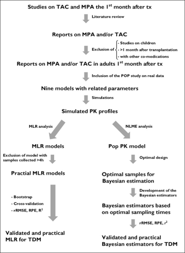
Schema of the statistical approach used for data generation and analysis

MLR models

The simulated dataset was successively and randomly split in two groups: (1) a model building subgroup (test group) comprising 2/3 of patients and a validation subgroup of the remaining patients. This procedure was repeated 20 times. Mean values of regression coefficients estimated during this process were considered as final parameters. Limited sampling strategies were developed to predict MPA and TAC AUC(0,12 h) values, calculated based on the full PK profiles by MLR (JMP/SAS software, SAS, Cary, NC, USA) using various combinations of at most two MPA plasma and TAC blood concentrations determined during the 4 h interval following dosing in the test group. The predicted AUC(0,12 h) from each model was compared with the reference AUC(0,12 h) in the validation subgroup as described below. The reference AUC(0,12 h) was considered to be the AUC(0,12 h) computed by the linear trapezoidal rule [non-compartmental analysis (NCA)]. The best model was additionally evaluated by generating 1000 bootstraps around each estimated parameter [intercept and slope(s)] and calculating the 90% confidence interval (CI) around each parameter, as well as percentiles. Moreover the ability of the final model to predict AUC(0,12 h) computed from observed data was also assessed.

Development of flexible Bayesian estimators

Pop PK modelling

Non-linear mixed effects modelling was performed on the simulated PK profiles by using nonmem and PsN-toolkit for the modelling process [20], and R for graphical analysis. First order (FO) and first order conditional estimation methods with interaction (FOCEI) were used when fitting simulated MPA plasma and TAC blood concentrations. Different structural models were also tested: one, two and three compartment models with first order or zero order absorption, with or without lag time, transit compartment and Erlang absorption models. Pharmacokinetic parameters were estimated by nonmem in terms of zero order (K₀) or first order absorption rate constant (K₁₂), clearance (CL), volumes of distribution (V) of the various compartments and inter-compartmental clearance (Q) using conventional equations. Since oral bioavailability (F) could not be determined, values for CL, V and Q correspond to the ratios CL/F, V/F and Q/F.

The inter-individual variability in the PK parameters (IIV) was modelled using an exponential model and all parameters were initially tested. The value of a parameter in the i^th individual (P_i) was a function of the typical value of the parameter (θ) and of the individual deviation initially given by η_i, representing the inter-patient variability for the i^th patient. The η terms in the population were supposed to be symmetrically distributed, zero-mean random variables with a variance that is estimated as part of the model estimation from Equation 1]:

Equation 1

η terms were maintained in the structural model only when they improved the model based on the decrease of the Bayesian information criterion (BIC) computed as described below.

Additive, proportional and mixed error models were tested for the residual error as shown in equations 2–4:

Equation 2

Equation 3

Equation 4

where Y represents the observed concentration, IPRED is the individual predicted concentration and ε_add and ε_prop are the additive and the proportional error terms on MPA or TAC concentrations, respectively. ε′S were supposed to be symmetrically distributed, zero-mean random variables with variance terms that are estimated as part of the population model-fitting process from equations 2–4.

Model selection only referred to models for which the nonmem minimization process was successful and was based on the following three criteria: (1) the BIC, (2) the plausibility and the precision of parameter estimates and (3) the graphical analysis. The BIC was computed on the model objective function value (OFV), the number of observations used during the modelling process (N_obs) and the number of parameters used (NPAR) as follows:

Equation 5

The models with the lowest BIC were further evaluated. Precision of parameter estimates, expressed as standard error of estimates, was generated by the covariance option within the nonmem program. Goodness of fit plots including predictions and individual predictions vs. observed concentrations, as well as conditional weighted residuals (CWRES) vs. time after dose, were used for model diagnostic purposes.

Selection of the optimal sampling times for Bayesian estimation

This step was performed using Population Experiment Design (PopED) [21]. The criterion to be optimized here is the expected information provided by an experiment i.e. the expectation, over all the possible observations, of the information provided by the experiment performed with a given design in an individual.

The optimality criterion was first optimized with regards to sampling schedule in terms of discrete optimal sampling times in a first time, and optimal sampling windows were estimated around each sampling time subsequently to allow flexibility in the practical clinical use. A loss of efficiency of less than 20% was considered to be an acceptable cost regarding parameter Bayesian estimation [21].

With this approach we studied only one- and two-point designs in each group with sampling times varying between 0 h and 4 h by increments of at least 0.5 h. The three-point design has not been investigated for practical (patient comfort and logistics) reasons.

MAP Bayesian estimation

Bayesian estimation (by the POSTHOC and MAXEVAL = 0 option of the nonmem estimation subroutine) was performed by using the developed POP PK model. The optimal sampling times obtained from the previous step were used. Reference AUC(0,12 h) (obtained by NCA) values were compared with AUC(0,12 h) computed using the Bayesian estimators including optimized sampling times as described below.

Evaluation of predictive performance of AUC(0,12 h) predictors using patients data

Linear regression was performed to evaluate the strength of the correlation between the AUC(0,12 h) values predicted by the various LSS/ Bayesian estimators and the reference AUC(0,12 h) values. The Pearson coefficient of determination r² was one of the criteria to select the best LSS. In addition, predictive performance of the various LSS and agreement between predicted and reference AUC(0,12 h) were assessed as described by Sheiner & Beal [22] and Bland & Altman [23], respectively. Sheiner & Beal described two parameters: (1) the root mean square error (RMSE) to characterize the precision of the model, and the prediction error (PE) to estimate the bias on each difference between predicted and reference AUC(0,12 h). The lower the RMSE and PE values, the better the mode is. Bland & Altman used the 95% CI around the mean relative prediction error (RPE) to assess the predictive performance of the LSS. Equations 6] and 7] display expressions of estimation of relative root mean squared error (rRMSE), RPE and mean relative prediction error (MRPE), respectively. Finally, during the evaluation of predictive performance in this study, a model was considered to display a good predictive performance when, in the validation sample set, the 95% CI around the mean RPE was included between −20% and +20% [7] of the reference MPA AUC(0,12 h) values.

Equation 6

Equation 7

where AUC_ref represents the reference AUC(0,12 h) and AUC_pred the AUC(0.12 h) predicted by the model.

Results

Histograms of distributions of simulated and PK profiles for MPA and TAC are shown in Figure 2. A good concordance between simulations and observations has been obtained showing that the simulation processes were properly performed.

Figure 2.

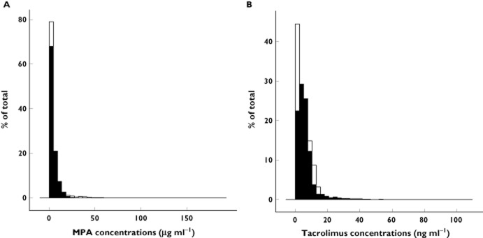
Histograms of simulated (white) and observed (black) mycophenolate (A) and tacrolimus (B) concentrations

Stepwise multiple linear regression analysis was used to select MPA and TAC concentration–time points within the 0 to 4 h post-dose interval that best predicted total exposure. Best model equations in terms of predictive performances [correlation (Pearson r²), accuracy and precision (MRPE, RMSE and bootstraps)] are shown in Tables 1 and 2.

Table 1.

Multiple linear regression models for MPA

Model	Sampling times (h)	Model equation	r2	rRMSE (%)	MRPE (%)
1	1.5, 3.5	16.5 + 4.9 × C1.5 + 6.7 × C3.5	0.82	9	14
2	2, 2.5	21.3 + 6.7 × C2 + 3.3 × C2.5	0.77	11	25
3	1.5, 3	20.6 + 4.7 × C1.5 + 5.5 × C3	0.77	11	27
4	2, 3	23.1 + 6.9 × C2 + 3.7 × C3	0.77	13	29
5	2, 3.5	27.8 + 6.23 × C2 + 4.2 × C3.5	0.77	13	32

MPA, mycophenolic acid; MRPE, mean relative prediction error; rRMSE, relative root mean squared error.

Table 2.

Multiple linear regression models for TAC

Model	Sampling times (h)	Model equation	r2	rRMSE (%)	MRPE (%)
1	3, 3.5	34.1 + 6.1 × C3 + 11.9 × C3.5	0.97	11.5	1.2
2	1.5, 3.5	24.3 + 5.9 × C1.5 + 12.2 × C3.5	0.94	12.3	4.2
3	1.5, 4	26.3 + 6.6 × C1.5 + 11.6 × C4	0.94	12.5	5.4
4	2, 4	25.5 + 8.1 × C2 + 4.5 × C4	0.94	13.1	6.6
5	1, 3.5	31.4 + 5.4 × C1 + 3.5 × C3.5	0.94	13.1	6.7

MPA, mycophenolic acid; MRPE, mean relative prediction error; rRMSE, relative root mean squared error.

Model equation 1], with samples drawn at 1.5 and 3.5 h post-dosing, showed not only the best fit to the MPA AUC(0,12 h) (r² = 0.82), but also better prediction precision and accuracy compared with the other models. Residuals were normally distributed (P values of Shapiro Wilk test were >0.10 for all the parameters).

For TAC, samples drawn at 3 and 3.5 h post-dosing, (model equation 1]) were the best predictor of AUC(0,12 h) (r² = 0.97) and also had the better prediction precision and accuracy compared with the other models. As the aim of the study was to monitor simultaneously MPA and TAC exposure during TDM, the second model (model 2) with samples drawn at 1.5 and 3.5 h post-dose was retained because the sampling times were the same as those of the best model for MPA. Additionally, the predictive performances of this second model were very close to those of the first model.

In order to evaluate the predictive performances of these retained models on the observed patient data, the sample at 3.5 h (not drawn) was considered to be the arithmetic mean of the samples drawn at 3 and 4 h post-dose. The retained models for MPA and TAC also showed acceptable predictive performances for AUC(0,12 h) computed from observed data: r² = 0.66, rRMSE = 24%, MRPE = 17% (95% CI 16.1, 18.4%) and r² = 0.74, rRMSE = 15%, MRPE = 9% (95% CI 8.5, 9.8%) for MPA and TAC, respectively. These performances were also assessed separately for the two different pharmaceutical formulations of MPA and the following results were obtained: r² = 0.62, rRMSE = 29.4%, RPE = 19% (95% CI 18, 20.3%) and r² = 0.71, rRMSE = 17%, RPE = 13% (95% CI 12.2, 14%) for ECMPS and MMF, respectively.

Two compartment disposition models with first order absorption were used to describe MPA and TAC profiles. Parameter values are presented in Table 3. Basic goodness of fit plots are presented in Figures 3 and 4 for MPA and TAC, respectively.

Table 3.

Population pharmacokinetic model characteristics

Parameters	MPA model estimates [RSE]	TAC model estimates [RSE]
θKa (h−1)	2.65 [0.16]	1.68 [0.01]
θTLAG (h)	–	0.045 [0.09]
θV1 (l)	133 [0.18]	221 [0.14]
θV2 (l)	995 [0.13]	520.8 [0.02]
θQ (l h−1)	28.2 [0.06]	21.9 [0.08]
θCL (l h−1)	6.83 [0.05]	3.85 [0.09]
IIV on Ka (%)	142 [0.17]	199 [0.19]
IIV on V1 (%)	108 [0.19]	133 [0.15]
IIV on V2 (%)	168 [0.21]	144 [0.19]
IIV on Q (%)	–	–
IIV on CL (%)	246 [0.19]	185 [0.11]
IIV on TLAG (%)	–	350 [0.24]
εprop	0.49 [0.24]	0.01 [0.23]
εadd (ng ml−1)	0.6 [0.15]	0.97 [038]

CL, clearance; IIV, inter-individual variability; MPA, mycophenolic acid; Q, intercompartmental clearance; RSE, relative standard error of estimates; TLAG, lag time; V₁, volume of central compartment; V₂, volume of peripheral compartment; θ population parameter. ε_prop, coefficient of variation on the proportional term of the residual error. ε_add, standard deviation on the additive term of the residual error.

Figure 3.

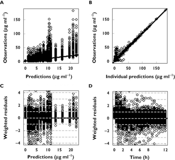
Goodness of fit plots of the population pharmacokinetic model for MPA. (A) observed vs. predicted concentrations, (B) observed vs. individual predicted concentrations, (C) weighted residuals vs. observations and (D) weighted residuals vs. time

Figure 4.

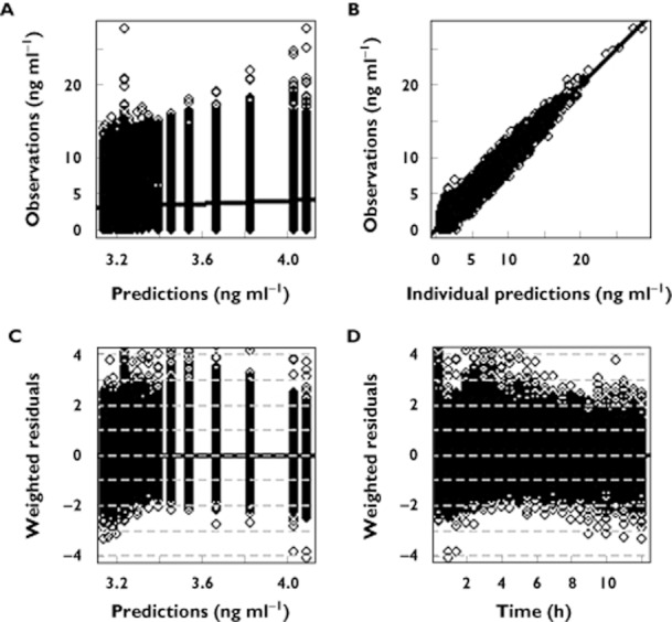
Goodness of fit plots of the population pharmacokinetic model for TAC. (A) observed vs. predicted concentrations, (B) observed vs. individual predicted concentrations, (C) weighted residuals vs. observations and (D) weighted residuals vs. time

The simultaneous optimal sampling times for MPA and TAC Bayesian estimation obtained from optimal sampling design were 1.5 and 3.5 h post-dose.

The results of the estimation of sampling windows around the optimal sampling times showed that drawing samples within the 30 min around the optimal samples did not result in a significant loss of efficiency (>20%) in individual parameter estimation.

Bayesian estimation of PK parameters using the final model parameters as prior information and the optimal sampling times obtained from the preceding step enabled the best prediction of individual MPA and TAC AUC(0,12 h), with satisfactory accuracy and precision as compared with the reference values (r² = 0.90, rRMSE = 11% for MPA and r² = 0.97, rRMSE = 5% for TAC). The Bayesian estimators could therefore be considered to have good predictive performance with regards to the reference AUC(0.12 h). Regressions and Bland & Altman plots for comparisons between reference and Bayesian-predicted AUC(0,12 h) are presented in Figures 5 and 6 for MPA and TAC, respectively. The Bayesian estimators for MPA and TAC also showed acceptable predictive performances for AUC(0,12 h) computed from observed data: r² = 0.75, rRMSE = 11%, MRPE = 12.2% (95% CI 11.5, 12.8%) and r² = 0.83, rRMSE = 7%, MRPE = 8% (95% CI 5.7, 9.4%) for MPA and TAC, respectively. The same performances were also assessed separately for the two different pharmaceutical formulations of MPA and the following results were obtained: r² = 0.71, rRMSE = 13.4%, MRPE = 13.9% (95% CI 12.7, 14.4%) and r² = 0.77, rRMSE = 9.4%, MRPE = 10% (95% CI 8.5, 11.1%) for ECMPS and MMF respectively.

Figure 5.

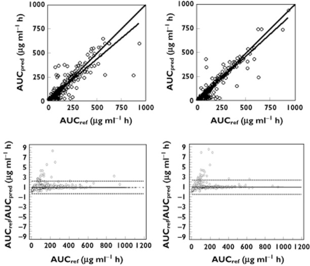
Linear regression (top) and Bland & Altman (bottom) plots of reference AUC(0,12 h) vs. AUC(0,12 h) predicted by the best MLR model (left) and the Bayesian estimator (right) for MPA. : regression line; : identity line

Figure 6.

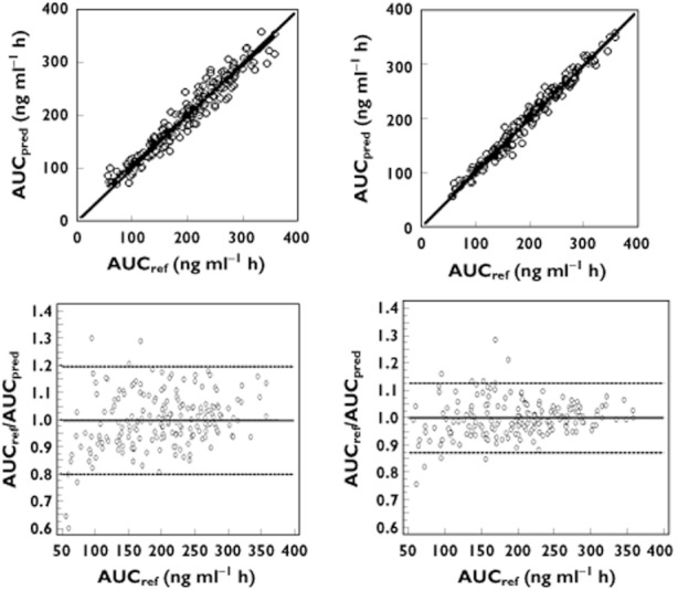
Linear regression (top) and Bland & Altman (bottom) plots of reference AUC₁₂ vs. AUC(0,12 h) predicted by the best MLR model (left) and the Bayesian estimator (right) for TAC. : regression line; : identity line

With the Bayesian estimators only 13 and 5% of the patients had an AUC(0,12 h) < −20% or >+20% of the reference value for MPA and TAC, respectively whereas these levels were 16 and 9% for the corresponding MLR models.

Discussion

Multiple linear regression models and Bayesian estimators have been developed for simultaneous MPA and TAC monitoring within the 4 h following dose administration. The particularity of the tools presented hereby is in their suitability to be used first all along the first month after transplantation, irrespective of the exact post-transplantation period concomitantly or separately for TAC and MPA and secondly their suitability to be used in the absence of additional information on patients' specificity such as genetic polymorphism, bodyweight, markers of kidney or liver function values, other co-medications etc. This is because these tools were developed based on covariate-free models using data from different post-transplantation periods and very heterogeneous groups regarding patient characteristics. Some of the patients' characteristics have been included in the previously published final forms of these models [13–20] and can be used as correction factors or clusters for group dosing. The results regarding covariate selections are, however, not always consistent across trials showing that more research is need to confirm their suitability for clinical use. Therefore the fact that the tools presented here are independent of these characteristics could be perceived as an advantage and at least render them easier to be used in clinical practice.

Several MLR models have been previously published for separate TDM of TAC or MPA [7, 8]. The use of these models could be very demanding for the patients if a TDM is needed for both TAC and MPA since they include different sampling times increasing the number of required samples for both drugs. Since MPA and TAC are often used concomitantly after renal transplantation, there is an interest to find estimators with shared sampling times for MPA and TAC allowing simultaneous dose adjustment for both of the drugs. To the best of our knowledge only one report has presented simultaneous prediction of MPA and TAC AUC(0,12 h) using the MLR approach and it concerns stable patients more than 3 months after transplantation [9]. The present study is, therefore, to the best of our knowledge, the first report proposing tools for simultaneous dose adjustment of MPA and TAC during the first month after kidney transplantation based on their PK.

In the present study, the MLR equations based on plasma/blood concentrations of MPA and TAC obtained 1.5 and 3.5 h post-dose showed the best predictive performance as compared with other sampling times during the validation on simulation data and were in the range of previously published MLR for both MPA and TAC. As expected, these performances were found to be less good when applied to observed data: this can be explained by the fact that the observed data were all collected at day 15 after transplantation whereas simulations were performed from models developed using data collected at different times during the first month after transplantation.

If the model equation based on sampling times at 1.5 and 3.5 h after the dose was found to fit the data well from both formulations of MPA taken together, when considered separately, the predictive performances were more interesting for MMF than EC-MPS when assessed either on simulated data or on observed data. This is consistent with the higher variability in MPA PK after administration of the EC-MPS formulation as compared with the MMF formulation.

The performances for MLR were lower than those of the corresponding Bayesian estimator but still acceptable for both MPA and TAC. Less than 20% of patients had their predicted AUC(0,12 h) outside the acceptable range of ±20% of the reference value. However, unlike MAP Bayesian estimation of AUC(0,12 h), LSS based on MLR require strict adherence to sampling times. Nevertheless, the MLR approach is less demanding regarding statistical computations for its implementation in routine practice than the Bayesian estimation method.

The model equations were validated and the sampling times were restricted to the 4 h time period following immunosuppressant administration. A shorter interval was not possible due to the high variability in the MPA absorption profiles, particularly in the case of EC-MPS administration.

Assuming linear PK for both MPA and TAC the use of the proposed tools for dose adjustment can be done as described in Figure 7 when targeting an exposure in the middle of the therapeutic window i.e. 45 μg ml⁻¹ h for MPA [10] and 180 ng ml⁻¹ h for TAC [1], equations 8] and 9] should be used for MPA and TAC dose adjustment, respectively:

Figure 7.

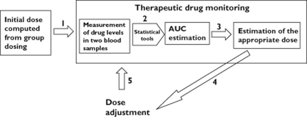
Schematic representation of the procedure for dose adjustment based on the target exposure

Equation 8

Equation 9

In case of need for dose titration, the targeted exposure should be reached after a time delay of around five half-lives (2–5 days for MPA and 2–4 days for TAC), the time delay needed to reach steady-state conditions. A new TDM should not be performed before this delay, which confirms the results of a recently published study on feasibility of MPA TDM early after transplantation and showing an added value for MPA TDM performed every week during the first month after transplantation [24, 25].

Currently, various computer programs are used for dose individualization based on patient concentrations. They generally use algorithms based on MLR or Bayesian estimators. These algorithms vary from one software to another and given that they are based not only on empirical models developed in different settings and groups of patients but also the studies used to develop them were sometimes relatively small and therefore could lack power, their adequate use should only be based on interpolation i.e. each algorithm should only be applicable in the specific case of the patients and settings used to develop it. It can therefore happen that different tools provide conflicting results and the choice between these results will not always be easy. This issue is addressed here since we propose unique tools that can be incorporated in TDM dedicated software and can be appealing in that they are applicable for various settings and patients and can allow MPA and TAC TDM from the same sampling times.

This study was performed using data collected in the first month after transplantation and it is known that in this period after transplantation patients are generally not stable, and the PK variability has been reported to be the highest for MPA and TAC [2, 3]. TDM is therefore of importance in this period for both drugs and the estimators developed in this study could be included in TDM dedicated PK computer programs. Models developed in paediatrics, models for MPA in patients not co-medicated with TAC or for TAC in patients not co-medicated with MPA and models developed for periods later than 1 month after transplantation were not retained because the focus of this study was to develop help for dose individualization in adult patients co-medicated with TAC and MPA based on shared samples (same sampling times) in the early period after transplantation. We considered this period to be the first month after transplantation. Moreover, patient age, co-medications and time post-transplantation have been reported to influence both TAC and MPA PK.

In conclusion, multiple linear regression models and Bayesian estimators have been developed for simultaneous MPA and TAC TDM in the 4 h following dose administration. The MLR models were validated by bootstrap and cross-validation. The Bayesian estimator was designed based on optimality and also validated. They could therefore be used for routine TDM.

Competing Interests

All authors have completed the Unified Competing Interest form at http://www.icmje.org/coi_disclosure.pdf (available on request from the corresponding author) and declare no support from any organization for the submitted work; no financial relationships with any organizations that might have an interest in the submitted work in the previous 3 years and no other relationships or activities that could appear to have influenced the submitted work.

References

- 1.Wallemacq P, Armstrong VW, Brunet M, Haufroid V, Holt DW, Johnston A, Kuypers D, Le Meur Y, Marquet P, Oellerich M, Thervet E, Toenshoff B, Undre N, Weber LT, Westley IS, Mourad M. Opportunities to optimize tacrolimus therapy in solid organ transplantation: report of the European consensus conference. Ther Drug Monit. 2009;31:139–152. doi: 10.1097/FTD.0b013e318198d092. [DOI] [PubMed] [Google Scholar]
- 2.Staatz CE, Tett SE. Clinical pharmacokinetics and pharmacodynamics of mycophenolate in solid organ transplant recipients. Clin Pharmacokinet. 2007;46:13–58. doi: 10.2165/00003088-200746010-00002. [DOI] [PubMed] [Google Scholar]
- 3.Staatz CE, Tett SE. Clinical pharmacokinetics and pharmacodynamics of tacrolimus in solid organ transplantation. Clin Pharmacokinet. 2004;43:623–653. doi: 10.2165/00003088-200443100-00001. [DOI] [PubMed] [Google Scholar]
- 4.Staatz CE, Willis C, Taylor P, Tett SE. Population pharmacokinetics of tacrolimus in adult kidney transplant recipients. Clin Phamacol Ther. 2002;72:660–669. doi: 10.1067/mcp.2002.129304. [DOI] [PubMed] [Google Scholar]
- 5.Benkali K, Prémaud A, Picard N, Rérolle JP, Toupance O, Hoizey G, Turcant A, Villemain F, Le Meur Y, Marquet P, Rousseau A. Tacrolimus pharmacokinetic-pharmacogenetic analysis and Bayesian estimation in renal transplant recipients. Clin Pharmacokinet. 2009;48:805–816. doi: 10.2165/11318080-000000000-00000. [DOI] [PubMed] [Google Scholar]
- 6.Hale MD, Nicholls AJ, Bullingham Hené R, Hoitsma A, Squifflet JP, Weimar W, Vanrenterghem Y, Van de Woude FJ, Verpooten GA. The pharmacokinetic-pharmacodynamic relationship for mycophenolate mofetil in renal transplantation. Clin Pharmacol Ther. 1999;64:672–683. doi: 10.1016/S0009-9236(98)90058-3. [DOI] [PubMed] [Google Scholar]
- 7.Hale MD, Nicholls AJ, Bullingham RE, Hené R, Hoitsma A, Squifflet JP, Weimar W, Vanrenterghem Y, Van de Woude FJ, Verpooten GA. Maximum a posteriori Bayesian estimation of mycophenolic acid pharmacokinetics in renal transplant recipients at different postgrafting periods. Ther Drug Monit. 2005;27:354–361. doi: 10.1097/01.ftd.0000162231.90811.38. [DOI] [PubMed] [Google Scholar]
- 8.Figurski MJ, Nawrocki A, Pescovitz MD, Bouw R, Shaw LM. Development of a predictive limited sampling strategy for estimation of mycophenolic acid area under the concentration time curve in patients receiving concomitant sirolimus or cyclosporine. Ther Drug Monit. 2008;30:445–455. doi: 10.1097/FTD.0b013e318180c986. [DOI] [PubMed] [Google Scholar]
- 9.Mathew BS, Fleming DH, Jeyaseelan V, Chandy SJ, Annapandian VM, Subbanna PK, John GT. A limited sampling strategy for tacrolimus in renal transplant patients. Br J Clin Phamacol. 2008;66:467–472. doi: 10.1111/j.1365-2125.2008.03251.x. [DOI] [PMC free article] [PubMed] [Google Scholar]
- 10.Le Meur Y, Büchler M, Thierry A, Caillard S, Villemain F, Lavaud S, Etienne I, Westeel PF, Hurault de Ligny B, Rostaing L, Thervet E, Szelag JC, Rérolle JP, Rousseau A, Touchard G, Marquet P. Individualized mycophenolate mofetil dosing based on drug exposure significantly improves patient outcomes after renal transplantation. Am J Transplant. 2007;7:2496–2503. doi: 10.1111/j.1600-6143.2007.01983.x. [DOI] [PubMed] [Google Scholar]
- 11.Musuamba FT, Di Fazio V, Van Bist R, Wallemacq P. A fast ultra performance liquid chromatography for simultaneous quantification of mycophanolic acid and its phenol- and acyl glucuronides in human plasma. Ther Drug Monit. 2009;31:110–115. doi: 10.1097/FTD.0b013e318191897d. [DOI] [PubMed] [Google Scholar]
- 12.Alak AM. Measurement of tacrolimus (FK506) and its metabolites: a review of assay development and application in therapeutic drug monitoring and pharmacokinetic studies. Ther Drug Monit. 1997;19:338–351. doi: 10.1097/00007691-199706000-00016. [DOI] [PubMed] [Google Scholar]
- 13.Benkali K, Rostaing L, Premaud A, Woillard JB, Saint-Marcoux F, Urien S, Kamar N, Marquet P, Rousseau A. Population pharmacokinetics and Bayesian estimation of tacrolimus exposure in renal transplant recipients on a new once-daily formulation. Clin Pharmacokinet. 2010;49:683–692. doi: 10.2165/11535950-000000000-00000. [DOI] [PubMed] [Google Scholar]
- 14.Antignac M, Barrou B, Farinotti R, Lechat P, Urien S. Population pharmacokinetics and bioavailability of tacrolimus in kidney transplant patients. Br J Clin Pharmacol. 2007;64:750–757. doi: 10.1111/j.1365-2125.2007.02895.x. [DOI] [PMC free article] [PubMed] [Google Scholar]
- 15.Musuamba FT, Mourad M, Haufroid V, Demeyer M, Capron A, Delattre IK, Delaruelle F, Wallemacq P, Verbeeck RK. A simultaneous d-optimal designed study for population pharmacokinetic analyses of mycophenolic acid and tacrolimus early after renal transplantation. J Clin Pharmacol. 2012;52:1833–1843. doi: 10.1177/0091270011423661. [DOI] [PubMed] [Google Scholar]
- 16.Staatz CE, Duffull SB, Kiberd B, Fraser AD, Tett SE. Population pharmacokinetics of mycophenolic acid during the first week after renal transplantation. Eur J Clin Pharmacol. 2005;61:507–516. doi: 10.1007/s00228-005-0927-4. [DOI] [PubMed] [Google Scholar]
- 17.de Winter BC, van Gelder T, Sombogaard F, Shaw LM, van Hest RM, Mathot RA. Pharmacokinetic role of protein binding of mycophenolic acid and its glucuronide metabolite in renal transplant recipients. J Pharmacokinet Pharmacodyn. 2009;36:541–564. doi: 10.1007/s10928-009-9136-6. [DOI] [PMC free article] [PubMed] [Google Scholar]
- 18.Cremers S, Schoemaker R, Scholten E, den Hartigh J, König-Quartel J, van Kan E, Paul L, de Fijter J. Characterizing the role of enterohepatic recycling in the interactions between mycophenolate mofetil and calcineurin inhibitors in renal transplant patients by pharmacokinetic modelling. Br J Clin Pharmacol. 2005;60:249–256. doi: 10.1111/j.1365-2125.2005.02398.x. [DOI] [PMC free article] [PubMed] [Google Scholar]
- 19.Sherwin CM, Fukuda T, Brunner HI, Goebel J, Vinks AA. The evolution of population pharmacokinetic models to describe the enterohepatic recycling of mycophenolic acid in solid organ transplantation and autoimmune disease. Clin Pharmacokinet. 2011;50:1–24. doi: 10.2165/11536640-000000000-00000. [DOI] [PMC free article] [PubMed] [Google Scholar]
- 20.Lindbom L, Pihlgren P, Jonsson EN. PsN-Toolkit–a collection of computer intensive statistical methods for non-linear mixed effect modeling using NONMEM. Comput Methods Programs Biomed. 2005;79:241–257. doi: 10.1016/j.cmpb.2005.04.005. [DOI] [PubMed] [Google Scholar]
- 21.Foracchia M, Hooker A, Vicini P, Ruggeri A. POPED, a software for optimal experiment design in population kinetics. Comput Methods Programs Biomed. 2004;74:29–46. doi: 10.1016/S0169-2607(03)00073-7. [DOI] [PubMed] [Google Scholar]
- 22.Sheiner LB, Beal SL. Some suggestions for measuring predictive performance. J Pharmacokinet Biopharm. 1981;9:503–512. doi: 10.1007/BF01060893. [DOI] [PubMed] [Google Scholar]
- 23.Bland JM, Altman DG. Statistical methods for assessing agreement between two methods of clinical measurement. Lancet. 1986;1:307–310. [PubMed] [Google Scholar]
- 24.Saint-Marcoux F, Vandierdonck S, Prémaud A, Debord J, Rousseau A, Marquet P. Large scale analysis of routine dose adjustments of mycophenolate mofetil based on global exposure in renal transplant patients. Ther Drug Monit. 2011;33:285–294. doi: 10.1097/FTD.0b013e31821633a6. [DOI] [PMC free article] [PubMed] [Google Scholar]
- 25.Tett SE, Saint-Marcoux F, Staatz CE, Brunet M, Vinks AA, Miura M, Marquet P, Kuypers DR, van Gelder T, Cattaneo D. Mycophenolate, clinical pharmacokinetics, formulations, and methods for assessing drug exposure. Transplant Rev. 2011;25:47–57. doi: 10.1016/j.trre.2010.06.001. [DOI] [PubMed] [Google Scholar]