An efficient framework for optimization and parameter sensitivity analysis in arterial growth and remodeling computations

Abstract

Computational models for vascular growth and remodeling (G&R) are used to predict the long-term response of vessels to changes in pressure, flow, and other mechanical loading conditions. Accurate predictions of these responses are essential for understanding numerous disease processes. Such models require reliable inputs of numerous parameters, including material properties and growth rates, which are often experimentally derived, and inherently uncertain. While earlier methods have used a brute force approach, systematic uncertainty quantification in G&R models promises to provide much better information. In this work, we introduce an efficient framework for uncertainty quantification and optimal parameter selection, and illustrate it via several examples. First, an adaptive sparse grid stochastic collocation scheme is implemented in an established G&R solver to quantify parameter sensitivities, and near-linear scaling with the number of parameters is demonstrated. This non-intrusive and parallelizable algorithm is compared with standard sampling algorithms such as Monte-Carlo. Second, we determine optimal arterial wall material properties by applying robust optimization. We couple the G&R simulator with an adaptive sparse grid collocation approach and a derivative-free optimization algorithm. We show that an artery can achieve optimal homeostatic conditions over a range of alterations in pressure and flow; robustness of the solution is enforced by including uncertainty in loading conditions in the objective function. We then show that homeostatic intramural and wall shear stress is maintained for a wide range of material properties, though the time it takes to achieve this state varies. We also show that the intramural stress is robust and lies within 5% of its mean value for realistic variability of the material parameters. We observe that prestretch of elastin and collagen are most critical to maintaining homeostasis, while values of the material properties are most critical in determining response time. Finally, we outline several challenges to the G&R community for future work. We suggest that these tools provide the first systematic and efficient framework to quantify uncertainties and optimally identify G&R model parameters.

1. Introduction

Arterial development, maintenance, disease progression, and responses to injury all result from the balanced or imbalanced turnover of cells and extracellular matrix under mechanical loading. Computational models of growth and remodeling (G&R) have been developed to study long-term responses of vessels to sustained alterations in hemodynamic and mechanical loads [1–4]. Since experiments to elucidate G&R responses can involve long periods, simulations can augment experimental knowledge and help to identify and test hypotheses of growth or remodeling responses. Additionally, computer simulations can provide detailed information on wall thickness, mass fractions of constituents, stress–strain behaviors, and lumen size, which are not always easily obtained in vivo.

Two main classes of G&R models are [5–10]: (a) models that evolve stress-free configurations of each constituent and assemble them into a composite body through an elastic deformation, or (b) models that evolve a mixture of constituents, in which new components are added at a prestretched state. We adopt the second approach, the constrained mixture model, which requires three constitutive equations for individual constituents: stored energy functions, production functions, and survival functions. Valentin and Humphrey [11] showed that stress-mediated production and constituent-specific deposition stretches are essential for simulating realistic arterial adaptations, but the requisite constitutive equations require many parameters to capture accurate behaviors [3,12]. Therefore, there is a pressing need for rigorous methods to quantify uncertainties and to systematically choose optimal parameters.

Input uncertainties to G&R simulations may propogate nonlinearly to the outputs, resulting in significant output uncertainties for some quantities of interest. Prior sensitivity studies of Valentin and Humphrey [13] used uniform sampling methods in which one or two parameters were varied at a time while keeping the others fixed. This approach quickly becomes intractable for the large number of parameters required to describe arterial G&R. Our aim is to quantify and compare these output uncertainties for multiple parameters and to evaluate the robustness of the simulation output for different scenarios. In certain cases, the range of possible inputs is large enough that we use optimization to identify a set of input parameters leading to a known output response. Through a combination of these two tools, we aim to improve the reliability of G&R simulations.

The stochastic collocation method has been used for uncertainty quantification in fluid mechanics, solid mechanics, heat transfer, and similar applications [14–16]. Sparse grid collocation approaches have been particularly successful for computationally expensive problems, offering an alternative to more expensive Monte-Carlo methods. Adaptive collocation methods further extend traditional methods, while maintaining scalability and convergence. Such methods have been developed recently for uncertainty quantification in simulations of abdominal aortic aneurysms, the Fontan surgery, and bypass graft surgery [15]. With this method, we can place error bars and confidence intervals on simulation outputs given a range of input values.

In cases for which model parameters are unknown, optimization offers a systematic method for identifying values that lead to expected behaviors. The surrogate management framework (SMF) is a robust derivative-free algorithm developed for simulation- based-optimization [17]. This method has been used in cardiovascular examples such as optimal branching of arteries [18], the Fontan surgery [19], and bypass graft surgeries [20,14,21]. In this paper, we use the SMF with Kriging surrogate functions to accelerate the search process.

The goals of this paper are twofold: (a) to perform a systematic and rigorous parameter sensitivity study of G&R simulations of normal arterial adaptations to modest changes in blood pressure and flow, and (b) to use a formal optimization procedure to identify a set of optimal parameter values that yield expected G&R responses. First, we test robustness by evaluating the sensitivity of outputs of G&R simulations resulting from uncertainty in material parameters. Rigorous parametric studies such as this can guide future work by identifying critical regions for further experimental studies. Second, we use optimization to select material property values in cases when experimental data are wanting. Optimal material properties insure that homeostatic conditions can be restored over a range of loading conditions. We compute sensitivity contours and confidence intervals to test the credibility of predicted outcomes. The non-intrusive nature of the optimization and uncertainty quantification algorithms makes integration of these tools with the G&R framework particularly attractive. Though we illustrate the proposed tools for a basilar artery, the framework is sufficiently general to be extended to other vascular applications. Whenever available, experimental data should be added as constraints or into the cost function of our framework.

2. Computational framework for growth and remodeling

The arterial wall is assumed to consist initially of elastin (oriented in axial and circumferential directions), four collagen fiber families (at angles of 0°, 90°, 45° and 135° relative to axial), and circumferentially oriented smooth muscle cells (SMC). We assume that the elastin does not turn over during short periods of adaptation, since it is produced during the perinatal period, cross-linked, and stretched elastically during development; the collagen and smooth muscle are allowed to turnover continuously in evolving configurations, however.

Arterial growth and remodeling, leading to adaptation herein, is simulated using previously validated models [12,13]. Briefly, we assume that G&R is a quasi-static process whereby intramural and wall shear stresses can be computed via

$${\sigma }_{\theta ,\theta }=\frac{Pa}{h},{\sigma }_{zz}=\frac{f}{\pi h(2a+h)},{\tau }_w=\frac{4\mu Q}{\pi a^3},$$ (1)

where P and Q are mean blood pressure and volumetric flow rate, f is the applied axial load, and a and h are inner radius and wall thickness. These equilibrium/steady state solutions for laminar flow of a constant viscosity fluid (μ) within a thin-walled cylindrical vessel provide the requisite values of stress for the G&R model. In particular, constitutively:

$${\sigma }_{\theta ,\theta }=\frac{1}{{\lambda }_z}\frac{\partial W}{\partial {\lambda }_{\theta }}+{\sigma }_{\theta \theta }^{\text{act}}\text{and}{\sigma }_{zz}=\frac{1}{{\lambda }_{\theta }}\frac{\partial W}{\partial {\lambda }_z},$$ (2)

where (λ_θ, λ_z) are mean circumferential and axial wall stretches, ${\sigma }_{\theta \theta }^{\text{act}}$ is the active muscle contribution, and W is the stored energy function, which for a constrained mixture is given by W = ΣW^k where

$$W^k(s)=\frac{M^k(0)}{\rho (s)}{Q}^k(s){\widehat{W}}^k({\lambda }_{n(0)}^k)+{\int }_0^s\frac{m^k(\tau )}{\rho (s)}{q}^k(\tau ,s){\widehat{W}}^k({\lambda }_{n(\tau )}^k)d\tau .$$

where $M_0^k$ is the initial mass density for constituent k (=e for elastin, c for any of four families of collagen fibers, or m for the smooth muscle), Q^k(s) ∈ [0, 1] is the fraction of constituent k that remains at G&R time s that was produced at time 0,m^k(τ) is a mass density production, q^k(τ, s) ∈ [0, 1] is the fraction of constituent k that remains at G&R time s that was produced at time τ ∈ [0, s], ${\widehat{W}}^k\left({\lambda }_{n(\tau )}^k\right)$ is the energy stored in constituent k, which depends on the constituent stretch relative to its natural configuration n(τ). Finally, ρ(s) is the mass density of the entire wall, which is assumed to remain constant.

Fundamental to this G&R framework is specification of the three classes of constituent-specific constitutive relations: Ŵ^k, m^k and q^k. Consistent with prior implementations [12,13], we let

$${\widehat{W}}^e({\lambda }_{n(\tau )}^e)=c^e\left({\lambda }_{\theta }^{e^2}+{\lambda }_z^{e^2}+\frac{1}{{\lambda }_{\theta }^{e^2}{\lambda }_z^{e^2}}-3\right),$$ (3)

for elastin and

$${\widehat{W}}^j({\lambda }_{n(\tau )}^j)=c_1^j\mathit{exp}\left(c_2^j{({\lambda }^{j^2}-1)}^2-1\right),$$

for collagen (j = c) or smooth muscle (j = m). It should be noted that these constituent-specific stretches differ due to their deposition at different homeostatic values $G_h^k$, namely

$${\lambda }_{n(\tau )}^k(s)=G_h^k\frac{\lambda (s)}{\lambda (\tau )},$$ (4)

where λ(τ) is the stretch experienced by the artery in the direction of interest relative for τ ∈ [0, s].

Finally, note that we assume a stress-dependent production, namely

$$m^c=m_0^c(1+K_1^c\mathrm{\Delta }\sigma -K_2^c\mathrm{\Delta }{\tau }_w),$$ (5)

$$m^m=m_0^m(1+K_1^m\mathrm{\Delta }\sigma -K_2^m\mathrm{\Delta }{\tau }_w),$$ (6)

where $m_0^k$ are basal values, $K_1^k$ and $K_2^k$ are gain type parameters and

$$\mathrm{\Delta }\sigma =\frac{\sigma -{\sigma }_h}{{\sigma }_h},\mathrm{\Delta }{\tau }_w=\frac{{\tau }_w-{\tau }_w^h}{{\tau }_w^h},$$ (7)

are normalized intramural and wall shear stress differences, with superscript h denoting the homeostatic value. Hence, collagen and smooth muscle production will be increased in response to an increase in intramural stress or a decrease in wall shear stress (since constrictors are mitogens) and vice versa. The ratio of vasoconstrictors to vasodilators C_ratio is this important. We also let m^e ≡ 0 since elastin is produced only in the perinatal period. The survival functions Q^k and q^k are assumed to follow first order kinetics as in [12,13]. Herein, however, we will focus on the parameters c^e, $c_1^j,c_2^j$ (wall properties), $G_h^e$ and $G_h^c$ (constituent prestretches), and $K_1^k$ and $K_2^k$ (production rates).

The G&R problem is thus solved by insuring that equilibrium via equality of intramural stresses computed via Eqs. (1) and (2). Toward this end, we allow the hemodynamics to be perturbed from homeostatic pressure and flow (P_h and Q_h) via P = γP_h and Q = εQ_h, where (γ, ε) are scaling parameters. Hence, using a Newton–Raphson method (see [11]), we compute the evolving mass and radius a at each G&R time s and then calculate thickness h. The assumption is that a full adaptation will yield a = ε ^1/3a_h and h = γε^1/3h_h [11]. Failure to evolve radius and wall thickness in this way is termed sub-optimal, or in extreme cases, mal-adaptation.

We split the parameters

$$p=\left[p^K{p}^G{p}^c\right],$$

into three groups: (i) gain parameters p^K (4 components), (ii) material parameters $c_1^k$ and $c_2^k$ (10 components) denoted by p^c, and (iii) pre-stretch parameters $G_h^c$ and $G_h^m$ (2 components) denoted by p^G, respectively.

The set of 10 material parameters p^c (2 for each collagen fiber family and 2 for the SMC) reduces to 6 independent components if we impose material equilibrium at the start of the simulations and assume that the collagen fiber families for orientations 45° and 135° are the same. A schematic of the framework and parameters of interest is shown in Fig. 1.

Fig. 1.

Schematic of the G&R framework showing the evolution of arterial geometry and the important parameters which are either stochastic (p^c) or optimized (p^K, p^G).

3. Parameter sensitivity study for G&R simulations

Choice of an uncertainty quantification scheme in a simulation-based system depends on both scalability and degree of intrusiveness [22,16,23]. Techniques such as Monte-Carlo [24], quasi Monte-Carlo, and Markov Chain Monte Carlo are sampling algorithms that have poor scalability and cannot be reasonably applied to expensive simulation problems. Polynomial chaos methods offer improved convergence, but require significant intrusion into the solver code. Improved scalability can be achieved with stochastic collocation algorithms, in which a stochastic space is constructed by considering uncertain parameters as an additional dimension [22,25,23,16,25]. This technique combines the exponential convergence rates of the generalized polynomial chaos scheme with the non-intrusive nature of Monte-Carlo techniques.

3.1. Collocation methods

The process of uncertainty quantification using collocation uses the following steps: (i) a set of collocation points is generated, (ii) simulations are run at each point, and (iii) statistics are computed such as probability density function (PDF) and confidence intervals. The level of refinement in the collocation grid is increased in a hierarchical manner to achieved convergence of the statistics. The theory behind collocation and how it can be applied is briefly described below.

The parametric space is approximated using mutually orthogonal interpolating polynomials . A function g(ξ) is then represented in the parametric space as g(ξ) = Σ_ig(ξ_i) (ξ), the subscripts indicating a specific point in the parametric space. We assume g(ξ) is in the space of functions with continuous n^th order derivatives. The interpolating polynomials have the property that (ξ_j) = δ_ij where δ_ij = 1 if i = j and is zero otherwise, hence they are required to pass exactly through the points. This property is necessary for simulation-based collocation, where each simulation corresponds to a specific collocation point.

To choose the collocation points in one-dimension, ξ_j, one can use 1D quadrature rules (such as Chebyshev nodes for Lagrange polynomials). The simplest means for extension to multiple stochastic dimensions is the tensor-product rule, however this results in poor scalability. The Smolyak sparse grid algorithm with 1D nested Chebyshev nodes [26,22,23] is used here to identify collocation points in a multi-dimensional space. Because we deal with arbitrary continuous PDF’s and are interested in higher order statistical moments, techniques such as analysis of variance and design of experiments are not applicable here [27].

We use the collocation technique both to represent a quantity of interest over multiple parameters and to quantify uncertainty. We define the space of parameters (for each j above) as ξ = [ξ¹, ξ², …, ξ^N] where each ξⁱ ∈ [0, 1] is normalized. Transformations using inverse cumulative distribution functions are used to map ξ to physical variables.

Convergence

In Smolyak sparse grid collocation, the depth of interpolation [28] defines a hierarchy of refinement levels, each requiring more function evaluations. Error indicators are computed for each depth of interpolation. Increasing depth of interpolation insures convergence of the output statistics. In practice, the depth of interpolation allows flexibility in implementation because the level can be chosen according to computational expense and desired tolerances. We have demonstrated that Lagrange interpolates converge quickly with a small depth of interpolation in several cardiovascular blood flow examples [15].

Adaptive collocation

To further reduce computational cost, collocation points can be chosen adaptively, as shown in our recent work [15,20]. A hierarchical error indicator is defined that compares the current to the next collocation level. By only adding points in regions of the function that need additional refinement, a cost savings of up to 50% is achieved [15]. The adaptive criterion is decided based on the contribution of the solution at a collocation point, and aims to reduce the cost of performing additional simulations at regions where variability is small. The adaptivity criterion is linked to the quantity of interest (QOI). In the case of multiple quantities of interest, we envision two different approaches: (a) use a superset of collocation nodes resulting from using each QOI individually to obtain the adaptive collocation nodes or (b) use a weighted sum of the QOIs (the weighting has to be determined based on the problem and QOIs).

Uncertainty quantification

By sampling the parametric space, ξ (i.e. the results of simulations at all collocation points and their interpolated values), we quantify the PDF, confidence intervals, and higher order statistical moments [14,15]. This approach provides a measure of the sensitivity of quantities of interest to stochastic variables.

3.2. Problem definition: effect of collagen and smooth muscle cell turnover on arterial adaptations

Our first goal is to systematically quantify the effect of moderate changes in parameter values on arterial G&R predictions. In particular, we examine the effect of two gain parameters controlling arterial adaptation, namely, turnover of collagen fibers and smooth muscle cells. We maintain the flow rate at its homeostatic value (i.e. ε = 1) and increase pressure by 50% (i.e. γ = 1.5), keeping values of the material parameters, p^G and p^c, fixed. Assuming mechanics of a thin cylinder with circular lumen and parabolic velocity profile, the thickness and radius of the artery will change according to h = ε^1/3γh_h and a = ε^1/3a_h to restore intramural stress and shear stress to their homeostatic values. The outputs are gathered after sufficient adaptation time (500 days).

In all examples, we assume that the vessel has the homeostatic radius and thickness of a rabbit basilar artery. For a homeostatic pressure of 93 mm Hg, the target intramural and wall shear stresses are σ^h = 100 kPa and ${\tau }_w^h=5.06\text{Pa}$. With a homeostatic radius of 1.42 mm, the homeostatic thickness and flow rate are calculated as 0.176 mm and 3.075 ml/s, respectively. The values for other parameters were taken from Valentin et al. [12].

3.3. Interpolation results

3.3.1. Two dimensional interpolation results

First, we illustrate the adaptive collocation method on a two-dimensional problem. We fix $K_1^c=K_2^c$ and $K_1^m=K_2^m$, and study the dependence of the predicted radius and thickness on perturbations to p^K. For comparison, we construct a parameter space representation of the adapted radius and thickness using three methods: tensor grid collocation, sparse grid collocation, and adaptive sparse grid collocation (Fig. 2).

Fig. 2.

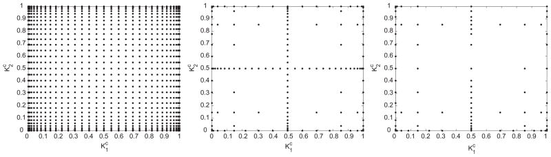
Collocation points for the 2-dimensional interpolation problem (from left) full tensor product interpolation using Clenshaw Curtis abscissas, isotropic Smolyak sparse

The number of simulations needed for two dimensional interpolation with each method are 1000, 200 and 70, respectively. The difference in computational requirements between the three methods increases with dimension. By extrapolation, for a 10 dimensional problem, we will need roughly 10⁷, 10⁵ and 1000 simulations respectively. This scaling also depends on the problem and for a different scenario (e.g. carotid artery or saphenous vein in an artery), it is possible that a non-adapted solution is needed to obtain an accurate solution.

Fig. 3 shows the dependence of the predicted thickness and radius on $K_1^c$ and $K_1^m$ after 500 days of adaptation. For most combinations of $K_1^c$ and $K_1^m$, homeostatic stresses were restored within 500 days. In the neighborhood of K^c = K^m = 0, however, the artery was unable to add sufficient material in response to the pressure increase. Hence, the radius increased and thickness decreased in an unbounded manner, implying that changing geometry alone was insufficient to restore the homeostatic state. This behavior has been observed in previous work [13,11], and serves as a verification of the interpolation method.

Fig. 3.

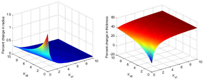
The percent change in final radius and thickness relative to homeostatic values plotted against 2D parameter space. The adaptation is thus robust except for values of $K_1^c$ and $K_2^c$ near zero, which reveals the necessity of stress-mediated turnover.

3.3.2. Five dimensional interpolation results

Next, we employed the stochastic collocation framework for five parameters, p^K and C_ratio. Collocation points were chosen using the adaptive sparse grid method and G&R simulations were performed for each. As shown in Table 1, the adaptive sparse grid collocation method (e.g. right panel in Fig. 2) results in significant computational savings over the Smolyak sparse grid method; it scales almost linearly compared to the polynomial scaling of the Smolyak sparse grid and exponential scaling of the tensor product grid method. By extrapolation, the number of simulations needed for 10 dimensions (at level 3) would be 243, 5900 and 6.4e7, implying that the adaptive algorithm could outperform Smolyak sparse grid by an order of magnitude.

Table 1.

Comparison of the number of simulations needed for the tensor product grids (exponential), Smolyak sparse grid (non-linear) and the adaptive sparse grid (linear).

Level (mesh refinement)	Tensor product	Sparse grid	Adaptive SG
3	75 (~ 104)	180	103
4	155(~ 105)	801	148
5	315(~ 107)	2433	240

Fig. 4 shows predicted changes in radius over a five-parameter space, projected in two dimensions. In the absence of stress-mediated collagen turnover (i.e. K_c = 0), the model cannot maintain or restore homeostatic values. Instead, we must have K_c > 2 for the model to adapt homeostatically over the aforementioned range of ε and γ values. We also evaluated the relative sensitivity to different parameters. For instance, variability of output with respect to K_c is much higher than that due to C_ratio. Fig. 4 shows the dependence of arterial radius on both K_m1 and C_ratio, implying that varying each parameter individually, while keeping the others constant, may not be sufficient to reveal the complex response of the arteries to sustained alterations in biomechanical loading.

Fig. 4.

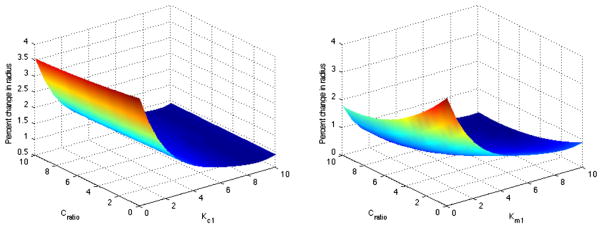
Change in radius as a function of both C_ratio and (left) K_c and (right) K_m.

4. Optimal arterial adaptations under different loading conditions

4.1. Optimization method

Two general classes of optimization techniques are available for simulation-based optimization problems: gradient-based and derivative-free. Evaluation of gradients in simulation based optimization rely on either finite difference approximation or solving an auxiliary problem (either a sensitivity equation or adjoint problem). These techniques are subject to noise and/or require substantial additional computational cost. Derivative-free techniques, on the other hand, rely only on the solution of the direct problem and can be used with a black-box computational solver.

The method we use in this paper (the Surrogate Management Framework, SMF) belongs to a general class of pattern search optimization methods [17]. Pattern search optimization methods are derivative-free, and generate potential points based on coordinate search, often together with a surrogate function that accelerates convergence. An advantage of the SMF optimization scheme is that it has a well-established convergence theory and offers a flexible choice of surrogate function that can, if required, be tailored to the problem. Deterministic SMF has been used successfully in unsteady fluid mechanics problems [30], bio-fluid mechanics [18], surgical design [19], helicopter rotor blade design [31], and multi-objective liquid-rocket injector design [32].

The algorithm proceeds using a combination of SEARCH and POLL steps. All points evaluated are required to lie on a mesh, which can be refined or coarsened as the algorithm proceeds. In the POLL step, which is necessary and sufficient for convergence, a positively spanning basis is identified around the current best design point. A positive basis is defined as a set in which all elements in the space can be generated through a positive linear combination of the basis vectors. New trial design points are selected by performing function evaluations along these directions with a specified step size. There are several methods for generating POLL sets, including generalized pattern search and mesh adaptive direct search (MADS). In this paper, we employ the MADS method because of it’s superior convergence properties. Using the MADS method, the magnitude of the step size depends on a poll size parameter Δ^p, which can be different from the discretization (mesh size) of the parameter space Δ^m [17] as long as all points lie on the same mesh.

The SEARCH step, which is not strictly required for convergence, accelerates convergence by using a Kriging surrogate function. This function is updated with each point that is evaluated. Because optimization can be performed on the surrogate function for near-zero computational cost, new trial designs can be generated by finding minima of the surrogate function. When the SEARCH step fails to give an improved design variable, a POLL step is performed. If the POLL step also fails, the parameter space mesh is refined until a preset threshold is reached.

For applications presented in this paper, we normalized the initial grid size Δ^m, and terminated when Δ^m = 1/16. Fig. 5 shows a schema of the optimization method. The optimization algorithm was run in Matlab using the DACE package for Kriging [33]. Similar pattern search methods can be implemented using open source codes available in Matlab and C++ [34]. While we have implemented an unconstrained optimization method in this work, these methods can be extended to include constraints in a straightforward manner, as shown in prior work [35].

Fig. 5.

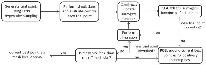
A schema of the derivative-free SMF optimization method.

4.2. Arterial adaptation: cost function definition

A G&R parameter set is considered optimal when the output reaches a specified objective, which here corresponds to reaching a homeostatic state. There are multiple ways to define a multi-objective problem. Two main approaches are - (a) using a weighted sum of the different objective functions including cross-correlating (product-like) terms and (b) constructing a pareto front to quantify trade-offs between different objective functions. In both of these approaches, the weighting of the different terms plays an important role in estimating the final optima. Here, we define a stress-based cost function as:

$$\mathcal{J}=\mathrm{\Delta }{\sigma }_c^2+\mathrm{\Delta }{\sigma }_m^2+\mathrm{\Delta }{\tau }_w^2,$$

where $\mathrm{\Delta }{\sigma }_m={\sigma }^m/{\sigma }_h^m-1,\mathrm{\Delta }{\sigma }_c={\sigma }_c/{\sigma }_h^c-1$, and $\mathrm{\Delta }{\tau }_w={\tau }_w/{\tau }_w^h-1$, such that each term is normalized by its homeostatic value. The inputs to the problem are the perturbation from the homeostatic flow and pressure, parametrized by ε and γ respectively. The goal is to find the optimal parameters p^G, p^K, such that we find min (p^G, p^K ; ε, γ, p^c), where the quantities to the right of the semi-colon are given and those to the left are to be optimized.

We assume that each term (e.g., collagen intramural stress, SMC intramural stress and wall shear stress) contributes equally to the cost function. This choice was motivated by our observation that at a randomly chosen initial condition, the contributions of each of these terms is of similar order. We also observed that the individual costs are reduced by a similar magnitude (described later). Further, experimental studies will be needed to prescribe different weighting choices in the future.

4.2.1. Self-compensatory mechanism

For modest perturbations in hemodynamics, arteries can compensate primarily via vasoactive changes in geometry, which because of continuous turnover of collagen and SMC can entrench the artery in the new state. We identified flow rate and pressure perturbations (ε, γ) for which the artery can maintain homeostatic conditions through geometrical adaptation. It has been shown previously that changes in flow rate between −50% and +10% lead to acute responses in geometry without significant basilar arterial wall remodeling. We illustrate this by performing deterministic optimization on a range of parameters that fall within this range.

Fig. 6 shows the cost function for a range of $G_h^c$ and $G_h^e$ using ε = 0.8 and ε = 0.6, while keeping γ = 1.0. The figure shows that the artery is able to restore a near-homeostatic state irrespective of the values of $G_h^c$ and $G_h^e$. The artery is able to achieve a low cost function independent of the material properties (axes) and homeostasis is achieved through geometric changes only. To avoid optimization in the self-compensatory region, we choose the range of arterial insults to be ε ~ [1.2, 1.4] and γ ~ [1.2, 1.4].

Fig. 6.

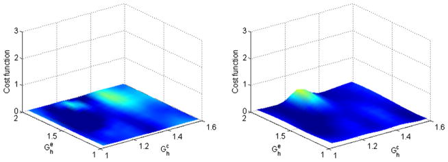
Contour of the cost function for flow reductions within the self-compensatory regime (left), γ = 1.2, ε = 0.8 and (right) γ = 1.4, ε = 0.6.

4.3. Deterministic optimization results

Example 1

The first example illustrates the application of optimization in a one-dimensional example. The goal is to find the optimal collagen pre-stretch $G_h^c$ when the pressure in the artery exceeds the homeostatic value by 50%, i.e., γ = 1.5. This optimization problem is defined as ${\widehat{G}}_h^c=argmin\mathcal{J}(G_h^c;\epsilon ,\gamma ,G_h^e,p^K,p^c)$. The range of optimization parameter values was chosen as p^K = [2.0, 20.0], $G_h^c=[1.0,1.6]$, and $G_h^e=[1.0,2.2]$. In the first example, we fixed all parameters except $G_h^c$ to their nominal values, p^K = 10.0 and $G_h^e=1.4$, and optimized for $G_h^c$.

The variation of the cost function with $G_h^c$ is shown in Fig. 7. Low pre-stretch values are unable to provide structural reinforcement to the artery, while higher pre-stretches result in the collagen fiber yielding prematurely. Over the range of loading conditions considered, we observed that the optimal deposition stretch for collagen fibers was between 1.06 and 1.1, as expected based on prior studies [13]. Next, we allowed $G_h^e$ to vary. The optimal $G_h^c$ depends on the value of $G_h^e$ (and vice versa), as observed in Fig. 8. The optima shifts to the left for the case of larger perturbations in loading because the fibers yield earlier. This finding motivates the need to perform multi-dimensional optimization.

Fig. 7.

Contour of the cost function for the one-dimensional optimization example for the prestretch of collagen for 3 different perturbations in hemodynamics.

Fig. 8.

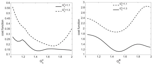
Variation of cost function corresponding to (left) ε = γ = 1.2 and (right) ε = γ = 1.4 over $G_h^e$ for two different values of $G_h^c$ . The optima as well as the curves shift due to the cross-correlating effects of the two variables.

Example 2

Here, we optimize the two pre-stretches as well as the four G&R rate parameters, defined as $(\widehat{p^G},\widehat{p^K})=argmin\mathcal{J}(p^G,p^K;\epsilon ,\gamma ,p^c)$. Motivated by the hemodynamic range that allowed self-compensatory behavior from Section 4.2.1, we choose four different combinations of insults corresponding to ε = 1.2, 1.4 and γ = 1.2, 1.4. It is not well known whether the artery in vivo differentiates between homeostatic and near-homeostatic states. Hence, in addition to computing the optimal values, we also compute the range of parameters that achieve a state within 5% of the homeostatic values.

We performed a 6 dimensional optimization over the space of p^K and p^G, with results shown in Table 2. The reduction in cost function as well as its individual terms are plotted in Fig. 9, which shows that both the wall shear stress and intramural wall stress are reduced significantly from their starting values.

Table 2.

Range of optimal parameters that maintains the artery within 5% of its homeostatic stresses and the optimal parameters that minimizes cost function for the deterministic optimization problem.

Conditions	$G_h^c$	$G_h^e$	$K_1^c$	$K_2^c$	$K_1^m$	$K_2^m$	Optimal
γ = 1.2, ε = 1.2	[1.03,1.08]	[1.70,2.2]	[2.0,2.0]	[2.0,2.0]	[2,3.8]	[2,7.4]	(1.05,2.18,2.0,2.0,2.00,2.00)
γ = 1.2, ε = 1.4	[1.03,1.12]	[1.47,1.73]	[2.0,2.0]	[2.0,2.0]	[2.15,3.8]	[2.5,7.4]	(1.10,1.70,2.0,2.0,2.14,3.17)
γ = 1.4, ε = 1.2	[1.03,1.10]	[1.20,1.70]	[2.0,2.0]	[2.0,2.0]	[2,2.83]	[2,3.8]	(1.06,1.60,2.0,2.0,2.00,2.00)
γ = 1.4, ε = 1.4	[1.04,1.11]	[1.2,2.0]	[2.0,2.0]	[2.0,2.0]	[2,2.2]	[2,3.8]	(1.08,1.44,2.0,2.0,2.00,2.00)
Intersection set	[1.04,1.08]	[1.70,1.73]	[2.0,2.0]	[2.0,2.0]	[2.0,2.2]	[2.0,3.8]	-

Fig. 9.

Evolution of individual terms in the cost function-normalized shear stress, normalized intramural stress and their total for ε = γ = 1.4.

The pre-stretch of elastin was found to be consistently higher than that of collagen. This is expected because elastin is produced primarily in the perinatal period, and is stretched over a much larger time scale¹. Results show that optimal p^K values lie near the lower boundary of the parameter space (close to 2.0), indicating that it is not mechanically favorable for the artery to arbitrarily increase the rate of collagen fiber production. Numerically, this implies that the artery does not seek to “over-correct” via extreme thickening. Because we showed earlier that very low values of p^K are not sufficient to maintain a favorable arterial response, the present results suggest that there is a mechanically optimal rate of production, given the other model parameters.

Impact of varying the range of K_c and K_m

Because the optimal values of K_c and K_m were close to the lower bound, we repeated the optimization with a lower bound of 0.1 for p^K. Two interesting phenomena were observed: (a) for the case of ε = γ (either 1.2 or 1.4), a smaller gain parameter for collagen turnover due to modified intramural stress (up to around 0.8) could compensate for a larger gain parameter for collagen turnover due to modified shear stress, and (b) for this range of inputs, some simulations resulted in unbounded nonphysical growth, such as when both K¹ and K² were smaller than 1.0. Both of the above-mentioned phenomena can be understood from Fig. 3. However, there are no gain parameters below 2.0 with a lower cost function value, thus justifying our choice of the original range.

5. Robust optimization of arterial adaptations

5.1. Stochastic optimization methods

We recently developed a stochastic SMF method with proven convergence that combines the collocation method with the deterministic SMF for robust optimization [14]. We previously demonstrated this algorithm on several constrained stochastic optimization problems, including examples of structural reliability, stochastic inverse heat conduction, concentration source identification with stochastic dispersion properties [14], and optimization of anastomosis angles in bypass grafts [20]. The algorithm performed well in both efficiency and ability to reach a known optimal solution, and showed significant improvement over traditional Monte-Carlo techniques [24].

In general, deterministic cost functions have the form (p) where p is the set of input parameters. Stochastic cost functions require an additional parameter ξ, which is a vector of stochastic parameters. The stochastic cost function is defined in general as:

$$\mathcal{J}(p,\mathit{\xi })=\sum _{i=1}^{N_c}\left({\alpha }_i\mathbf{E}({\mathcal{J}}_i(p,\mathit{\xi }))+\sum _{j=1}^{N_m}{\beta }_{ij}{\mathbf{M}}^j({\mathcal{J}}_i(p,\mathit{\xi }))\right),$$ (8)

where is the robust objective function, N_c and N_m are the number of cost functions and statistical moments respectively, and E(.) and M(.) are the expectation and moment operators respectively, with α and β the corresponding weights. The functions in Eq. (8) are individual cost functions. For example, in the case of G&R, we could employ the deviation from homeostatic stress as one cost function and time to achieve homeostasis as another, in which case N_c would be 2. The first term is the deterministic cost function if N_m = 2, the second term is the standard deviation of the solution. With an increasing number of statistical moments, the solution has an optimal combination of a small cost function and an increasingly narrow probability density. We have shown in an earlier work that the optima can be significantly affected by the inclusion of statistical moments [20].

5.1.1. Numerical coupling

SMF and adaptive sparse grid methods are both non-intrusive and flexible in their implementation. In each iteration of the optimization algorithm, the SMF method produces a set of parameters that is fed into the G&R code, and the cost function is evaluated. Robust optimization requires statistics to be computed in each cost function evaluation, and this is done with the collocation method described earlier. A schematic of the coupling is shown in Fig. 10. We have flexibility to use multiple processors to perform simulations for different input parameters at each stage of the algorithm.

Fig. 10.

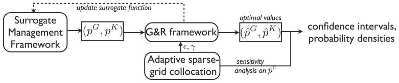
A schematic of coupling the G&R, stochastic collocation, and SMF frameworks. Input parameters to the G&R code are provided by the SMF and the collocation methods.

5.2. Robust arterial adaptation: cost function definition

For simplicity, we included only the first statistical moment (the standard deviation) in our cost function to enforce robustness. We sought an optimal value of the control parameters p^G, p^K over a range of loading conditions. We assumed that the loading conditions are stochastic over the same range of values as in the deterministic optimization problem, i.e., γ ~ [1.2, 1.4] and ε ~ [1.2, 1.4], and uniformly distributed.

The cost function was defined as a weighted sum of the mean cost and its standard deviation (i.e. N_m = 1 and N_c = 1 in Eq. (8)), hence

$${\mathcal{J}}_s={\mu }_{\mathcal{J}}+{\sigma }_{\mathcal{J}},$$

where mean and standard deviation terms are given by

$${\mu }_{\mathcal{J}}=\mathbf{E}(\mathcal{J}(p^G,p^K;\epsilon (\mathit{\xi }),\gamma (\mathit{\xi }),p^c))$$

and

$${\sigma }_{\mathcal{J}}=\sqrt{\mathbf{E}{(\mathcal{J}(p^G,p^K;\epsilon (\mathit{\xi }),\gamma (\mathit{\xi }),p^c))}^2-{\mu }_{\mathcal{J}}^2},$$

respectively. The weighting terms in Eq. (8) were chosen to be 1. This choice was motivated from our observation that the mean and standard deviation at the initialization stage were of the same magnitude (0.4 and 0.2 respectively). The stochastic collocation method was used to define the cost function as

$$\mathcal{J}(p^G,p^K;\epsilon (\mathit{\xi }),\gamma (\mathit{\xi }),p^c)=\sum _{i=1}^{N_c}\mathcal{J}(p^G,p^K;\epsilon ({\xi }_i),\gamma ({\xi }_i),p^c){\mathcal{L}}_i(\mathit{\xi }).$$

5.3. Stochastic optimization results

The stochastic SMF method converged after ~ 2000 simulations. We performed 221 cost function evaluations and for each of these evaluations, between 8 to 13 simulations to account for uncertainties. The stochastic optima insured that both the average response and its standard deviation were minimized. We found that the optimal parameter set was $(G_h^c,G_h^m,K_1^c,K_2^c,K_1^m,K_2^m)=(1.07,1.25,2.2,2.0,2.15,2.0)$.

These values are very similar to those for the deterministic optimization obtained in the previous section. This implies that the deterministic parameters maintain a near-optimal response through a wide range of loading conditions. The existence of a parameter set capable of optimality over a range of loading conditions underscores the structural integrity and robustness that a combination of elastin, collagen and SMC provide to the arterial wall. Additionally, these results show that the results of the G&R simulations are robust to perturbations in the wall properties. These simulations reveal that normal arterial wall constituents eliminate the necessity for additional structural support for modest mechanical perturbations.

6. Effect of material uncertainties in G&R predictions

To increase trust in our simulation and optimization results, we evaluated confidence intervals. Such intervals quantify the range of parameter values of interest for a given level of confidence. Given a confidence level of, say, 99%, we computed the range of outputs within which 99% of the samples would lie. To evaluate confidence intervals, we varied the relevant input (here p^c) over its range of values, computed a response surface with stochastic collocation, and evaluated the confidence intervals by constructing a histogram.

6.1. Input uncertainties

Here, we set the range of values for material parameters to be p^c ~ [μ − μ × 0.75, μ + μ × 0.75] using experimental data [36]. Since we did not know the probability density function within these bounds, we assumed different input distributions and tested robustness of results against these assumptions. For the unbounded Gaussian distribution, we insured that 99.9% of the input samples were within the given bounds, hence reliably inferring up to 99% confidence intervals. Standard deviations for the distributions were computed based on the mean values, the given input bounds, and the input distribution. The mean values of the material parameters were chosen as $c_1^i=1.4e6,c_2^i=22.0$ and $c_2^m=3.5$. Using a 6-parameter stochastic collocation method, we evaluated the sensitivity of outputs to perturbations in these material parameters.

6.2. Confidence intervals and sensitivities

We performed 849 computational simulations using the adaptive sparse grid method, compared to 3937 that would be needed with standard Smolyak sparse grid collocation (refer Table 3). Plots of sensitivity and output bounds are shown in Fig. 11, indicating that the outputs were robust. This implies that variability in material properties across patients (assuming this was the source of input variability) would not significantly affect the outcomes of the G&R simulation. This also shows that the G&R model predictions were robust to fluctuations in material properties.

Table 3.

Comparison of confidence intervals for different variables under three different input distributions.

Variable	Distribution	90%	95%	99%
Δσm	Uniform	[0.069,0.071]	[0.069,0.071]	[0.068,0.071]
Δσm	Gaussian	[0.065,0.072]	[0.065,0.073]	[0.064,0.074]
Δσm	Lognormal	[0.069,0.071]	[0.069,0.071]	[0.069,0.071]
Δσc1	Uniform	[0.083,0.121]	[0.081,0.123]	[0.074,0.128]
Δσc1	Gaussian	[0.083,0.124]	[0.080,0.126]	[0.075,0.131]
Δσc1	Lognormal	[0.086,0.123]	[0.082,0.127]	[0.076,0.130]
Δτ(×10−3)	Uniform	[3.335,3.486]	[3.323,3.494]	[3.310,3.507]
Δτ(×10−3)	Gaussian	[3.257,3.669]	[3.235,3.680]	[3.190,3.700]
Δτ(×10−3)	Lognormal	[3.349,3.514]	[3.340,3.523]	[3.312,3.528]
thomeo(days)	Uniform	[255,328]	[252,331]	[249,336]
thomeo(days)	Gaussian	[244,330]	[239,335]	[232,343]
thomeo(days)	Lognormal	[239,322]	[238,327]	[237,334]

Fig. 11.

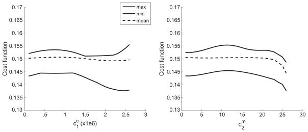
Bounds of the cost function across the parameter space plotted for (left) collagen fiber and (right) SMC.

Table 3 compares confidence intervals for the three different probability distribution functions for different quantities of interest. We insured that the values in the table were converged by performing a higher level quadrature and observed that these values changed by less than 2%. The table shows that the variability in the confidence intervals was limited to 5%, indicating that the probability distribution was not a critical input. We observed that wall shear stresses reached homeostatic values for almost all inputs. The time taken to reach within 5% of homeostasis had the maximal difference across parameters, and hence the maximum range in confidence intervals. This suggests that changing material properties results in the arteries taking different times to adapt, though the end condition was robust. Fig. 12 shows changes in the probability distribution functions for different input distribution assumptions.

Fig. 12.

Comparison of probability mass function for the number of days to achieve within 5% of homeostatic state for three different input distributions.

Parameter rankings

The sensitivities computed above assumed the G&R parameters, p^K and p^G, were optimal. Hence, we performed a 12 parameter study that varied the 6 G&R parameters in addition to p^c, i.e., the sensitivities to p^c were no longer computed at the optimal p^K and p^G. Approximately 4000 simulations were performed to achieve convergence. The PDF of the final stress state exhibited a larger variation compared to the PDF for the optimal G&R parameters. We found that the final stress state was more sensitive to p^G than to p^K. Fixing p^G at its optimal value, the computed across the range of p^c and p^K did not change significantly. However, allowing p^G to vary over its allowable range resulted in a 10-fold increase in the confidence intervals, with some simulations resulting in unbounded growth. This finding suggests that the parameters most critical to maintaining long-range homeostasis, in decreasing order, are p^G, p^K and p^c. The time taken to reach homeostasis was most sensitive to changes in p^G and p^c.

7. Discussion

We have demonstrated the utility of a scalable and modular framework for parametric sensitivity analysis and optimization of G&R model parameters. We showed that the adaptive stochastic collocation method scales almost linearly with the number of parameters, making it an attractive alternative to Monte-Carlo methods for simulation-based analysis. Further, this method is non-intrusive and hence can be used in conjunction with existing deterministic solvers. The framework is easily scalable and can be parallelized at each level of the algorithm, such that several multi-proccessor jobs can be run simultaneously.

We computed optimal wall properties and G&R parameters for a cylindrical basilar artery that restored homeostatic conditions under different altered flow and pressure conditions. Using deviation from homeostatic stress as a key term in the cost function, we showed that optimal conditions could be maintained over a reasonably broad range of loading conditions. Sensitivity of the optimal configuration to the material parameters was quantified through a stochastic collocation method. We found that the cost function was robust with respect to the material parameters p^c, meaning that different patients (with different material parameters) could reach similar stress states. We ranked parameters according to two criterion - (i) their ability to restore homeostasis, which was robust to variations in p^c and to an extent p^K, but not p^G and (ii) time to achieve homeostasis, which was robust to variations in p^K but sensitive to variations in p^c and p^G. The time to reach homeostasis varied significantly with parameter values.

The framework presented provides the first systematic application of uncertainty quantification and robust optimization tools to soft tissue growth and remodeling. As an illustrative example, we studied basilar arterial adaptations over a range of modest perturbations and observed that homeostatic conditions can be restored for this range. Although this class of problems provided a prudent starting point, the challenge facing our community is to develop similarly reliable simulations for much more complex situations, including arterial G&R in surgical planning, disease progression, responses to medical devices, and so forth. In each, there will be a need to collect longitudinal data sufficient to establish appropriate functional forms for the requisite constitutive equations and ranges of parameter values. Parameter sensitivity studies can aid the experimental design and uncertainty quantification can help establish confidence in the final predictions. Both can aid in the identification and numerical testing of competing hypotheses, which should aid further in reducing the experimental need.

There is, of course, a similar need to continue to improve our methods for parameter sensitivity analyzes and uncertainty quantification. For example, the choice of cost function remains one of the major challenges in computing optimal G&R parameters. The relative contributions of intramural stress and wall shear stress to the cost function, or the emphasis (weighting coefficient) on the importance of these stresses, can only be inferred through experiments. Toward this end, the present tools provide a framework with which to pose and test competing hypotheses for weighting functions that could then be compared against experimental data. We believe this will be an important area of future work. We also suggest that the definition of input stochastic space should be an area for future investigation, both through adding sources of uncertainties and removing dimensions where the quantity of interest is relatively flat. We suggest exploring other quadrature techniques such as sparse pseudospectral approximation methods [37] to offset numerical issues such as negative quadrature coefficients that may arise using standard quadrature.

References

- 1.Humphrey JD. Vascular adaptation and mechanical homeostasis at tissue, cellular and sub-cellular levels. Cell Biochem Biophys. 2008;50:53–78. doi: 10.1007/s12013-007-9002-3. [DOI] [PubMed] [Google Scholar]
- 2.Figueroa CA, Baek S, Taylor CA, Humphrey JD. A computational framework for fluid-solid-growth modeling in cardiovascular simulations. Comput Methods Appl Mech Engrg. 2008;198:3583–3602. doi: 10.1016/j.cma.2008.09.013. [DOI] [PMC free article] [PubMed] [Google Scholar]
- 3.Humphrey JD, Rajagopal K. A constrained mixture model for growth and remodeling of soft tissues. Math Mod Meth Appl Sci. 2002;12(3):407–430. [Google Scholar]
- 4.Kuhn E, Maas R, Himpel G, Menzel A. Computational modeling of arterial wall growth. Biomech Model Mechanobiol. 2007;6:321–331. doi: 10.1007/s10237-006-0062-x. [DOI] [PubMed] [Google Scholar]
- 5.Taber LA. A model for aortic growth based on fluid shear and fiber stresses. J Biomech Eng. 1998;120:348–354. doi: 10.1115/1.2798001. [DOI] [PubMed] [Google Scholar]
- 6.Tozeren A, Skalak R. Interaction of stress and growth in a fibrous tissue. J Theor Biol. 1988;130(3):337–350. doi: 10.1016/s0022-5193(88)80033-x. [DOI] [PubMed] [Google Scholar]
- 7.Rachev A. A model of arterial adaptation to alterations in blood flow. J Elasticity. 2000;61(1–3):83–111. [Google Scholar]
- 8.Rodriguez EK, Hoger A, McCulloch AD. Stress-dependent finite growth in soft elastic tissues. J Biomech. 1994;27(4):455–467. doi: 10.1016/0021-9290(94)90021-3. [DOI] [PubMed] [Google Scholar]
- 9.Watton PN, Hill NA, Heil M. A mathematical model for the growth of the abdominal aortic aneurysm. Biomech Model Mechanobiol. 2004;3:98–113. doi: 10.1007/s10237-004-0052-9. [DOI] [PubMed] [Google Scholar]
- 10.Kroon M, Holzapfel GA. A model for saccular cerebral aneurysm growth by collagen fiber remodeling. J Theor Biol. 2007;247:775–787. doi: 10.1016/j.jtbi.2007.03.009. [DOI] [PubMed] [Google Scholar]
- 11.Valentin A, Humphrey JD. Evaluation of fundamental hypotheses underlying constrained mixture models of arterial growth and remodeling. Phil Trans RSoc A. 2009;367:3585–3606. doi: 10.1098/rsta.2009.0113. [DOI] [PMC free article] [PubMed] [Google Scholar]
- 12.Valentin A, Cardamone L, Baek S, Humphrey JD. Complementary vasoactivity and matrix remodeling in arterial adaptations to altered flow and pressure. J R Soc Interface. 2009;6(32):293–306. doi: 10.1098/rsif.2008.0254. [DOI] [PMC free article] [PubMed] [Google Scholar]
- 13.Valentin A, Humphrey JD. Parameter sensitivity study of a constrained mixture model of arterial growth and remodeling. J Biomech Eng. 2009;131:101006-1–101006. 11. doi: 10.1115/1.3192144. [DOI] [PMC free article] [PubMed] [Google Scholar]
- 14.Sankaran S. Stochastic optimization using a sparse-grid collocation scheme. Probabilist Eng Mech. 2009;24(3):382–396. [Google Scholar]
- 15.Sankaran S, Marsden AL. A stochastic collocation method for uncertainty quantification and propagation in cardiovascular simulations. J Biomech Eng. 2011;133:031001. 1. doi: 10.1115/1.4003259. [DOI] [PubMed] [Google Scholar]
- 16.Xiu D, Hesthaven JS. High order collocation methods for the differential equation with random inputs. J Sci Comput. 2005;27:1118–1139. [Google Scholar]
- 17.Audet C, Dennis JE., Jr Mesh adaptive direct search algorithms for constrained optimization. SIAM J Optim. 2006;17(1):2–11. [Google Scholar]
- 18.Marsden AL, Feinstein JA, Taylor CA. A computational framework for derivative-free optimization of cardiovascular geometries. Comput Methods Appl Mech Engrg. 2008;197(21–24):1890–1905. [Google Scholar]
- 19.Yang W, Feinstein JA, Marsden A. Constrained optimization of an idealized y-shaped baffle for the Fontan surgery at rest and exercise. Comput Methods Appl Mech Engrg. 2010;199(33–36):2135–2149. [Google Scholar]
- 20.Sankaran S, Marsden AL. The impact of uncertainty on shape optimization of idealized bypass graft models in unsteady flow. Phys Fluids. 2010;22:121902. [Google Scholar]
- 21.Sankaran S, Audet C, Marsden AL. A method for stochastic constrained optimization using derivative-free surrogate pattern search and collocation. J Comput Phys. 2010;229(12):4664–4682. [Google Scholar]
- 22.Xiu D, Karniadakis GE. Modeling uncertainty in steady state diffusion problems via generalized polynomial chaos. Comput Methods Appl Mech Engrg. 2002;191:4927–4948. [Google Scholar]
- 23.Babuska I, Nobile F, Tempone R. A stochastic collocation method for elliptic partial differential equations with random input data. ICES report. 2005:05–47. [Google Scholar]
- 24.Metropolis N, Ulam S. The Monte-Carlo method. J Amer Statist Assoc. 1949;44(247):335–341. doi: 10.1080/01621459.1949.10483310. [DOI] [PubMed] [Google Scholar]
- 25.Najm HN. Uncertainty quantification and polynomial chaos techniques in computational fluid dynamics. Annu Rev Fluid Mech. 2009;41:35–52. [Google Scholar]
- 26.Gerstner T, Griebel M. Numerical integration using sparse grids. Numer Algorithms. 1998;18(3):209–232. [Google Scholar]
- 27.Eldred MS, Webster CG, Constantine PG. Design under uncertainty employing stochastic expansion methods. Am J Aeronaut Astronaut. 2008;2008–6001:1–22. [Google Scholar]
- 28.Klimke A. PhD Thesis. Universitt Stuttgart, Shaker Verlag; Aachen: 2006. Uncertainty modeling using fuzzy arithmetic and sparse grids. [Google Scholar]
- 29.Eldred MS. Recent advances in non-intrusive polynomial chaos and stochastic collocation methods for uncertainty analysis and design. AIAA. 2009;2009–2274:1–37. [Google Scholar]
- 30.Marsden AL, Wang M, Dennis JE, Jr, Moin P. Optimal aeroacoustic shape design using the surrogate management framework. Optim Eng. 2004;5(2):235–262. [Google Scholar]
- 31.Booker AJ, Dennis JE, Jr, Frank PD, Serafini DB, Torczon V, Trosset MW. A rigorous framework for optimization of expensive functions by surrogates. Struct Optim. 1999;17(1):1–13. [Google Scholar]
- 32.Queipo NV, Haftka RT, Shyy W, Goel T, Vaidyanathan R, Kevin Tucker P. Surrogate-based analysis and optimization. Prog Aerosp Sci. 2005;41(1):1–28. [Google Scholar]
- 33.http://www.imm.dtu.dk/hbni/dace/
- 34.Abramson MA, Audet C, Couture G, Dennis JE, Jr, Le Digabel S, Tribes C. The NOMAD project [Google Scholar]
- 35.Audet C, Dennis JE., Jr A progressive barrier approach to derivative-free nonlinear programming. SIAM J Optim. 2009;20(1):445–472. [Google Scholar]
- 36.Wagner HP, Humphrey JD. Differential passive and active biaxial mechanical behaviors of muscular and elastic arteries: basilar versus common carotid. J Biomech Eng. 2011;133:051009-01–051009-10. doi: 10.1115/1.4003873. [DOI] [PubMed] [Google Scholar]
- 37.Constantine PG, Eldred MS, Phipps ET. Sparse pseudospectral approximation method. Comput Methods Appl Mech Engrg. 2012;229(232):1–12. [Google Scholar]