

Abstract
Quantitative and qualitative loss of tropical forests prompted international policy agendas to slow down forest loss through reducing emissions from deforestation and forest degradation (REDD)+, ensuring carbon offset payments to developing countries. So far, many African countries lack reliable forest carbon data and monitoring systems as required by REDD+. In this study, we estimate the carbon stocks of a naturally forested landscape unaffected by direct human impact. We used data collected from 34 plots randomly distributed across the Mount Birougou National Park (690 km2) in southern Gabon. We used tree-level data on species, diameter, height, species-specific wood density and carbon fraction as well as site-level data on dead wood, soil and litter carbon to calculate carbon content in aboveground, belowground, dead wood, soil and litter as 146, 28, 14, 186 and 7 Mg ha−1, respectively. Results may serve as a benchmark to assess ecosystem carbon loss/gain for the Massif du Chaillu in Gabon and the Republic of Congo, provide field data for remote sensing and also may contribute to establish national monitoring systems.
Resume
Les pertes qualitatives et quantitatives de forêt tropicale ont poussé les calendriers politiques internationaux à ralentir la perte de forêts au moyen des mécanismes REDD+, qui garantissent le paiement compensatoire des émissions de carbone aux pays en développement. Jusqu'à présent, de nombreux pays africains ne disposent pas encore de données fiables sur le carbone forestier, pas plus que de systèmes de suivi exigés par les REDD+. Dans cet article, nous estimons les stocks de carbone d'un paysage de forêt naturelle non affecté par des impacts humains directs. Nous avons utilisé les données provenant de 34 parcelles réparties au hasard dans le Parc National du Mont Birougou (690 km²), dans le sud du Gabon. Nous avons utilisé trois niveaux de données pour les espèces, le diamètre, la hauteur et la densité spécifique du bois par espèce, et la fraction de carbone ainsi que des données au niveau du site sur le carbone du bois mort, du sol et de la litière pour calculer le contenu en carbone au-dessus du sol, en dessous, dans le bois mort, le sol et la litière, à savoir, respectivement, 146, 28, 14, 186 et 7 mg ha−1. Ces résultats peuvent servir de données de référence pour évaluer la perte ou le gain de carbone de l'écosystème pour le Massif du Chaillu, au Gabon, et en République du Congo, constituer des données de terrain pour la détection à distance et aussi contribuer à établir des systèmes de suivi au niveau national.
Keywords: biomass, inventory, mosaic cycle, REDD+, tropical forests
Introduction
The alarming rate of loss in quantity as well as quality of carbon-dense tropical forests has prompted international policy agendas to suggest additional carbon crediting mechanisms. The negotiations first initiated Reducing Emissions from Deforestation in Montreal, 2005 (FCCC/CP/2005/MISC 1) and expanded it to Reducing emissions from Deforestation and forest Degradation (REDD) in the Bali Action Plan (Decision 1/CP. 13). In Copenhagen (COP 15, 2009) and Cancun (COP 16, 2010), REDD was extended to REDD+ considering forest conservation, sustainable forest management and enhancement of forest carbon stocks. COP 17 (Durban, 2011) further emphasized the earlier decisions on reference emission and forest reference levels.
For implementation, the establishment of reliable national forest monitoring systems (Decision 4/CP. 15) is essential. Combinations of remote sensing- and ground-based carbon inventories are suggested to estimate anthropogenic greenhouse gas emissions and removals [Decision 4/CP. 15 Paragraph 1(d)]. According to Decision 1/CP. 16 III C, forest-related emission reductions need to be systematically measured, reported and verified including carbon stocks in five pools: (i) aboveground biomass (AGB), (ii) belowground biomass (BGB), (iii) dead wood, (iv) litter and (v) soil.
Estimates for Africa show a wide range between 76 and 231 MgC ha−1 (Brown & Lugo, 1984; Brown, Gillespie & Lugo, 1989; Brown, Gaston & Daniels, 1996; Clark et al., 2001; FAO, 2007; Ramankutty et al., 2007; Saatchi et al., 2011). One of the reasons for the uncertainty in the estimated biomass carbon of tropical forests is the lack of standard models to calculate AGB from field measurements (Chave et al., 2005). For Gabon, no validated biomass equation exists so far (Maniatis, 2010). Estimates based on basic information collected in the field [diameter at breast height (DBH), height, wood density, carbon fraction of wood, litter mass and litter carbon fraction and soil density and soil carbon fraction] are still the best means to provide reliable results.
In this work, we provide an example to calculate carbon stocks in the undisturbed forest of the Mount Birougou National Park in the Massif du Chaillu, Gabon. We thereby provide ground-truthing data for remote sensing and provide a benchmark for the potential carbon stocks of unmanaged forests located within the area of 35,000 km2 of the Massif du Chaillu.
Materials and methods
Study area
The study area was located in the vast intact block of evergreen rain forest of Monts Birougou National Park covering an area of 690 km2. Common tree species include Dacryodes macrophylla (Oliv.) H.J.Lam, Aucoumea klaineana Pierre, Centroplacus glaucinus Pierre, Coelocaryon preussi Warb., Plagiostyles africana Prain ex De Wild. Santiria trimera (Oliv.) Aubrév., Scorodophloeus zenkeri Harms and Uapaca guineensis Müll.Arg. Mean annual precipitation and temperature are 1800 mm (Maloba Makanga, 2010) and 22°C, respectively (Service de Climatologie – unpublished March 04, 2005). The rainy season extends from mid-September to June with lower and less interspersed rainfall during December and January, and the dry season lasts almost 3 months from mid-June to mid-September (Fig. 1). Soil type is Ultisol containing Kaolinite (60%), Goethite (11%), Gibbsite (8%) and 20% other minerals (Chatelin, 1968).
Figure 1.

Average monthly precipitation (mm) and mean daily temperature (°C) for the Mt. Birougou region. Data were produced by MarkSim, a stochastic weather generator for the tropics (Jones & Thornton, 1999) including the corrections for the Congo basin (Bednar, 2011)
Today, the national park is uninhabited, but in colonial times a few villages existed along a migration route crossing the eastern edge of today's park from north to south. Among these villages, only one (i.e. Kuendji – situated on a hilltop aside the headwater of the Lolo river) was located inside the park and was given up before 1900 (Ilembi Makinda Léon-Paul 2005, personal communication, March 14). For sampling, we excluded a buffer zone of 3 km along the migration route.
Data
Thirty-four sampling plots (fifteen in August 2004 and nineteen in March 2005) were randomly selected across the forest. In this study, we applied the point sampling inventory method (Bitterlich, 1948; Avery & Burkhart, 1983) using a gauge with a 2-cm-wide opening plate and a 65-cm-long string. Basal area factor (BAF) of the instrument was calculated as 2.37 m2 ha−1 (Eq. 1) and corrected for slope (BAFcor), if necessary (Eq. 2).
| (1) |
| (2) |
Where w is opening width of instrument (cm) and R is distance between eye and opening gauge (cm), and cos (α) is cosine of slope angle.
For each tallied tree, the tree species, the orientation and distance from the plot centre, DBH and tree height were recorded with diameter tape and Vertex III hypsometer (Haglöf, Sweden), respectively. Herbarium samples of 37 tree species were taken to the ‘Herbier National du Gabon’ for species verification. If buttress or stilt roots were present at 1.3 m, diameter was measured immediately above the buttresses or stilt roots. Basal area of a tree (BAtree), number of representative trees per hectare (Nrep), tree volume (Volumetree) and total volume (Volumetotal) were calculated according to Eqs. 3–6. An average form factor (FF) of 0.6 (Cannell, 1984) was used.
| (3) |
| (4) |
| (5) |
| (6) |
In point sampling, each tallied tree represents a specific virtual nested circular plot area with borderline radius Rplot.(Eq. 3)
| (7) |
The mean of the virtual areas of all tallied trees gives virtual plot size, for our 34 plots ranging from 212 to 1227 m2 with a mean of 610 m2.
One to three stem cores were recovered from 55 species until the corer broke in a stem of Swartzia fistuloides Harms. Cores were oven dried for 24 h at 105°C, and part of each sample was sent to the University of Vienna for carbon fraction determination. For trees with no values, we used the weighted mean derived from the trees with assigned values. For wood density determination, cores collected from 43 species were equilibrated (4°C, 12% relative humidity) for constant weight, separated into 5–18 subsamples and each of which was analysed for density using the submerge method. Wood density for trees not cored was taken from literature [Dahms, 1999; Société National des Bois du Gabon – unpublished September 9, 2004; Wood Density Database, 2009 http://www.worldagroforestry.org/sea/products/AFDbases/WD/Index.htm (accessed on September 4–October 30, 2009)] ranging from 400 kg m−3 (Funtumia africana Stapf) to 1200 kg m−3 (Afzelia bipindensis Harms). For trees with no values, we assigned the weighted mean density (WDavg, Eq. 8). Specific wood density (WD0%) of corresponding tree species was calculated (Eq. 9, Kollman & Cote, 1968).
 |
(8) |
| (9) |
Where Ni is the number of trees in ith tree species, ρi is the wood density of ith tree species, WDmc is the wood density (kg m−3) at moisture content (mc%), mc is the moisture content in wood while measuring wood density, and VS is the volumetric shrinkage of the tree species taken from Dahms (1999).
Considering the heterogeneity and species diversity in the tropics, the biomass of each tree recorded in the plot was calculated using the corresponding tree-specific measurement. AGB of each tree was obtained by multiplying tree volume with respective WD0%. AGB of each tree within the plots were summed to obtain AGB density in the corresponding plot. BGB was estimated from AGB using the relationship derived for the tropics by Cairns et al. (1997):
| (10) |
Aboveground carbon content of each tree was derived by multiplying tree biomass with the corresponding wood carbon fraction. For trees with no observation, we used the mean of all observed data weighted for individual abundance within all 34 plots. AGB carbon of each tree was summed to obtain AGB carbon density at the plot level. BGB carbon content was derived from AGB carbon content using Eq. 10.
Dead wood includes tallied standing dead trees, and dead and down trees if and only if the distance from the plot centre to the re-erected tree fell within the border line radius of the tree (Rplot, Eq. 7). With this criterion, dead wood observations were only made on 18 of 34 plots. Dead wood volume was calculated as given in Eqs. 3–6 and converted to dead wood biomass and dead wood carbon using the weighted averages of WD0% and carbon fraction.
Soil consisted two layers: humus rich top soil and a clayey lower soil layer with a maximum depth of 11 m observed on an eroded bank of Makanga River. Soil profiles were taken in 2005 in three replicates per plot using a single gauge soil auger made for collecting soil profiles up to 1 m depth. The high water content of the soil (sampling was during the rainy season) and the clayey soil texture resulted in a mixture zone between top and lower soil within the collected soil profile. Two soil samples were collected from each profile: One in the middle of the top soil layer and one at 0.5 m soil depth or 0.1 m below the mixture zone of top and lower soil layer if the mixture zone reached below 0.48 m soil depth, resulting in an average sampling depth for top and lower soil of 0.1 and 0.54 m. Soil density was determined from two samples collected with a soil sample ring with 8 cm diameter and 5 cm height.
Few soil samples were treated with hydrochloric acid to test the presence of CaCO3, but no evidence of it was found in any samples. The soil samples were oven dried at 105°C for 24 h, and weight of both samples was recorded before further processing. The soil samples were sieved with 2-mm sieve and roots and wooden parts removed, if present. Next samples were milled with a mixer mill (Retsch MM 200), and carbon content was determined at the University of Vienna, Austria.
Soil carbon content (SC) in the top soil layer and up to 1 m soil depth in Mg ha−1 was calculated according to Eqs. 11 and 12.
| (11) |
| (12) |
Where ρs is soil density in kg m−3, C%ts is carbon per cent in top soil, C%ls is carbon per cent in the lower soil layer and Dts is depth of top soil layer in m, measured as the distance from the soil surface to the beginning of the mixture zone to avoid overestimation from profile collection artefacts, that is, the mixture of top and lower soil layers within the soil auger.
In the case of litter, on each of the 34 plots three litter samples were randomly collected from a soil surface of 50.26 cm2 using the same sample ring. The three samples collected per plot were mixed before analyses. Samples were oven dried at 105°C for 24 h, weighed, milled and analysed for carbon content as described for soil samples.
Results
Floristic composition
On the 34 sampling plots, 85% of tallied trees were taxonomically identified to 91 species. Of these, 34 species were abundant with a single tree and eighteen with two trees, while seven of the species contributed more than 57% to the total stem number. The plant identification rates varied from 31% to 100% of the trees in each plot, with only two plots exhibiting an identification rate of <75% (Fig. 2). Among the trees identified, Caesalpiniaceae was the most diversified family with eleven tree species, followed by Annonaceae and Burseraceae with seven tree species. Burseraceae, Caesalpiniaceae and Euphorbiaceae were the three most common tree families holding 23%, 10% and 8% of total basal area (Table 1) in the forest, respectively. Of 36 recorded families, six families were only represented by a single tree (Table 1), and together, their contribution to basal area was 1.4%. By tree number, Dacryodes macrophylla (Oliv.) H.J.Lam was the most abundant tree species (approximately 10%). By diameter and height, Aucoumea klaineana Pierre (Buraseraceae), Afzelia bipindensis Harms (Caesalpiniaceae) and Erythrophleum ivorense A.Chev. (Caesalpiniaceae) were the biggest three trees.
Figure 2.
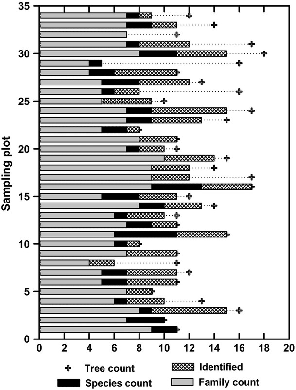
Number of trees per plot, number of trees per plot identified at the species level, number of identified species per plot and corresponding number of tree families per plot
Table 1.
Summary of species count (SC), tree count (TC), diameter at breast height (DBH, cm) and total tree height (m) by family
| Family | SC | TC | DBH | Height |
|---|---|---|---|---|
| Caesalpiniaceae | 12 | 44 (10.05) | 40.2 (9.9–129.5) | 22.8 (8.0–40.0) |
| Annonaceae | 7 | 20 (4.57) | 31.2 (5.4–63.3) | 22.0 (6.0–40.0) |
| Burseraceae | 7 | 100 (22.83) | 41.1 (3.8–135.3) | 23.1 (8.5–43.0) |
| Apocynaceae | 5 | 8 (1.83) | 21.6 (6.9–41.0) | 14.6 (7.5–26.5) |
| Olacaceae | 5 | 16 (3.65) | 44.0 (8.3–85.3) | 25.5 (11.9–35.0) |
| Mimosaceae | 4 | 15 (3.42) | 54.8 (5.6–90.4) | 28.1 (10.4–40.0) |
| Sapindaceae | 4 | 4 (0.91) | 19.0 (4.3–38.0) | 16.6 (4.5–23.2) |
| Anacardiaceae | 3 | 4 (0.91) | 20.0 (4.1–33.7) | 13.9 (9.0–20.5) |
| Euphorbiaceae | 3 | 34 (7.76) | 39.9 (4.1–82.0) | 23.7 (8.5–37.0) |
| Meliaceae | 3 | 8 (1.83) | 40.2 (5.5–93.3) | 22.4 (6.0–35.1) |
| Moraceae | 3 | 5 (1.14) | 16.1 (8.6–20.7) | 13.2 (8.6–20.0) |
| Papilionaceae | 3 | 9 (2.05) | 43.2 (9.2–116.2) | 24.3 (13.0–40.0) |
| Rubiaceae | 3 | 10 (2.28) | 20.6 (8.0–39.5) | 16.8 (8.0–31.0) |
| Rutaceae | 3 | 8 (1.83) | 44.9 (9.5–84.4) | 23.8 (14.5–33.5) |
| Guttiferae | 2 | 6 (1.37) | 26.0 (16.0–38.8) | 19.5 (15.0–24.0) |
| Myristicaceae | 2 | 21 (4.79) | 43.5 (17.5–84.0) | 25.3 (15.5–37.0) |
| Myrtaceae | 2 | 2 (0.46) | 37.1 (7.3–66.8) | 19.5 (7.5–31.5) |
| Sapotaceae | 2 | 4 (0.91) | 48.6 (40.0–68.4) | 25.2 (7.4–33.0) |
| Anisophylleaceae | 1 | 5 (1.14) | 38.9 (16.1–76.4) | 24.6 (17.0–31.0) |
| Chrysobalanacaceae | 1 | 3 (0.68) | 36.1 (26.2–47.0) | 20.9 (17.4–26.1) |
| Clusiaceae | 1 | 8 (1.83) | 38.6 (7.2–71.3) | 22.0 (8.0–31.0) |
| Ebenaceae | 1 | 2 (0.46) | 37.1 (16.2–58.0) | 20.2 (13.6–26.7) |
| Erythroxylaceae | 1 | 4 (0.91) | 20.2 (16.6–24.2) | 21.8 (19.5–25.0) |
| Fabaceae | 1 | 1 (0.23) | 46.0 | 21.3 |
| Flacourtiaceae | 1 | 1 (0.23) | 4.2 | 4.8 |
| Irvingiaceae | 1 | 2 (0.46) | 12.8 (9.9–15.7) | 14.1 (11.6–16.5) |
| Lamiaceae | 1 | 3 (0.68) | 19.2 (12.4–22.9) | 17.8 (15.0–21.0) |
| Lecythidaceae | 1 | 8 (1.83) | 51.3 (22.9–68.0) | 25.9 (18.0–39.0) |
| Loganiaceae | 1 | 1 (0.23) | 29.9 | 24.5 |
| Pandaceae | 1 | 5 (1.14) | 17.8 (10.5–26.1) | 18.9 (11.0–25.0) |
| Rhizophoraceae | 1 | 2 (0.46) | 19.3 (4.5–34.0) | 11.7 (4.0–19.3) |
| Simaroubaceae | 1 | 3 (0.68) | 59.8 (29.2–89.1) | 26.2 (15.2–34.0) |
| Steruliaceae | 1 | 1 (0.23) | 31.0 | 11.2 |
| Tiliaceae | 1 | 1 (0.23) | 26.0 | 21.1 |
| Ulmaceae | 1 | 1 (0.23) | 39.8 | 33.0 |
| Violaceae | 1 | 3 (0.68) | 22.4 (19.1–25.8) | 15.3 (12.0–19.0) |
| Unidentified | 66 (15.07) | 33.7 (6.9–75.1) | 21.2 (2.8–41.0) | |
| Total | 91 | 438 |
Values in parenthesis give the per cent of the corresponding family's representation for TC and the range of measurements for DBH and Height.
Tree-level data
The tree-level information was developed from species, DBH, total tree height and corresponding WD0% of trees in 34 plots (Fig. 2). Diameters ranged from 4.1 to 135 cm and heights from 2.8 to 43 m (Table 1).
Stem cores of 54 tree species exhibited wood carbon contents of 45.14–53.05% with a mean of 47.95% (Table 2). For trees without observed wood carbon fractions, weighted mean carbon of 48.27% was assumed.
Table 2.
Species-specific wood carbon fraction (C, %) and specific wood density (WD0%) derived from measurements using Eq. 9
| Family | Species | Local name | C (%) | WD0% |
|---|---|---|---|---|
| Anacardiaceae | Sorindeia oxyandra Bourobou & Breteler | Tsaghessa | 47.46 | 653 |
| Anacardiaceae | Sorindeia Thouars | Mutoumbu | 48.28 | 737 |
| Anacardiaceae | Trichoscypha acuminata Engl. | Amvut/Mulili | 47.85 | 729 |
| Anisophylleaceae | Poga oleosa Pierre | Ovoga | 50.88 | |
| Annonaceae | Aneulophus africanus Benth. | Mubamba | 47.78 | 691 |
| Annonaceae | Cleistopholis patens Engl. & Diels | Mukundzu | 47.50 | 641 |
| Annonaceae | Enantia letestui LeThomas | Moambe | 48.97 | |
| Annonaceae | Greenwayodendron sauveolens Verdc. | Otunga | 49.20 | |
| Annonaceae | Isolona zenkeri Engl. & Diels | Isolona | 52.19 | |
| Annonaceae | Xylopia aethiopica A. Rich | Okala | 48.93 | 715 |
| Apocynaceae | Alstonia congensis Engl. | Ekuk/Mukuku | 49.14 | 641 |
| Apocynaceae | Picralima nitida Th. & H. Dur. | Ghundu | 49.08 | 938 |
| Burseraceae | Aucoumea klaineana Pierre | Okoume | 48.41 | 467 |
| Burseraceae | Canarium schweinfurthii Engl. | Mumbili | 46.67 | 541 |
| Burseraceae | Dacryodes buettneri (Engl.) H.J.Lam | Ozigo | 47.95 | 789 |
| Burseraceae | Dacryodes klaineana (Pierre) H.J.Lam | Adjouba | 48.88 | |
| Burseraceae | Dacryodes macrophylla (Oliv.) H.J.Lam | Atom | 47.19 | 764 |
| Caesalpiniaceae | Amphimas ferrugineus Pierre ex Harms | Ikodiakodi | 48.77 | 980 |
| Caesalpiniaceae | Bikinia letestui (Pellegr.) Wieringa | Mudungu | 48.76 | 836 |
| Caesalpiniaceae | Diallum pachyphyllum Harms | Eyoum | 47.27 | |
| Caesalpiniaceae | Scorodophloeus zenkeri Harms | Divida | 48.16 | 894 |
| Caesalpiniaceae | Swartzia fistuloides Harms | Pao Rosa | 790 | |
| Caesalpiniaceae | Tessmannia africana Harms | Nkagha | 53.05 | |
| Chrysobalanaceae | Magnistipula tessmanii (Engl.) Prance | Efot | 50.43 | |
| Clusiaceae | Allanblackia Oliv. | Nsangom | 47.19 | 802 |
| Clusiaceae | Garcinia kola Heckel | Mubodi | 47.28 | 800 |
| Ebenaceae | Diospyros L. | Envila | 45.14 | |
| Euphorbiaceae | Plagiostyles africana Prain ex De Wild. | Boulou/Essoula | 45.99 | 726 |
| Euphorbiaceae | Uapaca guineensis Müll Arg. | Rikio/Bodjahambe | 52.79 | |
| Lamiaceae | Vitex L. | Ipate | 47.61 | 456 |
| Lecythidaceae | Petersianthus macrocarpus (P Beauv.) Liben | Essia | 49.98 | |
| Loganiaceae | Anthocleista vogelii Planch. | Ayinbe | 47.87 | 463 |
| Meliaceae | Carapa procera D.C. | Crabwood | 48.39 | 805 |
| Mimosaceae | Albizia Durazz. | Tsele | 48.22 | 646 |
| Moraceae | Chlorophora excelsa Benth. & Hook.f. | Mbonga | 47.82 | 603 |
| Myristicaceae | Pycnanthus angolensis (Welw.) Exell | Ilomba | 45.93 | 499 |
| Myriticaceae | Coelocaryon preussi Warb. | Ekoune/Lombe | 46.22 | 550 |
| Myriticaceae | Syzygium staudtii (Engl.) Mildbr. | Szygium | 48.38 | 781 |
| Olacaceae | Engomegoma gordonii Breteler | Engomegoma | 49.92 | |
| Olacaceae | Heisteria parviflia Sm. | Nsonso | 47.42 | 646 |
| Olacaceae | Ongokea gore Pierree | Mungueke | 47.29 | 855 |
| Olacaceae | Strombosiopsis tetrandra Engl. | Vendi | 47.41 | 881 |
| Pandaceae | Centroplacus glaucinus Pierre | Mbesse | 48.51 | 837 |
| Rubiaceae | Corynanthe mayumbensis (R.D. Good) N. Hallé ‘eH. | Mussuli | 49.16 | 915 |
| Rutaceae | Zanthoxylum heitzii (A.& P.) P.G.W. | Olon | 48.20 | 557 |
| Rutaceae | Zanthoxylum tessmannii (Engl.) A. | Bong | 48.14 | 1051 |
| Sapindaceae | Ganophyllum giganteum (A.Chev.) Hauman | Bilinga | 49.67 | 707 |
| Simaroubaceae | Odyendea gabonensis Pierre | Bundjeghe | 48.31 | 461 |
| Violaceae | Rinorea Aubl. | Issoka | 48.35 | 553 |
| Bukulu | 47.68 | 692 | ||
| Mbanza | 47.97 | 963 | ||
| Mololongo | 48.50 | 713 | ||
| Ndombela | 46.76 | 628 | ||
| Pula Tsulbatseki | 47.40 | 975 | ||
| Tombdika | 47.17 | 827 |
Wood density analysis of stem cores from 43 species revealed WD0% of 456–1051 kg m−3 with a mean of 726 kg m−3 (Table 2) close to the average 690 kg m−3 reported for 268 tropical tree species (Fearnside, 1997). Measured wood densities of 49% of species and literature values for another 26% species resulted in an average weighted WD0% of 680 kg m−3 for the remaining 25%.
For diameter–height relationship, a logarithmic DBH versus height model (Fig. 3) was fitted, explaining two-thirds of height variation by diameter (r2 = 0.67), excluding broken top trees (1.6%).
Figure 3.

Diameter versus height for 438 measured trees (open and closed symbols). Seven trees with a broken top (closed symbols) were excluded when fitting the diameter versus height model of Brown, Gillespie & Lugo (1989), resulting in regression coefficients of a = −12.0613 and b = 10.0121. Shown are the regression line (solid) and the 95% prediction interval (dashed)
Stand-level data
Because of the diversified species composition, the analyses of species-specific tree volume, biomass and carbon content for each plot was omitted. Stand-level information on these variables revealed Burseraceae, Caesalpiniaceae and Euphorbiaceae as holding 23%, 11% and 8% of total AGB of 302 Mg ha−1, respectively, and 16% attributable to unidentified trees (Table 3). Most families exhibited the highest percentage of AGB within the diameter classes from 20 to 50 cm (Table 3), which contributed 56% to total biomass (Table 4). The highest shares of basal area (21%), tree volume (21%), AGB (22%) and AGB carbon (22%) were found within 30–40 cm (Table 4). In this diameter class, tree height was 22.6 ± 4.5 m, which was 35% lower than the highest mean height by diameter class (Table 4).
Table 3.
Mean distribution of biomass (in per cent, except the first column) at family level by diameter classes
| Family | TB | 1 | 2 | 3 | 4 | 5 | 6 | 7 | 8 | 9 | 10 | 11 |
|---|---|---|---|---|---|---|---|---|---|---|---|---|
| Burseraceae | 69.6 | 1.4 | 6.5 | 13.2 | 32.0 | 21.7 | 12.1 | 4.9 | 1.0 | 2.9 | 2.1 | 2.3 |
| Caesalpiniaceae | 35.1 | 1.3 | 4.8 | 26.7 | 23.1 | 11.0 | 9.4 | 9.5 | 3.6 | 4.0 | 6.7 | |
| Euphorbiaceae | 21.8 | 4.5 | 6.1 | 18.3 | 19.1 | 12.4 | 22.0 | 6.1 | 8.0 | 3.6 | ||
| Olacaceae | 15.0 | 2.9 | 5.0 | 14.1 | 12.2 | 8.5 | 19.8 | 23.7 | 7.2 | 6.7 | ||
| Mimosaceae | 13.4 | 1.8 | 3.5 | 19.6 | 34.9 | 10.4 | 17.9 | 11.7 | ||||
| Myristicaceae | 12.8 | 3.5 | 12.2 | 21.7 | 23.2 | 21.9 | 5.6 | 6.5 | 5.5 | |||
| Annonaceae | 12.0 | 6.7 | 4.8 | 14.6 | 24.7 | 23.8 | 16.6 | 8.8 | ||||
| Lecythidaceae | 6.7 | 9.8 | 10.6 | 9.1 | 12.2 | 58.4 | ||||||
| Clusiaceae | 6.6 | 10.2 | 15.4 | 42.7 | 16.7 | 15.0 | ||||||
| Meliaceae | 6.1 | 3.3 | 10.9 | 21.1 | 15.0 | 16.8 | 14.6 | 18.3 | ||||
| Papilionaceae | 6.0 | 10.8 | 7.7 | 19.1 | 21.4 | 13.1 | 15.9 | 12.1 | ||||
| Rutaceae | 5.3 | 8.5 | 32.2 | 9.4 | 10.4 | 10.6 | 14.8 | 14.1 | ||||
| Rubiaceae | 4.9 | 17.8 | 24.6 | 11.6 | 46.0 | |||||||
| Pandaceae | 3.9 | 46.7 | 53.3 | |||||||||
| Apocynaceae | 3.8 | 11.7 | 34.6 | 48.8 | 4.9 | |||||||
| Guttiferae | 3.5 | 11.8 | 60.4 | 27.8 | ||||||||
| Erythroxylaceae | 3.2 | 51.0 | 24.1 | 24.9 | ||||||||
| Sapotaceae | 2.8 | 71.7 | 28.3 | |||||||||
| Anisophylleaceae | 2.7 | 11.4 | 17.0 | 39.0 | 32.7 | |||||||
| Sapindaceae | 2.7 | 3.6 | 27.5 | 68.9 | ||||||||
| Moraceae | 2.4 | 12.8 | 13.2 | 50.3 | 23.7 | |||||||
| Chrysobalanaceae | 1.9 | 30.8 | 30.5 | 38.7 | ||||||||
| Anacardiaceae | 1.7 | 12.4 | 21.0 | 23.5 | 43.1 | |||||||
| Simaroubaceae | 1.7 | 19.9 | 39.9 | 40.2 | ||||||||
| Ebenaceae | 1.2 | 36.6 | 63.4 | |||||||||
| Myrtaceae | 1.2 | 20.9 | 79.1 | |||||||||
| Violaceae | 1.0 | 26.5 | 73.5 | |||||||||
| Lamiaceae | 1.0 | 38.8 | 61.2 | |||||||||
| Ulmaceae | 1.0 | 100.0 | ||||||||||
| Irvingiaceae | 0.9 | 41.3 | 58.7 | |||||||||
| Tiliaceae | 0.8 | 100.0 | ||||||||||
| Rhizophoraceae | 0.7 | 15.3 | 84.7 | |||||||||
| Fabaceae | 0.6 | 100.0 | ||||||||||
| Loganiaceae | 0.6 | 100.0 | ||||||||||
| Sterculiaceae | 0.2 | 100.0 | ||||||||||
| Flacourtiaceae | 0.1 | 100.0 | ||||||||||
| Unidentified | 47.0 | 1.7 | 13.3 | 24.3 | 17.6 | 12.5 | 8.3 | 4.3 |
The columned name with tree biomass (TB, in Mg ha−1) gives the total amount for the corresponding family. In the table, 1 represents diameter class with diameter at breast height <10 cm, and 2, 3,4,5,6,7,8,9 and 10 represent diameter class of 10 cm–100 cm at 10-cm interval, respectively, and the last eleven represents for diameter class with larger than 100 cm.
Table 4.
Number of observation (Obs.), total tree height (m), basal area (BA, m2 ha−1), tree volume (TV, m3 ha−1), aboveground biomass (AGB, Mg ha−1) and aboveground biomass carbon (AGBC, Mg ha−1) by 10 cm diameter classes
| Dbh | Obs | Height | BA | TV | AGB | AGBC |
|---|---|---|---|---|---|---|
| <10 | 32 | 9.9 (2.8–29.0) | 2.45 | 15 | 9.4 | 4.6 |
| 10–20 | 54 | 15.7 (8.0–26.0) | 4.07 | 38 | 26.4 | 12.7 |
| 20–30 | 91 | 19.3 (9.0–35.0) | 6.95 | 81 | 56.0 | 27.0 |
| 30–40 | 93 | 22.6 (10.4–33.0) | 6.99 | 95 | 66.9 | 32.2 |
| 40–50 | 59 | 25.6 (7.4–40.0) | 4.42 | 68 | 47.2 | 22.7 |
| 50–60 | 49 | 27.8 (5.5–41.0) | 3.73 | 63 | 40.4 | 19.6 |
| 60–70 | 28 | 29.6 (16.0–39.0) | 2.27 | 40 | 25.8 | 12.5 |
| 70–80 | 12 | 32.8 (28.0–40.0) | 0.89 | 17 | 11.3 | 5.5 |
| 80–90 | 11 | 33.4 (28.0–40.0) | 0.79 | 16 | 9.7 | 4.7 |
| 90–100 | 4 | 35.1 (32.0–36.5) | 0.31 | 6 | 4.2 | 2.0 |
| >100 | 5 | 34.5 (25.1–43.0) | 0.36 | 7 | 4.7 | 2.2 |
| Total | 438 | 33.23 | 447 | 302.0 | 145.8 |
Without considering tree species and family, plot-level means were given as follows: Lorey's height, 27 ± 4 m; volume, 447 ± 171 m3 ha−1; AGB, 302 ± 122 Mg ha−1; and AGB carbon, 146 ± 58 Mg ha−1 (Table 5). Average BGB and carbon were estimated as 53 ± 19 and 28 ± 10 Mg ha−1, respectively and average dead wood volume, biomass and carbon were 44 ± 20 m3 ha−1, 29 ± 14 Mg ha−1 and 14 ± 7 Mg ha−1, respectively (Table 5).
Table 5.
Lorey's height (H, m), basal area (BA, m2 ha−1), tree volume (TV, m3 ha−1), biomass in aboveground (AGB, Mg ha−1), belowground (BGB, Mg ha−1) and dead wood (DWB, Mg ha−1), carbon content in aboveground biomass (AGC, Mg ha−1), belowground biomass (BGC, Mg ha−1), dead wood (DWC, Mg ha−1), top soil layer (SC-TL, Mg ha−1), soil up to 1 m (SC-1 m, Mg ha−1) and litter carbon (LC, Mg ha−1) in 34 sampling plots
| Plot | H | BA | TV | AGB | BGB | DWB | AGC | BGCCC | DWC | SC-TL | SC-1 m | LC |
| 1 | 23 | 26.52 | 338 | 213 | 40 | 43 | 103.5 | 20.9 | 20.9 | 4.4 | ||
| 2 | 27 | 23.87 | 314 | 201 | 38 | 24 | 97.1 | 19.8 | 11.6 | 2.0 | ||
| 3 | 26 | 51.78 | 713 | 461 | 78 | 221.4 | 41.0 | 1.8 | ||||
| 4 | 22 | 35.53 | 391 | 263 | 48 | 23 | 128.6 | 25.3 | 11.1 | 2.5 | ||
| 5 | 21 | 22.97 | 231 | 145 | 28 | 71.1 | 15.0 | 2.9 | ||||
| 6 | 29 | 26.04 | 359 | 215 | 40 | 103.4 | 20.9 | 3.6 | ||||
| 7 | 20 | 30.23 | 313 | 199 | 37 | 20 | 95.2 | 19.4 | 9.7 | 1.8 | ||
| 8 | 21 | 26.04 | 294 | 199 | 37 | 23 | 95.9 | 19.6 | 10.9 | 1.2 | ||
| 9 | 28 | 27.89 | 409 | 249 | 45 | 30 | 125.7 | 24.8 | 14.3 | 2.7 | ||
| 10 | 21 | 20.28 | 174 | 104 | 21 | 28 | 50.0 | 11.0 | 13.3 | 6.0 | ||
| 11 | 23 | 41.00 | 469 | 297 | 53 | 49 | 144.1 | 28.0 | 23.7 | 1.7 | ||
| 12 | 27 | 26.04 | 321 | 211 | 39 | 8 | 102.5 | 20.8 | 3.7 | 3.5 | ||
| 13 | 23 | 31.04 | 356 | 225 | 42 | 108.8 | 21.9 | 2.5 | ||||
| 14 | 22 | 37.89 | 438 | 303 | 54 | 45 | 149.0 | 28.9 | 21.5 | 2.9 | ||
| 15 | 19 | 29.70 | 294 | 196 | 37 | 93.3 | 19.1 | 1.8 | ||||
| 16 | 31 | 51.06 | 697 | 453 | 77 | 218.0 | 40.4 | 74.6 (16) | 225.6 | 9.3 | ||
| 17 | 32 | 40.86 | 679 | 463 | 79 | 221.8 | 41.0 | 67.3 (16) | 250.2 | 13.1 | ||
| 18 | 28 | 34.01 | 517 | 424 | 73 | 16 | 201.8 | 37.7 | 7.5 | 88.2 (22) | 205.0 | 11.7 |
| 19 | 31 | 36.93 | 560 | 387 | 67 | 186.5 | 35.2 | 46.1 (16) | 146.3 | 8.2 | ||
| 20 | 29 | 26.04 | 349 | 209 | 39 | 28 | 103.5 | 20.9 | 13.3 | 44.2 (17) | 159.8 | 6.9 |
| 21 | 29 | 26.18 | 431 | 300 | 54 | 145.1 | 28.2 | 56.0 (18) | 171.2 | 7.9 | ||
| 22 | 21 | 19.04 | 212 | 146 | 28 | 26 | 71.3 | 15.0 | 12.5 | 91.0 (25) | 172.4 | 9.4 |
| 23 | 35 | 36.59 | 600 | 442 | 75 | 213.3 | 39.6 | 57.4 (20) | 182.2 | 6.1 | ||
| 24 | 26 | 40.24 | 506 | 344 | 61 | 62 | 163.4 | 31.3 | 29.7 | 49.6 (18) | 186.3 | 9.9 |
| 25 | 24 | 23.67 | 234 | 179 | 34 | 17 | 85.2 | 17.6 | 8.3 | 38.0 (16) | 128.8 | 8.2 |
| 26 | 32 | 41.14 | 595 | 407 | 70 | 194.3 | 36.5 | 33.5 (13) | 167.6 | 3.7 | ||
| 27 | 33 | 31.71 | 476 | 304 | 54 | 13 | 146.4 | 28.4 | 6.5 | 59.4 (23) | 166.2 | 16.1 |
| 28 | 28 | 26.62 | 412 | 276 | 50 | 135.5 | 26.6 | 80.9 (24) | 176.4 | 11.3 | ||
| 29 | 27 | 47.42 | 719 | 512 | 86 | 247.7 | 45.2 | 69.0 (24) | 173.1 | 7.1 | ||
| 30 | 31 | 54.06 | 868 | 558 | 93 | 28 | 269.7 | 48.8 | 13.4 | 60.8 (21) | 140.2 | 12.5 |
| 31 | 27 | 47.45 | 706 | 517 | 87 | 36 | 248.6 | 45.4 | 17.5 | 54.4 (18) | 186.1 | 11.3 |
| 32 | 26 | 26.07 | 342 | 236 | 43 | 113.9 | 22.8 | 99.9 (29) | 164.4 | 21.3 | ||
| 33 | 36 | 34.78 | 531 | 388 | 67 | 187.4 | 35.3 | 97.5 (22) | 286.3 | 12.0 | ||
| 34 | 21 | 29.15 | 336 | 240 | 44 | 115.1 | 23.0 | 83.8 (17) | 248.3 | 10.1 | ||
| Avg | 27 | 33.23 | 447 | 302 | 53 | 29 | 145.8 | 28.1 | 13.9 | 65.9 (20) | 186.1 | 7.0 |
| SD | 4 | 9.39 | 171 | 122 | 19 | 14 | 58.3 | 10.0 | 6.6 | 20.1 (4) | 40.5 | 4.8 |
| Max | 36 | 54.06 | 868 | 558 | 93 | 62 | 269.7 | 48.8 | 29.7 | 99.9 (29) | 286.3 | 21.3 |
| Min | 19 | 19.04 | 174 | 104 | 21 | 8 | 50.0 | 11.0 | 3.7 | 33.5 (13) | 128.8 | 1.2 |
Values in the parenthesis give top-layer thickness in cm. SD gives one standard deviation for corresponding values.
Figure 4 shows that the carbon fraction in top soil (3.21 ± 0.81%) was significantly higher (paired t-test: t = 12.46, P < 0.001, df = 18) than in the lower soil layer (1.38 ± 0.37%). Top soil exhibited an average thickness of 20 cm (16–29 cm) holding a total of 66 ± 20 Mg ha−1 carbon. Including the lower soil up to 1 m depth resulted in a total soil carbon content of 186 ± 41 Mg ha−1(Table 5). None of the soil samples from our plots exhibited traces of charcoal or other indicators of human habitation, clearance or cultivation (Willis, Gilson & Brncic, 2004).
Figure 4.

Carbon content (% of weight of soil) in top – solid circle and lower soil – open circle in nineteen plots, resulted from the averaged of three replication, in the year 2005. The mean sampling depth for top and lower soil samples were 10 and 54 cm, respectively
Litter samples collected in August 2004 exhibited a mass of 14.1 ± 6.0 Mg ha−1, a mean carbon fraction of 40 ± 5% and a corresponding total litter carbon stock of 2.8 ± 1.3 Mg ha−1. Samples collected in March 2005 exhibited a mass of 27.5 ± 9.5 Mg ha−1, a carbon fraction 35 ± 6% and a litter carbon stock of 10.3 ± 3.0 Mg ha−1. Samples from August 2004 exhibited a significantly higher carbon fraction (t-test: t = 2.31; P = 0.02; df = 32) but a highly significant lower mass (t-test: t = −4.76; P < 0.001; df = 32) resulting in highly significant lower litter carbon stocks (t-test: t = −7.21; P < 0.001; df = 32), as compared to samples from March 2005 (Fig. 5).
Figure 5.

Litter mass, carbon fraction and total litter carbon content of samples collected in August 2004 (white boxes) and March 2005 (grey boxes). Boxes cover the data range from the 25th to the 75th percentile, the line in the box gives the median and the whiskers indicate the 10th and 90th percentiles, respectively
Discussion
Compared to other regions in Gabon, where pioneer species like Aucoumea klaineana Pierre account for 30 to >80% of BA (Fuhr, Nasi & Minkoué, 1998; Fuhr, Nasi & Delegue, 2001), the abundance of Aucoumea klaineana Pierre evident in our plots (mean BA: <6%; min: 0%; max: <16%) is attributable to natural gap dynamics (Wostl, 2000). This, together with the observed structural diversity in terms of diameter and tree height , the presence of a large number of climax trees in the forest and the absence traces of fire in the soil samples indicates a lack of major human impacts like logging or slash and burn agriculture in recent centuries. Moreover, the high presence of Caesalpiniaceae tree species in the forest suggests that it was a forest refuge during last glaciations (Maley, 1989; Rietkerk, Ketner & De Wilde, 1995; Leal, 2009).
Observed basal area (33 m2 ha−1) matched the published values (26–35 m2 ha−1 Chave et al., 2003; 29–38 m2 ha−1 Djuikouo et al., 2010; 29–42 m2 ha−1 Swamy et al., 2010; 12–43 m2 ha−1 Feldpausch et al., 2011). Similarly, observed volume (447 m3 ha−1) was within the published data (402 m3 ha−1 Sist & Saridan, 1998; 641 m3 ha−1 Riswan, Kenworthy & Kartawinata, 1985).
Aboveground biomass (302 Mg ha−1) was in agreement with AGB densities of tropical forests ranging between 152 and 596 Mg ha−1 (Brown & Lugo, 1984; Brown, Gillespie & Lugo, 1989; Brown, Gaston & Daniels, 1996; Clark & Clark, 2000; Clark et al., 2001; FAO, 2007; Ramankutty et al., 2007; Baccini et al., 2008; Hertel, Harteveld & Leuschner, 2009; Djuikouo et al., 2010) and close to lower bound estimates for Gabon (312–333 Mg ha−1 Maniatis et al., 2011; 343–554 Mg ha−1 Lee White – cited in Saatchi et al., 2011 – Lewis et al., 2009). AGB estimates derived from Eqs. 3–6 did not differ from estimates derived with a more recent allometric equation (e.g. Chave et al., 2005; : ln (AGB) =−3.027 + ln (D2Hρ); paired t-test: t = −0.783, P = 0.4391, df = 436). Tree height, however, may explain the lower AGB, because mean Lorey's height of 27 m (Table 5) was lower than that reported for Gabon in the literature (34 m: Lee White – cited in Saatchi et al., 2011; 38 m: Lewis et al., 2009). Consequently, observed AGB carbon (146 MG ha−1) is lower than the reported 160 Mg ha−1 (Saatchi et al., 2011) and 200 Mg ha−1 (Lewis et al., 2009).
Belowground biomass, calculated as a fraction of AGB (Cairns et al., 1997), was 53 ± 19 Mg ha−1, comparable to 48 and 54 Mg ha−1 found for tropical rainforests in Ivory coast and Ghana (Swamy et al., 2010). BGB holds 28 ± 10 Mg ha−1 of carbon. Observed dead wood 29 ± 14 Mg ha−1 matched the estimates for tropical moist forests (22–55 Mg ha−1 Delaney et al., 1998) and contained 14 ± 7 Mg ha−1 of carbon.
Observed 2.3% mean soil carbon fraction (i.e. top and lower layer) was comparable to 2.4% for tropical forests (Hertel et al., 2009). Total soil carbon contents given in the literature range from 51 Mg ha−1 (top 20 cm, Hertel et al., 2009) to 57 Mg ha−1 (top 30 cm, Henry, Valentini & Bernoux, 2009) and from 123 to 125 Mg ha−1 (top 100 cm, Dixon et al., 1994; Henry, Valentini & Bernoux, 2009). Our observations were higher, with top soil (depth 16–29 cm) and the top 100 cm containing a mean 66 and 186 Mg ha−1, respectively (Table 5).
Observed 2.8 Mg ha−1 litter carbon (end of dry season 2004) and 10.3 Mg ha−1 (rainy season 2005) with an average of 7.0 Mg ha−1 were comparable to 0.9–9.3 Mg ha−1 published for tropical forests (Clark et al., 2001). Seasonal differences in (i) litter fall intensity, that is, the higher litter mass in 2005 versus 2004, and (ii) decomposition activity, that is, lower litter carbon fraction in 2005 versus 2004 (Fig. 5) may explain the range of observations. Besides intra-annual variation (Proctor et al., 1983; Spain, 1984; Valenti, Cianciaruso & Betalha, 2008; Averti & Dominique, 2011), interannual variation (Chave et al., 2008; Averti & Dominique, 2011) complicates the reliable estimates of litter carbon from single-point measurements. The inclusion of litter carbon in REDD+ is questionable because of (i) its rapid turnover (ii) intra- and interannual variation and (iii) its low (1.8%) contribution to total carbon (Table 5).
After litter, deadwood carbon (3.6%) and BGB carbon (7.4%) resemble smaller, soil (48.9%) and AGB (38.3%) the largest carbon pools (Table 5). Variation in soil carbon estimates may result from (i) differing top-layer thickness, (ii) different sampling depths, (iii) soil bulk density, texture and aeration and (iv) bedrock material (Trumbore, 1997). Variation in AGB carbon estimates are attributable to (i) the methodology used (harvest or volume estimates, Brown & Lugo, 1984; Detwiler & Hall, 1988; Chave et al., 2004), (ii) the use of allometric equations developed from inconsistent data sets (Fearnside, 1985; Brown, Gillespie & Lugo, 1989; Dixon et al., 1994), (iii) the application of equations to regions not included in the validation data sets (Chave et al., 2003; Gourlet-Fleury et al., 2011), (iv) the number of parameters (dbh, dbh and height, dbh height and WD0%) used in the equations (Keller, Palace & Hurtt, 2001) and (v) measurement errors in dbh, WD0% and height with decreasing order of importance(Chave et al., 2005).
Another important source of variation in AGB carbon estimates is the natural dynamics of undisturbed forest ecosystems. Undisturbed in this context refers to (i) the absence of human exploitation of forest resources and (ii) the absence of silvopastoral, pathogen or game management practices. Traditionally, such forests were thought to be in climax (Clements, 1916), that is, stable conditions. This concept changed towards a climax vegetation that is 'varying continuously across a varying landscape' (Spies, 1997). Today, it is widely accepted that single stands experience periodic declines due to disturbances from endogenous and exogenous dynamics (Wostl, 2000) which maintain ecosystem productivity (White, 1979). On a larger scale, a mosaic of different stages – including breakdown and recovery – shifts over time, but the abundance of all stages remains constant if the area is large enough (Heinselman, 1973). Such ‘mosaic cycles’ (Remmert, 1991) include five successional stages (regeneration, adolescence, optimum, old growth and breakdown, c.f. Pietsch & Hasenauer, 2009) but maintain an overall steady state at the landscape level with local disequilibria attributed to differing vegetation dynamics. If a sampling strategy fails to cover all the stages of the mosaic cycle, biomass estimates may give biased results at the landscape level. The data from 34 plots distributed randomly across the 690 km2 of the Monts Birougou National Park resemble a snapshot of a mosaic cycle. The observed variation in AGB (104–558 Mg ha−1) and dead wood (8–62 Mg ha−1) (Table 5) indicates that our data cover all five successional stages occurring in virgin forests (Pietsch & Hasenauer, 2009). The random selection of the plots ensures that all stages contribute to the overall mean according to their relative abundance. Hence, our sample resembles a mosaic cycle with mean values representing the steady state at the landscape level.
Conclusions
Considering the commonly reviewed sources of errors, the direct use of ground-based information on diameter, height, species-specific wood density and wood carbon fraction, thickness of top soil layer, carbon fraction of top and lower soil, soil density, litter mass and corresponding carbon fraction resembles the best currently available means to estimate carbon pools in forests. In our case, data from 34 plots distributed across 690 km2 of the Mount Birougou National Park exhibited 146, 28, 14, 186, 7 Mg ha−1 in AGB, BGB, DW, soil and litter carbon, respectively, and provide a benchmark for the potential biomass density of the 35,000 km2 of the Massif Du Chaillu (CBFP, 2007). Results may serve as ground-truthing data for remote sensing and may assist in establishing national monitoring systems for measuring, monitoring and verifying emission reductions.
Acknowledgments
We thank Chris Mombo Nzatsi (MEFEPEPN), Paul Posso (IRET/CENAREST), Jean-Jaques Tanga (CNPN) for granting research permission, Raoul Niangadouma for species determination and two anonymous reviewers for valuable comments on the manuscript. This research was supported by the Austrian Science Fund, P-20660.
References
- Averti I, Dominique N. Litterfall, accumulation and decomposition in forest groves established on savannah in the Plateau Teke, Central Africa. J. Environ. Sci. Technol. 2011;4:601–610. [Google Scholar]
- Avery TE, Burkhart HE. Forest Measurements. 2nd edn. New York: McGraw-Hill Book Company; 1983. [Google Scholar]
- Baccini A, Laporte N, Goetz SJ, Sun M, Dong H. A first map of tropical Africa's above-ground biomass derived from satellite imagery. Environ. Res. Lett. 2008;3:1–9. [Google Scholar]
- Bednar JE. Climatic Thresholds for Ecosystem Stability: The Case of the Western Congolian Lowland Rainforest. Vienna: Universität Wien; 2011. p. 120. Master thesis. [Google Scholar]
- Bitterlich W. Die Winkelzählprobe. Allg. Forst-und Holzwirtschaftliche Zeitg. 1948;58:94–96. [Google Scholar]
- Brown S, Gaston G, Daniels RC. Tropical Africa, land use, biomass, and carbon estimates for 1980. 1996. p. 108. ORNL/CDIAC-92, NDP – 055 ftp://cdiac.ornl.gov/pub10/XML_Maggart/PDF/ndp055.pdf, accessed on May 3, 2011)
- Brown S, Gillespie AJR, Lugo AE. Biomass estimation methods for tropical forests with applications to forest inventory data. For. Sci. 1989;35:881–902. [Google Scholar]
- Brown S, Lugo AE. Biomass of tropical forests, a new estimate based on forest volumes. Science. 1984;223:1290–1293. doi: 10.1126/science.223.4642.1290. [DOI] [PubMed] [Google Scholar]
- Cairns MA, Brown S, Helmer EH, Baumgartner GA. Root biomass allocation in the world's upland forests. Oecologia. 1997;111:1–11. doi: 10.1007/s004420050201. [DOI] [PubMed] [Google Scholar]
- Cannell MGR. Woody biomass of forest stands. For. Ecol. Manage. 1984;8:299–312. [Google Scholar]
- CBFP. The Forests of the Congo Basin: State of the Forest 2006. CARPE; 2007. p. 256. Available online at: http://carpe.umd.edu/Documents/2006/THE_FORESTS_OF_THE_CONGO_BASIN_State_of_the_Forest_2006.pdf. [Google Scholar]
- Chatelin Y. Notes de pédologie gabonaise V – Géomorphologie et péologie dans le sud Gabon, des monts Birougou au littoral. Cah. Orstom. Sér. Pédol. 1968;6:3–20. [Google Scholar]
- Chave J, Condit R, Lao S, Caspersen JP, Foster RB, Hubbell SP. Spatial and temporal variation of biomass in a tropical forest: results form a large census plot in Panama. J. Ecol. 2003;91:240–252. [Google Scholar]
- Chave J, Condit R, Aguilar S, Hernandez A, Lao S, Perez R. Error propagation and scaling for tropical forest biomass estimates. Philos. Trans. R. Soc. Lond. B Biol. Sci. 2004;359:409–420. doi: 10.1098/rstb.2003.1425. [DOI] [PMC free article] [PubMed] [Google Scholar]
- Chave J, Andalo C, Brown S, Cairns MA, Chambers JQ, Eamus D, Fölster H, Fromard F, Higuchi N, Kira T, Lescure JP, Nelson BW, Ogawa H, Puig H, Riera B, Yamakura T. Tree allometry and improved estimation of carbon stocks and balance in tropical forests. Oecologia. 2005;145:87–99. doi: 10.1007/s00442-005-0100-x. [DOI] [PubMed] [Google Scholar]
- Chave J, Oliver J, Bongers F, Châtelet P, Forget PM, Van Der Meer P, Norden N, Riéra B, Dominique PC. Above ground biomass and productivity in a rain forest of Eastern South America. J. Trop. Ecol. 2008;24:355–366. [Google Scholar]
- Clark DB, Clark DA. Landscape-scale variation in forest structure and biomass in a tropical rain forest. For. Ecol. Manage. 2000;137:185–198. [Google Scholar]
- Clark DA, Brown S, Kicklighter DW, Chambers JQ, Thomlinson JR, Ni J, Holland EA. Net primary production in tropical forests: an evaluation and synthesis of existing field data. Ecol. Appl. 2001;11:371–384. [Google Scholar]
- Clements FE. Plant Succession: An Analysis of the Development of Vegetation. Washington: Carnegie Institute; 1916. p. 512. Publ. No. 242. [Google Scholar]
- Dahms KG. Afrikanische Exporthölzer. Leinfelden-Echterdingen: DRW Verlag Weinbrenner GmbH & Co; 1999. p. 355. [Google Scholar]
- Delaney M, Brown S, Lugo AE, Torres-Lezama A, Bello Quintero N. The quantity and turnover of dead wood in permanent forest plots in six life zones of Venezuela. Biotropica. 1998;30:2–11. [Google Scholar]
- Detwiler RP, Hall CAS. Tropical forests and the carbon cycle. Science. 1988;239:42–47. doi: 10.1126/science.239.4835.42. [DOI] [PubMed] [Google Scholar]
- Dixon RK, Solomon AM, Brown S, Houghton RA, Trexier MC, Wisniewski J. Carbon pools and flux of global forest ecosystems. Science. 1994;263:185–190. doi: 10.1126/science.263.5144.185. [DOI] [PubMed] [Google Scholar]
- Djuikouo MNK, Doucet JL, Nguembou CK, Lewis SL, Sonké B. Diversity and aboveground biomass in three tropical forest types in the Dja Biosphere Reserve, Cameroon. Afr. J. Ecol. 2010;48:1053–1063. [Google Scholar]
- FAO. State of the World's Forests 2007. Rome: FAO; 2007. p. 144. [Google Scholar]
- Fearnside PM. Brazil's Amazon forest and the global carbon problem. Interciencia. 1985;10:179–186. [Google Scholar]
- Fearnside PM. Wood density for estimating forest biomass in Brazilian Amazonia. For. Ecol. Manage. 1997;90:59–87. [Google Scholar]
- Feldpausch TR, Banin L, Phillips OL, Baker TR, Lewis SL, Quesada CA, Affum-Baffoe K, Arets EJMM, Berry NJ, Bird M, Brondizio ES, De Camargo P, Chave J, Djagblety G, Domingues TF, Drescher M, Fearnside PM, Franca MB, Fyllas NM, Lopez-Gonzalez G, Hladik A, Higuchi N, Hunter MO, Iida Y, Salim KA, Kassim AR, Keller M, Kemp J, King DA, Lovett JC, Marimon BS, Marimon-Junior BH, Lenza E, Marshall AR, Metcalfe DJ, Mitchard ETA, Moran EF, Nelson BW, Nilus R, Nogueira EM, Palace M, Patino S, Peh KSH, Raventos MT, Reitsma JM, Saiz G, Schrodt F, Sonké B, Taedoumg HE, Tan S, White L, Wöll H, Lloyd J. Height-diameter allometry of tropical forest trees. Biogeosciences. 2011;8:1081–1106. [Google Scholar]
- Fuhr M, Nasi R, Delegue MA. Vegetation structure, floristic composition and growth characteristics of Aucoumea klaineana Pierre stands as influenced by stand age and thinning. For. Ecol. Manage. 2001;140:117–132. [Google Scholar]
- Fuhr M, Nasi R, Minkoué JM. Peuplements d'Okoumés éclaircis au Gabon. Bois et Forêts des Tropiques. 1998;256:5–20. [Google Scholar]
- Gourlet-Fleury S, Rossi V, Rejou-Mechain M, Freycon V, Fayolle A, Saint-Andre L, Cornu G, Gerard J, Sarrilh JM, Flores O, Baya F, Billand A, Fauvet N, Gally M, Henry M, Hubert D, Pasquier A, Picard N. Environmental filtering of dense-wooded species controls above-ground biomass stored in African moist forests. J. Ecol. 2011;99:981–990. [Google Scholar]
- Heinselman ML. Fire in the virgin forests of the boundary waters canoe area, Minnesota. Quatern. Res. 1973;3:329–382. [Google Scholar]
- Henry M, Valentini R, Bernoux M. Soil carbon stocks in ecoregions of Africa. Biogeosci. Discuss. 2009;6:797–823. [Google Scholar]
- Hertel D, Harteveld MA, Leuschner C. Conversion of a tropical forest into agroforest alters the fine root-related carbon flux to the soil. Soil Biol. Biochem. 2009;41:481–490. [Google Scholar]
- Hertel D, Moser G, Culmsee H, Erasmi S, Horna V, Schuldt B, Leuschner C. Below and aboveground biomass and net primary production in a paleotropical natural forest (Sulawesi, Indonesia) as compared to neotropical forests. For. Ecol. Manage. 2009;258:1904–1912. [Google Scholar]
- Jones PG, Thornton PK. Fitting a third-order Markov rainfall model to interpolated climate surfaces. Agric. For. Meteorol. 1999;97:213–231. [Google Scholar]
- Keller M, Palace M, Hurtt G. Biomass estimation in the Tapajos national forest, Brazil examination of sampling and allometric uncertainties. For. Ecol. Manage. 2001;154:371–382. [Google Scholar]
- Kollman FFP, Cote WA. Principles of Wood Science and Technology, I Solid Wood. Berlin, Heidelberg, New York: Springer-Verlag; 1968. [Google Scholar]
- Leal ME. The past protecting the future. Int. J. Clim. Change Strat. Manage. 2009;1:92–99. [Google Scholar]
- Lewis SL, Lopez-Gonzalez G, Sonké B, Affum-Baffoe K, Baker TR, Ojo LO, Phillips OL, Reitsma JM, White L, Comiskey JA, Djuikouo KMN, Ewango CEN, Feldpausch TR, Hamilton AC, Gloor M, Hart T, Hladik A, Lloyd J, Lovett JC, Makana JR, Malhi Y, Mbago FM, Ndangalasi HJ, Peacock J, Peh KSH, Sheil D, Sunderland T, Swaine MD, Taplin J, Taylor D, Thomas SC, Votere R, Wöll H. Increasing carbon storage in intact African tropical forests. Nature. 2009;457:1003–1006. doi: 10.1038/nature07771. [DOI] [PubMed] [Google Scholar]
- Maley J. Late Quaternary climatic changes in the African rain forest: the question of forest refuges and the major role of sea surface temperature variations. Paleoclimatology and Paleometeorology: modern and past patterns of global atmospheric transport. NATO Adv. Sci. Inst. Ser. C Math. Phys. Sci. 1989;282:585–616. [Google Scholar]
- Maloba Makanga JD. Les précipitations au Gabon: Climatologie analytique en Afrique. Paris, France: L'Harmattan; 2010. p. 144. [Google Scholar]
- Maniatis D. Methodologies to Measure Above Ground Biomass in the Congo Basin Forest in a UNFCCC REDD+ Context. UK: University of Oxford; 2010. p. 279. PhD Thesis at the Environmental Change Institute. [Google Scholar]
- Maniatis D, Malhi Y, Saint André L, Mollicone D, Barbier N, Saatchi S, Henry M, Tellier L, Schwartzenberg M, White L. Evaluating the potential of commercial forest inventory data to report on forest carbon stock and forest carbon stock changes for REDD+ under UNFCCC. Int. J. For. Res. 2011;2011:13. doi:10.1155/2011/134526. [Google Scholar]
- Pietsch SA, Hasenauer H. Photosynthesis within large-scale ecosystem models. In: Laisk A, Nedbal L, Govindjee, editors. Photosynthesis In Silico. Understanding Complexity from Molecules to Ecosystems. Advances in Photosynthesis and Respiration. Vol. 29. Dordrecht, The Netherlands: Springer; 2009. [Google Scholar]
- Proctor J, Anderson JM, Chai P, Vallack HW. Ecological studies in four contrasting lowland rain forests in Gunung Mulu National Park, Sarawak. I. Forest environment, structure and floristics. J. Ecol. 1983;71:237–260. [Google Scholar]
- Ramankutty N, Gibbs H, Achard F, Defries J, Foley JA, Houghton RA. Challenges to estimating carbon emissions from tropical deforestation. Glob. Change Biol. 2007;13:51–66. [Google Scholar]
- Remmert H. The Mosaic Cycle Concept of Ecosystems. Ecological Studies 85. Berlin, Germany: Springer Verlag; 1991. [Google Scholar]
- Rietkerk M, Ketner P, De Wilde JJFE. Caesalpinoideae and the study of forest refuges in Gabon: preliminary results. Bull. Mus. Nat., Paris 4e Sér. 17, sec B, Adansonia. 1995;1–2:95–105. [Google Scholar]
- Riswan S, Kenworthy JB, Kartawinata K. The estimation of temporal process in tropical rain forest: a study of primary mixed dipterocarp forest in Indonesia. J. Trop. Ecol. 1985;1:171–182. [Google Scholar]
- Saatchi SS, Harris NL, Brown S, Lefsky M, Mitchard ETA, Salas W, Zutta BR, Buermann W, Lewis SL, Hagen S, Petrova S, White L, Silman M, Morel A. Benchmark map of forest carbon stocks in tropical regions across three continents. 2011. http://www.pnas.org/cgi/doi/10.1073/pnas.1019576108. [DOI] [PMC free article] [PubMed]
- Sist P, Saridan A. Description of the primary lowland forest of Berau. In: Bertault JG, Kadir K, editors. Silvicultural Research in a Lowland Mixed Dipterocarp Forest of East Kalimantan. Montpellier: CIRAD-FORDA-P.T. INHUTANII; 1998. The Contribution of STREK Project. [Google Scholar]
- Spain AV. Litterfall and the standing crop of litter in three tropical Australian rainforests. J. Ecol. 1984;72:947–961. [Google Scholar]
- Spies T. Forest stand structure, composition, and function. In: Kohm K, Franklin JF, editors. Creating a Forestry for the 21st Century: The Science of Ecosystem Management. Washington DC, USA: Is3land Press; 1997. [Google Scholar]
- Swamy SL, Dutt CBS, Murthy MSR, Mishra ALKA, Bargali SS. Floristics and dry matter dynamics of tropical wet evergreen forests of Western Ghats, India. Curr. Sci. 2010;99:353–364. [Google Scholar]
- Trumbore SE. Potential responses of soil organic carbon to global environmental change. Proc. Natl. Acad. Sci. U.S.A. 1997;94:8284–8291. doi: 10.1073/pnas.94.16.8284. [DOI] [PMC free article] [PubMed] [Google Scholar]
- Valenti MW, Cianciaruso MV, Betalha MA. Seasonality of litterfall and leaf decomposition in a Cerado site. Braz. J. Biol. 2008;68:459–465. doi: 10.1590/s1519-69842008000300002. [DOI] [PubMed] [Google Scholar]
- White PS. Pattern, process and natural disturbance in vegetation. Bot. Rev. 1979;45:229–299. [Google Scholar]
- Willis KJ, Gilson L, Brncic TM. How “virgin” is virgin forest? Science. 2004;304:402–403. doi: 10.1126/science.1093991. [DOI] [PubMed] [Google Scholar]
- Wostl CP. Ecosystems as dynamic networks. In: Jorgensen SE, Müller F, editors. Handbook of Ecosystem Theories and Management. Bosa Roca: CRC Press; 2000. [Google Scholar]