

Abstract
Recent work has established that for an arbitrary genetic locus with its number of alleles unspecified, the homozygosity of the locus confines the frequency of the most frequent allele within a narrow range, and vice versa. Here we extend beyond this limiting case by investigating the relationship between homozygosity and the frequency of the most frequent allele when the number of alleles at the locus is treated as known. Given the homozygosity of a locus with at most K alleles, we find that by taking into account the value of K, the width of the allowed range for the frequency of the most frequent allele decreases from 2/3 − π2/18 ≈ 0.1184 to . We further show that properties of the relationship between homozygosity and the frequency of the most frequent allele in the unspecified-K case can be obtained from the specified-K case by taking limits as K → ∞. The results contribute to a greater understanding of the mathematical properties of fundamental statistics employed in population-genetic analysis.
Keywords: allele frequency, homozygosity, population genetics
1 Introduction
For a variable genetic locus in a diploid population, homozygosity is the fraction of individuals in the population expected to have two identical copies at the locus under the assumption of Hardy-Weinberg proportions (Weir, 1996). Consider a polymorphic locus with at most K alleles, whose allele frequencies are represented by the sequence (p1,…, pK). The sequence is arranged in descending order such that if i < j, then pi ≥ pj. The pi can be viewed as probabilities; for all i, pi ∈ [0, 1), and . The homozygosity H of the locus is defined as the sum of the squares of allele frequencies at the locus,
| (1) |
Homozygosity depends primarily on the frequencies of high-frequency alleles, so that most individuals homozygous for some allele are homozygous for one of the alleles of highest frequency. Because empirical studies sometimes report limited information about individual loci, precisely determining the relationship between homozygosity H and the frequency p1 of the most frequent allele would provide a basis for approximating one of these two quantities when only the other quantity is reported. Clarifying this relationship would also assist in understanding the properties of statistics based on H or p1 in scenarios in which a population-genetic phenomenon influences one of the two quantities directly and only indirectly influences the other. For example, positive selection favoring a specific allele can directly inflate p1 while indirectly reducing H; a bottleneck event in a population can lead to a loss of diversity, reducing H directly while indirectly inflating p1. In both contexts, because of the close relationship of H and p1, statistics based on either quantity can be suitable in measuring the phenomenon of interest.
For a locus whose number of alleles was treated as indeterminate, Rosenberg & Jakobsson (2008) examined the relationship between H and p1, showing that given either H or p1, the other can be determined to within an interval of mean size 2/3−π2/18. Here, we seek to refine this relationship in the case that an upper bound K is specified for the number of alleles at the locus.
If K = 2, then , and from the value of H or p1, the other quantity is uniquely determined. For K > 2, however, given either H or p1, the other is only localized to a particular interval dependent on K. We show that the mean size of this interval is smaller than 2/3−π2/18, so that if K is given, then H and p1 localize each other more precisely than in the unspecified-K case of Rosenberg & Jakobsson (2008). We consider a variety of properties of the dependence of the relationship of H and p1 on K, showing that for K → ∞, our results agree with those of Rosenberg & Jakobsson (2008) for the case of K unspecified. We illustrate the relationships among H, p1, and K using allele frequency data from human populations.
2 Bounds on H and M
As in Rosenberg & Jakobsson (2008), we refer to p1 by M, and we label the half-open interval [1/k, 1/(k − 1)) by Ik. Much of our analysis parallels that of Rosenberg & Jakobsson (2008), except with K, the maximal number of alleles, specified rather than unspecified. By taking limits of various quantities as K → ∞, we can compare our results to those of Rosenberg & Jakobsson (2008) and we can verify that results for the case of K specified converge on results obtained in the unspecified-K case.
Given a fixed maximal number of alleles K ≥ 2, our main results provide upper and lower bounds on M in terms of H (Theorem 1), and upper and lower bounds on H in terms of M (Theorem 2). These results are analogous to Theorems 1 and 2 of Rosenberg & Jakobsson (2008), respectively.
Theorem 1
Consider a sequence of the allele frequencies at a locus, (p1,…, pK), with K ≥ 2 fixed, such that pi ∈ [0, 1), and i < j implies pi ≥ pj. Then given H ∈ [1/K, 1),
Equality of M with its lower bound occurs if and only if pi = M for 1 ≤ i ≤ K′ − 1, pK′ = 1 − (K′ − 1)M, and pi = 0 for i > K′, where K′ = ⌈H−1⌉ = ⌈M−1⌉. Equality of M with its upper bound occurs if and only if p1 = M and pi = (1 −M)/(K − 1) for 2 ≤ i ≤ K.
Theorem 2
Consider a sequence of the allele frequencies at a locus, (p1,…, pK), with K ≥ 2 fixed, such that pi ∈ [0, 1), , M = p1, and i < j implies pi ≥ pj. Then given M ∈ [1/K, 1),
Equality of H with its lower bound occurs if and only if p1 = M and pi = (1 −M)/(K − 1) for 2 ≤ i ≤ K. Equality of H with its upper bound occurs if and only if pi = M for 1 ≤ i ≤ K′ −1, pK′ = 1−(K′ −1)M, and pi = 0 for i > K′, where K′ = ⌈H−1⌉ = ⌈M−1⌉.
2.1 A geometric argument
Before proving the theorems, we introduce a geometric perspective that can assist in understanding them. In each of the three panels of Figure 1, representing three different loci, the area of a red box represents the square of an allele frequency, and therefore, the total area of all boxes represents homozygosity. The x-axis, which is divided into sections corresponding to separate allele frequencies, represents the constraint that the sum of allele frequencies is equal to 1. The dotted line prespecifies the maximal value of the frequency M of the most frequent allele, so that none of the boxes can exceed its height.
Figure 1.
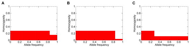
A geometric argument for obtaining the upper and lower bounds on the homozygosity H, as functions of the frequency M of the most frequent allele. In each panel, vertical lines partition the x-axis into a set of allele frequencies with sum equal to 1. Red boxes represent the squares of allele frequencies, and each box indicates the contribution to homozygosity of an individual allele. Homozygosity is represented by the total area in red. The panels depict the case in which M = 0.28 and the number of alleles is K = 7. The dashed line indicates the maximal box height. (A) The maximal H of 0.2608, produced when (p1, p2, p3, p4, p5, p6, p7) = (0.28, 0.28, 0.28, 0.16, 0, 0, 0). (B) An intermediate H of 0.2416, produced when (p1, p2, p3, p4, p5, p6, p7) = (0.28, 0.28, 0.28, 0.04, 0.04, 0.04, 0.04). (C) The minimal H of 0.1648, produced when (p1, p2, p3, p4, p5, p6, p7) = (0.28, 0.12, 0.12, 0.12, 0.12, 0.12, 0.12).
In Theorem 2, given M and K, we seek to partition the x-axis of Figure 1 into at most K components so that the resulting boxes have maximal or minimal area. Comparing Figures 1A and 1B, the two figures differ only in the partition of the interval [0.84, 1]. In Figure 1A, this interval contains a single allele, whereas in Figure 1B, it contains four alleles of equal frequency. The scenario in Figure 1A has greater area, illustrating the principle that because the square of the sum (p1 + p2)2 exceeds the sum of squares , greater area is produced when a larger allele is carved from a fixed interval than when the interval is divided into smaller alleles. This principle that a single box is larger than two boxes that occupy the same total length on the x-axis can be used to show that the maximal area is obtained by proceeding greedily along the x-axis, sequentially separating alleles with frequency M until the remaining length along the axis is less than M, and then choosing a single allele to fill the remaining space. Similarly, the minimum is obtained in the opposite manner, as can be seen in Figure 1C: after choosing one allele with frequency equal to the prespecified maximum M, the minimal sum of squares is produced by subdividing the remaining part of the unit interval into as many small boxes as allowed by the prespecified number of alleles K.
2.2 Proofs of Theorems 1 and 2
To prove the theorems, we use a corollary of the Cauchy-Schwarz inequality.
Lemma 3
Consider a sequence of length K, (a1,…, aK) with ai ≥ 0, such that for some A ≥ 0. Then , with equality if and only if a1 = a2 = … = aK = A/K.
Proof
By the Cauchy-Schwarz inequality, with equality if and only if ai = λ for all i and some constant λ. Because , equality holds if and only if ai = A/K for all i.
In examining the bounds on M in terms of H and on H in terms of M, it is important to take note of the allowable values of H and M. We now show that given the number of alleles K, the homozygosity H and the frequency M of the most frequent allele lie in the interval [1/K, 1).
Lemma 4
At a locus with at most K ≥ 2 alleles, H,M ∈ [1/K, 1).
Proof
By construction, M ∈ (0, 1). Because M ≥ pi for all i, . As pi ∈ [0, 1), . Summing from i = 1 to K, and noting that M2 < M because M ∈ (0, 1), we obtain H < 1. H ≥ 1/K follows from application of Lemma 3 to (p1,…, pK).
We now prove Theorems 1 and 2. We define the upper and lower bound functions on M in terms of H as UMK,LMK : [1/K, 1) → [1/K, 1), respectively, and we define the upper and lower bound functions on H in terms of M as UHK,LHK : [1/K, 1) → [1/K, 1). We aim to determine these functions and to show that they match the formulas in Theorems 1 and 2. For convenience, we denote the corresponding functions in the unspecified-K case, as derived by Rosenberg & Jakobsson (2008) and previously denoted F, f, G, and g, respectively, by UM∞,LM∞,UH∞,LH∞ : (0, 1) → (0, 1).
Proof of Theorem 2
We wish to confirm that for K ≥ 2, UHK(M) = 1 − M(⌈M−1⌉ − 1)(2 − ⌈M−1⌉M) and LHK(M) = (KM2 − 2M + 1)/(K − 1). By Theorem 2ii of Rosenberg & Jakobsson (2008), on the interval [1/K, 1), even if the number of alleles is permitted to exceed K, the upper bound on H is achieved when it is at most K. Thus, UHK(M) = UH∞(M) on [1/K, 1). From eq. A3 of Rosenberg & Jakobsson (2008), UH∞(M) = 1−M(⌈M−1⌉ − 1)(2 − ⌈M−1⌉M), with the appropriate condition for UH∞(M) = H.
By definition, LHK(M) is the minimum of over sequences (p1,…, pK). Because , by Lemma 3, LHK(M) = M2 +(1− M)2/(K − 1), with LHK(M) = H if and only if pi = (1 − M)/(K − 1) for each i with 2 ≤ i ≤ K.
The upper bound UHK(M) for H is equivalent on [1/K, 1) to the corresponding function in the unspecified-K case, UH∞(M). In the unspecified-K case, the upper bound is achieved by choosing ⌈M−1⌉ − 1 alleles to have the highest allele frequency M, and assigning all remaining frequency to one “leftover” allele (see Lemma 3 of Rosenberg & Jakobsson (2008)). Because ⌈M−1⌉ ≤ K on [1/K, 1), in the unspecified-K case, the configuration that achieves the upper bound has K or fewer alleles. The lower bound LHK(M) is attained simply when the remaining frequency after excluding the most frequent allele is distributed equally among the K − 1 remaining alleles. It is easily shown that limK→∞ LHK(M) = LH∞(M) = M2.
Figure 2 superimposes UHK(M) and LHK(M) for K equal to 3, 5, and 15, and in the limiting case of unspecified K. The figure depicts the different domains for different K, and the piecewise structure for UHK. It also illustrates that the bounds are monotonically increasing, continuous, and bijective.
Figure 2.

Upper bounds UHK (solid) and lower bounds LHK (dashed) on the homozygosity H, as functions of the frequency of the most frequent allele. The bounds for loci with K = 3, K = 5, and K = 15 alleles are plotted in red, purple, and blue, respectively, each with domain [1/K, 1). The bounds for the case of unspecified K are plotted in black, with domain (0, 1). The various curves for the upper bound overlap.
Lemma 5
UHK,LHK : [1/K, 1) → [1/K, 1) are monotonically increasing, continuous, and bijective.
Proof
For UHK, the result follows from Lemma 4i of Rosenberg & Jakobsson (2008). The function LHK is a (continuous) quadratic function with positive leading coefficient K/(K − 1). The vertex of LHK occurs at the endpoint M = 1/K; thus, the function LHK is monotonically increasing over [1/K, 1). Because LHK(1/K) = 1/K and LHK(1) = 1, the domain and range of the function are identical.
As a consequence of Lemma 5, UHK and LHK have well-defined inverse functions over [1/K, 1), such that are monotonically increasing, continuous, and bijective. To establish the upper and lower bounds of M in terms of H, we use the invertibility of UHK and LHK over [1/K, 1).
Corollary 6
For K ≥ 2, the inverse functions of UHK and LHK are
| (2) |
| (3) |
Proof
It is easy to check that the function in eq. 3 satisfies . For each k ∈ [2,K], for M in Ik, the function in eq. 2 satisfies .
Proof of Theorem 1
It suffices to confirm that on [1/K, 1), UMK(H) and LMK(H), defined as the upper and lower bounds on M in terms of H, satisfy and .
That follows from Lemma 5 of Rosenberg & Jakobsson (2008). To obtain UMK(H), consider H ∈ [1/K, 1). Rewriting eq. 1 as , M is maximized when is minimized. By Lemma 3, at the minimum, H = M2 +(1−M)2/(K − 1). Solving for M, we take the larger root so that M will be the frequency of the most frequent allele.
The various functions appear in Table 1. Just as Theorem 2 finds that for M ∈ [1/K, 1), UHK(M) = UH∞(M), Theorem 1 finds that for H ∈ [1/K, 1), LMK(H) = LM∞(H). Similarly, just as limK→∞ LHK(M) = LH∞(M) = M2, it is easily shown that .
Table 1.
The functions defining the bounds on homozygosity H and the frequency of the most frequent allele M, given the maximal number of alleles K (left), and in the limiting case of unspecified K (right).
| Function | Definition | Limiting function | Definition | ||
|---|---|---|---|---|---|
| UHK | 1 −M(⌈M−1⌉ − 1)(2 − ⌈M−1⌉M) | UH∞ | Same as UHK | ||
| LHK |
|
LH∞ | M2 | ||
| UMK |
|
UM∞ |
|
||
| LMK |
|
LM∞ | Same as LMK |
Figure 3 plots the upper and lower bounds on M in terms of H, with K equal to 3, 5, and 15, and in the limiting unspecified-K case. Comparing Figures 2 and 3, it is visually apparent that the lower bound of M and the upper bound of H are inverse functions, as are the upper bound of M and the lower bound of H.
Figure 3.

Upper bounds UMK (dashed) and lower bounds LMK (solid) on the frequency M of the most frequent allele, as functions of homozygosity. The bounds for loci with K = 3, K = 5, and K = 15 alleles are plotted in red, purple, and blue, respectively, each with domain [1/K, 1). The bounds for the case of unspecified K are plotted in black, with domain (0, 1). The various curves for the lower bound overlap. The upper and lower bounds in this figure are inverse functions of the lower and upper bounds in Figure 2.
3 Features of the bounds on M in terms of H
We next highlight some of the features of the upper and lower bounds identified in Theorems 1 and 2. For many of our results, when applying a limit as K → ∞, we obtain corresponding results from the unspecified-K case of Rosenberg & Jakobsson (2008). Although the input value H = 1 or M = 1 does not represent a polymorphic genetic locus, it is convenient to view UMK and LMK as producing output M = 1 at H = 1 and UHK and LHK as producing H = 1 at M = 1. First, we consider the upper and lower bounds on the frequency of the most frequent allele M in terms of homozygosity H, as obtained in Theorem 1.
3.1 Mean values of the bounds
Proposition 7
For K ≥ 2, averaging across values of H ∈ [1/K, 1), (i) the mean of UMK(H) is 2/3+1/(3K); (ii) the mean of LMK(H) is ; (iii) the mean of UMK(H) − LMK(H) is .
Proof
-
and simplify to −1 + 1/K and , respectively.
This result follows by taking the difference between the results in parts i and ii.
Proposition 8
For K ≥ 2, averaging across values of H ∈ [1/K, 1), (i) the mean of UMK(H) − H is 1/6 − 1/(6K); (ii) the mean of LMK(H) − H is .
Proof
By Lemma 7 of Rosenberg & Jakobsson (2008), on the interval [1/K, 1), LMK(H) ≥ H. Averaging over H ∈ [1/K, 1), the mean of H is 1/2+1/(2K). We subtract this expression from the results in parts i and ii of Proposition 7 to acquire the means of UMK(H) − H and LMK(H) − H, respectively.
By noting that , we can observe that as K → ∞, the limiting values in the three parts of Proposition 7 approach the corresponding values in Proposition 6 of Rosenberg & Jakobsson (2008): 2/3, π2/18, and 2/3 − π2/18, respectively. Similarly, the limits in Proposition 8 approach the quantities in Proposition 8 of Rosenberg & Jakobsson (2008): 1/6 and π2/18 − 1/2.
It is also noteworthy that the mean difference UMK(H) − LMK(H) for a fixed K is always smaller than the large-K limiting mean difference. Thus, when incorporating the value of K, the interval in which M is confined by its upper and lower bounds has a narrower range than in the case of K unspecified. We can measure the mean improvement that specification of K provides in ascertaining M given H, by evaluating the difference between the mean difference of the upper and lower bounds of M with K unspecified and the reduced mean difference of the upper and lower bounds for fixed finite K.
Proposition 9
For K ≥ 2, averaging across values of H ∈ [1/K, 1), (i) the mean of UM∞(H) − LM∞(H) is ; (ii) the mean difference between UM∞(H) − LM∞(H) and UMK(H) − LMK(H) is .
Proof
-
iUsing Proposition 7ii to obtain the mean of LMK(H), which equals LM∞(H) on [1/K, 1), the result follows by simplifying
-
ii
The result follows by subtracting the result in Proposition 7iii from the result in i.
As K → ∞, the limiting values in Proposition 9i and ii approach 2/3 − π2/18 and 0, respectively. These results are sensible: as K → ∞, the set of allowed values of H approaches (0, 1), so that the mean of UM∞(H)−LM∞(H) over [1/K, 1) approaches its mean over the entire interval (0, 1). UMK(H) − LMK(H) approaches UM∞(H) − LM∞(H), so the mean of UMK(H) − LMK(H) approaches the mean of UM∞(H) − LM∞(H).
For K equal to 3, 5, and 15, Figure 4 plots the areas that are lost from the unspecified-K case in refining the upper bound on M given specified values of K. For K equal to 2, 3, 4, 5, and 15, evaluating the quantity in Proposition 9ii, the reductions in the mean difference between the upper and lower bounds on M are approximately 0.0286, 0.0298, 0.0278, 0.0255, and 0.0131, respectively. These values are not insignificant fractions of 0.1184, the mean difference between the upper and lower bounds on M over the whole unit interval in the case of K unspecified. The maximal improvement occurs at K = 3, accounting for ~25% of the total area between UM∞(H) and LM∞(H).
Figure 4.

The refinement in the range for the frequency of the most frequent allele as a function of homozygosity, when K is specified compared to unspecified. The red, purple, and blue regions correspond to the reductions in range for K = 3, K = 5, and K = 15, respectively.
3.2 Maximal and minimal differences between the bounds
Figure 5 plots the pairwise differences between the upper bound of M, the lower bound of M, and H itself. We now prove a variety of results about UMK(H), LMK(H), and H, based on patterns visible in the figure.
Figure 5.

The difference between the upper and lower bounds on the frequency of the most frequent allele, for a given homozygosity, and the difference between the bounds and homozygosity itself. (A) UMK(H) − H. (B) LMK(H) − H. (C) UMK(H) − LMK(H). (D) Superposition of parts (A), (B), and (C). Plots for loci with K = 3, K = 5, and K = 15 alleles appear in red, purple, and blue, respectively, each with domain [1/K, 1). The case of unspecified K is plotted in black, with domain (0, 1).
In Figure 5A, we notice that the difference between the upper bound of M and H has a single maximal value within [1/K, 1). The following proposition identifies the location of this point.
Proposition 10
On [1/K, 1), the maximal value of UMK(H) − H is (K − 1)/(4K), and it is achieved at H = (K + 3)/(4K).
Proof
The derivative of UMK(H)−H with respect to H, , has a single critical point at ((K + 3)/(4K), (K − 1)/(4K)). The second derivative of UMK(H) − H is negative over the entire domain, so that UMK(H) − H achieves a global maximum at the critical point.
As K → ∞, the maximum of UMK(H) − H approaches (1/4, 1/4), the location of the maximum of UM∞(H) − H, as derived in Corollary 13 of Rosenberg & Jakobsson (2008) for the case of unspecified K.
Figure 5B plots the difference LMK(H) − H. As shown in Proposition 9 of Rosenberg & Jakobsson (2008), because LMK(H) = LM∞(H) on Ik for k ≤ K, the local maximum of LMK(H)−H in Ik occurs at ((4k−3)/[4k(k− 1)], 1/[4k(k−1)]). As shown in Corollary 10 of Rosenberg & Jakobsson (2008), considering all k with 2 ≤ k ≤ K, the highest of the local maxima is achieved at (5/8, 1/8).
In Figure 5C, we observe that the difference between the upper and lower bounds of M has a series of local minima, with maxima occurring at reciprocals of integers. We now derive the locations of the minima.
Proposition 11
Suppose K ≥ 3. On [1/k, 1/(k − 1)], for k ∈ [2,K], the minimal value of UMK(H) − LMK(H) occurs at H = [(k − 1)(K − 1) − 1]/[k(k − 1)(K − 1) − K], and is
Proof
If k = K = 2, then UMK(H) = LMK(H). Otherwise, . The only critical value occurs at H = [(k −1)(K − 1)− 1]/[k(k− 1)(K − 1)− K], which we denote by φ(K, k). This value lies in the interior of [1/k, 1/(k − 1)], except if k = K, for which it lies at the left endpoint, and for k = 2, for which it lies at the right endpoint.
To verify that this critical value is a minimum, we evaluate the second derivative of UMK(H) − LMK(H):
The second derivative is positive at H if . At H = φ(K, k), (KH − 1)/(kH − 1) = (K − 1)(k − 1), from which it follows that the second derivative is positive at H = φ(K, k) if K/(K − 1) < k(k − 1). For K ≥ k ≥ 2 and K ≥ 3, K/(K − 1) < 2 and k(k − 1) ≥ 2. Thus, H = φ(K, k) is a minimum.
Taking the limit of φ(K, k) as K → ∞ yields (k − 1)/(k2 − k − 1), the location of the minimum of UM∞(H) − LM∞(H) on H ∈ [1/k, 1/(k − 1)] according to Proposition 11ii of Rosenberg & Jakobsson (2008). The value of UMK(H)−LMK(H) at the minimum approaches , the minimum of UM∞(H) − LM∞(H) on [1/k, 1/(k − 1)].
We now identify the location of the highest of the local minima of UMK(H)− LMK(H).
Proposition 12
Suppose K ≥ 4. On [1/K, 1], the highest local minimum of UMK(H) − LMK(H) occurs at H = φ(K, 3) for K ∈ {4, 5}, at both H = φ(K, 3) and H = φ(K, 4) for K = 6, at H = φ(K, 4) for K ∈ [7, 17], and at H = φ(K, 5) for K ≥ 18.
Proof
By Proposition 11, we aim to find the maximal value among local minima that occur at (φ(K, k),UMK(φ(K, k))−LMK(φ(K, k))), for integers k ∈ [3,K −1]. The interval [1/k, 1/(k −1)] has no interior local minimum for k = 2 or k = K. Thus, for K = 2 and K = 3 there are no nonzero minima, and for K = 4 the only nonzero minimum occurs at φ(4, 3).
Consider K ≥ 5. For k ≠ 2 and k ≠ K, the proof of Proposition 11 shows that each interval [1/k, 1/(k − 1)] has a single interior critical point for UMK(H) − LMK(H), and that this point is a minimum. As a result, the maximum of the function must occur at one of the endpoints of the interval. Thus, given K, if there exist values of k and J such that UMK(φ(K, k))− LMK(φ(K, k)) exceeds UMK(1/j)−LMK(1/j) for all j ≥ J, then UMK(φ(K, k))−LMK(φ(K, k)) exceeds the local maxima — and consequently, the local minima — on all intervals [1/j, 1/(j − 1)] for all j > J. It can be shown that UMK(φ(K, 5))−LMK(φ(K, 5)) exceeds UMK(1/7)−LMK(1/7) for all K ≥ 7.
Denoting αK(m, n) = [UMK(φ(K,m))−LMK(φ(K,m))]−[UMK(φ(K, n))−LMK(φ(K, n))], it can be shown that αK(5, 6) > 0 for all K ≥ 6, and αK(5, 7) > 0 for all K ≥ 7. Thus, for all K ≥ 4, the desired maximum among the local minima occurs at φ(K, k) for some k ≤ 5.
It can be shown that αK(3, 4) > 0 for K = 5, αK(3, 4) = 0 for K = 6, αK(4, 5) > 0 for K ∈ [5, 17], αK(4, 3) > 0 for K ≥ 7, and αK(5, 4) > 0 for K ≥ 18.
For large K, the highest local minimum of UMK(H) − LMK(H) occurs at φ(K, 5) = 4/19, the location of the highest local minimum of UM∞(H) − LM∞(H) by Proposition 12 of Rosenberg & Jakobsson (2008).
We next consider the maxima of the difference UMK(H)−LMK(H). First we find the global maximum. We then examine the locations of the local maxima in intervals [1/k, 1/(k − 1)].
Proposition 13
Suppose K ≥ 3. On [1/K, 1], the maximal value of UMK(H)− LMK(H) occurs at H = 1/2 for K ∈ {3, 4}, at H = 1/3 for K ∈ [5, 18], and at H = 1/4 for K ≥ 19.
Proof
For K = 2, UMK(H) − LMK(H) = 0. For K ≥ 3, local maxima of UMK(H) − LMK(H) occur at integers 1/k, where UMK(H) − LMK(H) coincides with UMK(H) − H. By Proposition 10, the global maximum of UMK(H) − H, which has a single critical value, occurs at (K + 3)/(4K). Consequently, the highest local maximum of UMK(H) − LMK(H) occurs at one of the endpoints of the interval for which 1/k ≤ (K+3)/(4K) ≤ 1/(k−1), that is, the interval on whose interior k = ⌈4K/(K + 3)⌉.
If K = 3, (K +3)/(4K) is exactly equal to 1/2, and UMK(H)−LMK(H) is therefore maximized at 1/2. Similarly, if K = 9, (K + 3)/(4K) = 1/3, and UMK(H) − LMK(H) is maximized at 1/3. For all other K, the global maximum of UMK(H) −H at (K + 3)/(4K) occurs interior to some interval [1/k, 1/(k − 1)]: [1/2, 1/3] for K ∈ [4, 8] and [1/3, 1/4] for K ≥ 10.
For K ≠ 3 and K ≠ 9, to determine whether UMK(1/k) − LMK(1/k) is maximized at k = 2 or k = 3, we define ψ(K, k) = [UMK(1/k) − 1/k] − [UMK(1/(k−1))−1/(k−1)]. ψ(4, 3) < 0, but ψ(K, 3) > 0 for K ∈ {5, 6, 7, 8}. Therefore, the global maximum of UMK(H) − LMK(H) for K = 4 occurs at H = 1/2, and for K ∈ [5, 8], it occurs at H = 1/3.
For K ≥ 10, it can be shown that the function ψ(K, 4) is negative until its single root at K ≈ 18.83, and positive thereafter. Consequently, the global maximum of UMK(H) − LMK(H) for K ∈ [10, 18] occurs at H = 1/3, and for K ≥ 19, it occurs at H = 1/4.
For large K, the location of the maximal difference between the upper and lower bounds of M is at H = 1/4, as in the unspecified-K case in Corollary 14 of Rosenberg & Jakobsson (2008).
Proposition 14
Suppose K ≥ 3. On [1/k, 1/(k − 1)], for k ∈ [2,K], the maximal value of UMK(H)−LMK(H) occurs (i) at H = 1/k if k < ⌈4K/(K+ 3)⌉, (ii) at H = 1/(k − 1) if k > ⌈4K/(K + 3)⌉, and (iii) at the location in Table 2 if k = ⌈4K/(K + 3)⌉.
Table 2.
The location of the maximum of UHK(M)−LHK(M) on [1/k, 1/(k−1)], when k = ⌈4K/(K + 3)⌉. The table is part of the statement of Proposition 14.
| K | k = ⌈4K/(K + 3)⌉ | Location of maximum of UHK(M) − LHK(M) on [1/k, 1/(k −1)]
|
|
|---|---|---|---|
| Interval endpoint | Value | ||
| 3 | 2 | 1/k | 1/2 |
| 4 | 3 | 1/(k − 1) | 1/2 |
| 5, 6, 7, 8, 9 | 3 | 1/k | 1/3 |
| 10, 11,…, 18 | 4 | 1/(k − 1) | 1/3 |
| ≥ 19 | 4 | 1/k | 1/4 |
Proof
By Lemma 7 of Rosenberg & Jakobsson (2008), UMK(H)−LMK(H) ≤ UMK(H) − H, with equality if and only if H = 1/k for integers k ∈ [2,K]. By Proposition 10, UMK(H)−H is increasing over [1/K, (K +3)/(4K)] and decreasing over [(K + 3)/(4K), 1]. Proposition 11 shows that UMK(H) − LMK(H) has at most one critical value on [1/k, 1/(k − 1)], a local minimum. Thus, the maximal value of UMK(H) − LMK(H) on the interval occurs at one of the endpoints, where UMK(H) − LMK(H) has the same values as UMK(H) − H. For k < ⌈4K/(K + 3)⌉, the maximum occurs at 1/k, and for k > ⌈4K/(K + 3)⌉, it occurs at 1/(k − 1). If k = ⌈4K/(K + 3)⌉, then the maximum occurs at the global maximum of UMK(H) − LMK(H) over [1/K, 1], whose location, derived in Proposition 13, is given in Table 2.
As K → ∞, the maximum on [1/k, 1/(k−1)] occurs at 1/(k−1) for k > 4 and at 1/k for k ≤ 4. This limit agrees with the result in Proposition 11i of Rosenberg & Jakobsson (2008) for UM∞(H) − LM∞(H).
In Figure 5D, we notice that the difference between the upper and lower bounds of M intersects the difference between the lower bound of M and H at a coordinate within the interval [1/2, 1). In the following proposition, we analyze the behavior of UMK(H) − LMK(H) and LMK(H) − H.
Proposition 15
Suppose K ≥ 3. Define R(K) to be the location of the single root of that lies in (1/2, 1). Then the difference UMK(H)−LMK(H) is (i) greater than LMK(H)−H if 1/K < H < R(K); (ii) equal to LMK(H) − H if H ∈ {1/K,R(K), 1}; (iii) less than LMK(H) − H if R(K) < H < 1.
Proof
We show that UMK(H) − LMK(H) ≥ LMK(H) − H for H ∈ Ik and k ∈ [3,K], with equality if and only if H = 1/K. In interval IK,
| (4) |
Eq. 4 is 0 for H = 1/K. Elsewhere on IK, is positive, and for K ≥ 3.
For H ∈ [1/K, 1), if K′ > K, then UMK′ (H) > UMK(H) and LMK′ (H) = LMK(H). Consider an interval Ik, for k ∈ [3,K′]. For k = K′, UMK′ (H) − LMK′ (H) ≥ LMK′ (H) − H on Ik, with equality if and only if H = 1/K′, based on the argument in the previous paragraph with K′ in place of K. For k ∈ [3,K′ − 1], (UMK′ (H) − LMK′ (H)) − (LMK′ (H) − H) > (UMk(H) − LMk(H)) − (LMk(H) − H) on the interval Ik. But (UMk(H) − LMk(H)) − (LMk(H)−H) > 0 based on the argument in the previous paragraph with k in place of K. Thus, we can conclude that for all K ≥ 3, UMK(H)−LMK(H) ≥ LMK(H) − H for H ∈ [1/K, 1/2), with equality if and only if H = 1/K.
Now consider k = 2, for which H ∈ [1/2, 1]. On this interval,
| (5) |
For each K ≥ 3, this function is positive at H = 1/2, negative at H = 1−1/K, and zero at H = 1. It is straightforward to show that its second derivative is positive on [1/2, 1]. We can therefore conclude that eq. 5 has a single zero interior to (1/2, 1). The location of this zero does not have a convenient formula, and we simply label it R(K). Because (UMK(H) − LMK(H)) − (LMK(H) − H) is continuous and is positive at H = 1/2, it switches from positive to negative at H = R(K) before reaching zero again at H = 1.
As K → ∞, R(K) becomes the single root of that lies in (1/2, 1), or . The result then accords with the unspecified-K case in Proposition 15 of Rosenberg & Jakobsson (2008).
4 Features of the bounds on H in terms of M
We now turn our attention to the various properties of the upper and lower bounds of H, UHK and LHK, in terms of M. As in the case of the bounds on M in terms of H in Section 3, we begin by examining the means of the upper and lower bounds over the interval [1/K, 1).
4.1 Mean values of the bounds
Proposition 16
For K ≥ 2, averaging across values of M ∈ [1/K, 1), (i) the mean of UHK(M) is ; (ii) the mean of LHK(M) is 1/3 + 2/(3K); (iii) the mean of UHK(M) − LHK(M) is .
Proof
-
iii
Using the inverse relationships between UHK(M) and LMK(H) and between LHK(M) and UMK(H), the area between UHK(M) and LHK(M) is identical to the area between UMK(H) and LMK(H). The result follows from Proposition 7iii.
-
ii
.
-
i
The result follows by summing the results in parts ii and iii.
Proposition 17
For K ≥ 2, averaging across values of M ∈ [1/K, 1), (i) the mean of M − UHK(M) is ; (ii) the mean of M − LHK(M) is 1/6 − 1/(6K).
Proof
By Lemma 18 of Rosenberg & Jakobsson (2008), M ≥ UHK(M). Subtracting the result of Proposition 16i from , the result follows.
The result follows by summing the results in part i and Proposition 16iii.
Taking the limits as K → ∞ for the results in Proposition 16, we obtain 1−π2/18, 1/3, and 2/3−π2/18, respectively, as in Proposition 17 of Rosenberg & Jakobsson (2008). Similarly, the limits of π2/18−1/2 and 1/6 in Proposition 17i and ii agree with Proposition 19 of Rosenberg & Jakobsson (2008).
As in the case of the bounds on M, we can compute the reduction in mean difference between the upper and lower bounds on H yielded by specifying K.
Proposition 18
For K ≥ 2, averaging across values of M ∈ [1/K, 1), (i) the mean of UH∞(M)−LH∞(M) is ; (ii) the mean difference between UH∞(M) − LH∞(M) and UHK(M) − LHK(M) is (K − 1)/(3K2).
Proof
-
ii
Noting that UH∞(M) = UHK(M), the desired mean reduces to . Subtracting from the quantity in Proposition 16ii, the result follows.
-
i
This result follows by summing the results in part ii and Proposition 16iii.
As K → ∞, the limiting values in Proposition 18i and ii approach 2/3 − π2/18 and 0, respectively. These results are sensible, as the region represented in Proposition 18i approaches the region between UH∞ and LH∞ over the whole unit interval, a region with area 2/3−π2/18. The region in Proposition 18ii becomes progressively smaller as the region between UHK and LHK approaches the region between UH∞ and LH∞.
For K equal to 3, 5, and 15, Figure 6 plots the areas lost in refining the upper bound of H given K compared to the case of K unspecified. For K equal to 2, 3, 4, 5, and 15, using Proposition 18ii, the reductions in the mean difference between the upper and lower bounds on M are approximately 0.0833, 0.0741, 0.0625, 0.0533, and 0.0207, respectively. Especially for small K, these values provide substantial reductions compared to 0.1184, the mean difference between the upper and lower bounds on H over (0, 1) when K is unspecified. The largest reduction occurs for K = 2.
Figure 6.

The refinement in the range for homozygosity as a function of the frequency of the most frequent allele, when K is specified compared to unspecified. The red, purple, and blue regions correspond to the reductions in range for K = 3, K = 5, and K = 15, respectively.
4.2 Maximal and minimal differences between the bounds
Figure 7 plots the differences among the upper bound of H, the lower bound of H, and M itself. We now examine the properties of the local maxima and minima visible in the figure.
Figure 7.

The difference between the upper and lower bounds on homozygosity, for a given frequency of the most frequent allele, and the difference between the frequency of the most frequent allele and the bounds. (A) M − UHK(M). (B) M − LHK(M). (C) UHK(M) − LHK(M). (D) Superposition of parts (A), (B), and (C). Plots for loci with K = 3, K = 5, and K = 15 alleles appear in red, purple, and blue, respectively, each with domain [1/K, 1). The case of unspecified K is plotted in black, with domain (0, 1).
The difference between M and the upper bound of H is the same for specified K as for K unspecified, except with a different domain. Thus, in Figure 7A, which plots the difference between M and the upper bound of H, a local maximum occurs in each interval [1/k, 1/(k − 1)] for 2 ≤ k ≤ K, as in Proposition 20 of Rosenberg & Jakobsson (2008). This maximum occurs at ((2k − 1)/[2k(k − 1)], 1/[4k(k − 1)]). As in Corollary 21 of Rosenberg & Jakobsson (2008), the highest maximum occurs at (3/4, 1/8), when k = 2.
In Figure 7B, which plots the difference between M and the lower bound of H, we notice that a single maximum value occurs in the domain [1/K, 1). We now establish the location of this maximum.
Proposition 19
On [1/K, 1), the maximal value of M − LHK(M) is 1/4 − 1/(4K), and it is achieved at M = 1/2 + 1/(2K).
Proof
M − LHK(M) = [−KM2 + (K + 1)M − 1]/(K − 1). The vertex of this parabola is at M = (K + 1)/(2K), which necessarily lies in the interior of [1/K, 1).
The location of the maximum is at the midpoint of the interval [1/K, 1), and M − LHK(M) is zero at the endpoints 1/K and 1. As K → ∞, the location of the maximum approaches (1/2, 1/4), the location of the maximum of M − LH∞(M) in Corollary 24 of Rosenberg & Jakobsson (2008).
Figure 7C plots the difference between the upper and lower bounds of H. For K ≥ 3 and 3 ≤ k ≤ K − 1, this curve has an interior local minimum in the interval [1/k, 1/(k − 1)].
Proposition 20
Suppose K ≥ 3. On [1/k, 1/(k − 1)], for k ∈ [2,K], the minimal value of UHK(M)−LHK(M) occurs at M = [k(K −1) − K]/[k(k − 1)(K − 1) − K], and is [(k − 2)(K − k)]/[k(k − 1)(K − 1) − K].
Proof
On [1/k, 1/(k − 1)], . Excluding the case of k = K = 2, this function is a parabola with positive leading coefficient, whose vertex is at M = [k(K − 1) − K]/[k(k − 1)(K − 1) − K]. Except if k = 2 or k = K, this point lies in the interior of the interval [1/k, 1/(k −1)]; if k = K, it lies at the left endpoint, and if k = 2, it lies at the right endpoint. At the minimum, the value of UHK(M)−LHK(M) is (k −2)(K−k)/[k(k −1)(K −1)−K]. This minimum is zero in the leftmost interval, with k = K, and in the rightmost interval, with k = 2.
As K → ∞, the locations of the local minima approach ((k −1)/(k2−k− 1), (k − 2)/(k2 − k − 1)). These locations match those found for UH∞(M) − LH∞(M) in Proposition 22ii of Rosenberg & Jakobsson (2008).
We now identify the location of the greatest local minimum of UHK(M)− LHK(M).
Proposition 21
Suppose K ≥ 4. On [1/K, 1], the highest local minimum of UHK(M) − LHK(M) is (K − 3)/(5K − 6), and it occurs at M = (2K − 3)/(5K − 6).
Proof
For 2 ≤ k ≤ K, each interval [1/k, 1/(k − 1)] has an interior local minimum, except if k = 2 or k = K. Thus, no interior local minima occur for K = 2 or K = 3, and we only consider K ≥ 4. Using Proposition 20, define ωK(k) as the minimum value of UHK(M)−LHK(M) over the interval [1/k, 1/(k − 1)]. We show that among integers k with 3 ≤ k ≤ K − 1, ωK(k) is maximal at k = 3:
For K ≥ 4 and k ≥ 3, the denominator is positive. For k ≥ 3 and K ≥ k, the numerator is positive. Thus, as ωK(k) > ωK(k + 1), k = 3 produces the maximal value of ωK(k), at the location in Proposition 20.
As K → ∞, the limiting location of the highest of the local minima is at (2/5, 1/5), the location of the highest local minimum of UH∞(M)−LH∞(M) in Proposition 23 of Rosenberg & Jakobsson (2008).
Our next result examines local maxima of UHK(M) − LHK(M).
Proposition 22
Suppose K ≥ 3. On [1/k, 1/(k−1)], for k ∈ [3,K], the maximal value of UHK(M) − LHK(M) is (k − 2)(K − k + 1)/[(k − 1)2(K − 1)], and it is achieved at M = 1/(k−1); if k = 2, the maximal value of UHK(M)− LHK(M) is (K − 2)/[4(K − 1)], and it is achieved at M = 1/2.
Proof
The maximum must occur at one of the two endpoints of the interval. For integers k with 2 ≤ k ≤ K, UHK(1/k) = 1/k. At M = 1/k, UHK(M) − LHK(M) = (k − 1)(K − k)/[k2(K − 1)], and at M = 1/(k − 1), UHK(M) − LHK(M) = (k − 2)(K − k + 1)/[(k − 1)2(K − 1)]. It is straightforward to show that the latter value is greater than the former for k ≥ 3 and K ≥ k, and that the reverse is true for k = 2.
Corollary 23
Suppose K ≥ 3. On [1/K, 1], the maximal value of UHK(M)− LHK(M) is (K − 2)/[4(K − 1)], and it is achieved at M = 1/2.
Proof
By Proposition 22, the local maxima of UHK(M)−LHK(M) occur at points 1/k for 2 ≤ k < K. At such points, UHK(M) = M. From Proposition 19, M − LHK(M) is increasing on [1/K, 1/2 + 1/(2K)]. Thus, considering points 1/k where k is an integer with 2 ≤ k < K, the maximum of UHK(M)− LHK(M) occurs at M = 1/2.
As K → ∞, local maxima occur at (1/(k −1), (k −2)/(k − 1)2) for k > 2, and at (1/2, 1/4) for k = 2. These locations accord with Proposition 22i of Rosenberg & Jakobsson (2008). The global maximum approaches (1/2, 1/4), the location in Corollary 25 of Rosenberg & Jakobsson (2008).
In Figure 7D, we notice that the curves in Figures 7B and 7C coincide at reciprocals of integers, while the curves in Figures 7A and 7C coincide only in the two intervals (1/K, 1/(K −1)) and (1/2, 1) for K ≥ 3. We now determine the precise locations where M−UHK(M) and UHK(M)−LHK(M) intersect.
Proposition 24
Suppose K ≥ 3. Define S(K) = (2K − 3)/(2K2 − 4K + 1) and T(K) = (2K−3)/(3K−4). Then the difference UHK(M)−LHK(M) is (i) greater than M−UHK(M) if S(K) < M < T(K); (ii) equal to M−UHK(M) if M ∈ {1/K, S(K), T(K), 1}; (iii) less than M − UHK(M) if 1/K < M < S(K) or T(K) < M < 1. The intersection points of UHK(M) − LHK(M) and M−UHK(M) interior to [1/K, 1] occur at (S(K), (K−1)(K−2)/(2K2− 4K + 1)2) and (T(K), (K − 1)(K − 2)/(3K − 4)2).
Proof
In each interval [1/k, 1/(k − 1)] for k > 2, by Proposition 20, the minimal value of UHK(M)−LHK(M) is (k−2)(K−k)/[k(k−1)(K−1)−K]. By Proposition 20 of Rosenberg & Jakobsson (2008), the maximal value of M − UHK(M) is 1/[4k(k − 1)].
We show that except if k = K or k = 2, the minimum of UHK(M) − LHK(M) exceeds the maximum of M − UHK(M). Writing ζ(K, k) = (k − 2)(K − k)/[k(k − 1)(K − 1) − K] − 1/[4k(k − 1)], substituting c = K − k where 1 ≤ c ≤ K − 3, and simplifying, it follows that ζ(K, k) > 0 if η(c, k) = (4c − 1)k3 + (2 − 13c)k2 + 9ck + c > 0. For k = 3, η(c, k) = 19c − 9, which exceeds 0 because c ≥ 1.
The difference η(c, k +1)−η(c, k) is equal to (12c−3)k2 +(1−14c)k +1. Because c ≥ 1, 12c − 3 ≥ 9c. Consequently, η(c, k + 1) − η(c, k) ≥ (9k − 14)ck + k + 1, which exceeds 0 for k ≥ 3. Thus, because η(c, 3) > 0 and η(c, k + 1) > η(c, k) for k ≥ 3, it follows that UHK(M) − LHK(M) exceeds M − UHK(M) over [1/k, 1/(k − 1)] for 3 ≤ k ≤ K − 1.
Setting k = K, UHK(M)−LHK(M) < M −UHK(M) if K(2K2 −4K + 1)M2 − (4K2 − 7K + 1)M + (2K − 3) < 0, that is, if M lies in (1/K, S(K)). The intersection points for UHK(M) − LHK(M) and M − UHK(M) on [1/K, 1/(K−1)] occur at (1/K, 0) and (S(K), (K−1)(K−2)/(2K2−4K+1)2).
Setting k = 2, UHK(M)−LHK(M) < M−UHK(M) if (3K−4)M2+(7− 5K)M +(2K −3) < 0, that is, if M lies in (T(K), 1). The intersection points for UHK(M)−LHK(M) and M−UHK(M) on [1/2, 1] occur at (T(K), (K− 1)(K − 2)/(3K − 4)2) and (1, 0).
As K → ∞, the intersection points at S(K) and T(K) approach (0, 0) and (2/3, 1/9), respectively. Thus, the limiting result agrees with Proposition 26 of Rosenberg & Jakobsson (2008).
5 Application to Data
Our mathematical results are informative for examining homozygosity and the frequency of the most frequent allele in multiallelic population-genetic data. We considered the values of H, M, and K for 783 microsatellite loci in 1048 individuals from worldwide human populations (Rosenberg et al., 2005), treating allele frequency estimates as parametric allele frequencies. To illustrate the effect of K on the bounds on H in terms of M and M in terms of H, we show results for two distinct values of K, K = 7 and K = 15.
Superimposing the graphs of UM15(H) and UM7(H) along with graphs of UM∞(H) and LM∞(H), we can see in Figure 8 that for the 27 loci with K = 7 alleles, M and H tend to be greater than for the 33 loci with K = 15 alleles. In some cases, loci with K = 15 alleles have values of M and H that do not lie in the allowed region for loci with K = 7 alleles. Both for K = 7 and for K = 15, the region between UMK(H) and LMK(H) circumscribes the points plotted for loci with the given value of K more precisely than does the region between UM∞(H) and LM∞(H).
Figure 8.

Frequency of the most frequent allele and homozygosity for 27 loci with K = 7 alleles (purple circles) and 33 loci with K = 15 alleles (blue crosses). The plot shows the upper and lower bounds on M given H for K = 7 (purple) and K = 15 (blue) alleles, and in the case of unspecified K (black).
6 Discussion
By considering the value of the number of alleles at a locus in evaluating the relationship between homozygosity and the frequency of the most frequent allele, we have refined the range in which one of the two quantities must lie when the other is given. Our analysis extends the work of Rosenberg & Jakobsson (2008) on the case of unspecified K, and indeed, it can be used to obtain many of the earlier results by taking limits as K → ∞.
Rosenberg & Jakobsson (2008) identified several examples in which the relationship between H and M could be used to understand the behavior of haplotype frequency statistics relying on H or M in tests of neutrality using haplotype frequencies in a population. Our refinements in range for H given M and M given H when K is specified provide an improved basis for interpreting population-genetic statistics based on H and M. These refinements can be particularly helpful in comparing inferences based on loci with different numbers of alleles, for which the precise relationship between H and M will differ. Additionally, they can also be useful in cases in which H, M, and K are measured from sample frequency distributions, as in our human microsatellite example. In this context, treating sample frequencies as parametric frequencies, the number of observations at a locus is an upper bound on K. As the range reduction for H given M or M given H owing to specification of K is maximal when K is small (Propositions 9 and 18), when H, M, and K are obtained from small samples, the bounds in this article can potentially provide a noticeable improvement compared to earlier work.
Our results trace largely to the fact that the allele frequencies at a locus constitute a set of nonnegative numbers with sum equal to 1. This property of allele frequencies has a variety of mathematical consequences not only for homozygosity and heterozygosity, but also for measures of differentiation across populations (Long & Kittles, 2003; Hedrick, 2005; Jost, 2008) and measures of association among loci (Rosenberg & Calabrese, 2004; Wray, 2005; VanLiere & Rosenberg, 2008). In each of these various situations, mathematical understanding of the underlying properties of population-genetic statistics provides insights into the ways in which the statistics behave when applied in data analysis. Thus, our work on homozygosity and the frequency of the most frequent allele, beyond providing new results on their specific relationship, can be seen in a broader context as a new addition to the mathematical theory of the fundamental statistics of population genetics.
Acknowledgments
The authors gratefully acknowledge two reviewers for detailed comments, T. Pemberton for technical assistance, and the Burroughs Wellcome Fund and NIH grant GM081441 for financial support.
Contributor Information
Shashir B. Reddy, Center for Computational Medicine and Bioinformatics, University of Michigan, 100 Washtenaw Ave, Ann Arbor, MI 48109, USA
Noah A. Rosenberg, Email: rnoah@umich.edu, Department of Human Genetics, Center for Computational Medicine and Bioinformatics, and the Life Sciences Institute, University of Michigan, 100 Washtenaw Ave, Ann Arbor, MI 48109, USA
References
- Hedrick PW. A standardized genetic differentiation measure. Evolution. 2005;59:1633–1638. [PubMed] [Google Scholar]
- Jost L. GST and its relatives do not measure differentiation. Mol Ecol. 2008;17:4015–4026. doi: 10.1111/j.1365-294x.2008.03887.x. [DOI] [PubMed] [Google Scholar]
- Long JC, Kittles RA. Human genetic diversity and the nonexistence of biological races. Hum Biol. 2003;75:449–471. doi: 10.1353/hub.2003.0058. [DOI] [PubMed] [Google Scholar]
- Rosenberg NA, Calabrese PP. Polyploid and multilocus extensions of the Wahlund inequality. Theor Pop Biol. 2004;66:381–391. doi: 10.1016/j.tpb.2004.07.001. [DOI] [PubMed] [Google Scholar]
- Rosenberg NA, Jakobsson M. The relationship between homozygosity and the frequency of the most frequent allele. Genetics. 2008;179:2027–2036. doi: 10.1534/genetics.107.084772. [DOI] [PMC free article] [PubMed] [Google Scholar]
- Rosenberg NA, Mahajan S, Ramachandran S, Zhao C, Pritchard JK, Feldman MW. Clines, clusters, and the effect of study design on the inference of human population structure. PLoS Genet. 2005;1:660–671. doi: 10.1371/journal.pgen.0010070. [DOI] [PMC free article] [PubMed] [Google Scholar]
- VanLiere JM, Rosenberg NA. Mathematical properties of the r2 measure of linkage disequilibrium. Theor Pop Biol. 2008;74:130–137. doi: 10.1016/j.tpb.2008.05.006. [DOI] [PMC free article] [PubMed] [Google Scholar]
- Weir BS. Genetic Data Analysis II. Sinauer; Sunderland, MA: 1996. [Google Scholar]
- Wray NR. Allele frequencies and the r2 measure of linkage disequilibrium: impact on design and interpretation of association studies. Twin Res Hum Genet. 2005;8:87–94. doi: 10.1375/1832427053738827. [DOI] [PubMed] [Google Scholar]