Autonomous Mathematical Reconstruction of Polyethylene Tibial Inserts to Measure Low Wear Volumes

Abstract

Wear of the polyethylene tibial component is a major factor in the success of total knee replacements. However, sampling resolution and the challenges of estimating original surfaces with relatively complex articulating geometries have limited the accuracy of volumetric measurements of wear on surgically retrieved inserts. A mathematical model analyzed volume error due to sampling resolution and found that 100x100μm point spacing reduced error below 1 mm³. Small volumes of material were progressively removed from the topside of three unworn tibial inserts, after which each component was weighed and digitized with a laser coordinate measuring machine. Six inserts worn in knee simulator tests and nine surgically retrieved inserts visually scored for damage were also digitized. For these tests, the original surface of an insert was mathematically reconstructed from unworn regions of the same component, and volume loss and its spatial distribution were calculated. Volume loss estimated by autonomous reconstruction correlated strongly to mass removed manually (R²=0.954, slope = 1.02±0.04 mm³/mm³), mass lost during simulator testing (R²=0.935, slope = 1.01±0.07 mm³/mm³) and visual damage scores separated by size (R²_large=0.9824, R²_small=0.9728). These results suggest that an autonomous mathematical reconstruction can be used to effectively measure volume loss in retrieved tibial inserts.

Introduction

Total knee replacement (TKR) is an increasingly common orthopedic surgery to reduce pain and restore mobility to a gradually younger and more active patient population [1,2]. However, wear of the ultrahigh molecular weight polyethylene (UHMWPE) tibial component can result in periprosthetic osteolysis, which remains a primary cause of device failure [3,4]. To better understand how these components wear in the body, researchers have analyzed worn tibial inserts with semi-quantitative scoring of damage patterns [5–13], quantitative analyses of wear areas [14–16], estimations of femoral component linear penetration [11,12,16–22] and, more recently, geometric analyses of volume loss [7,9,12,18,19,21,23].

Geometric analysis provides objective measures of volume loss that can be compared between studies. Additionally, it allows researchers to investigate the spatial distribution of wear and deformation. Although volume loss of knee simulator components can be measured accurately from consecutive coordinate measuring machine (CMM) scans [24], measurement of wear in surgically retrieved components remains challenging because the original surface before implantation is not available. To this end, researchers have estimated the original surfaces by computer-aided design (CAD) models [21] or size-matched unused inserts [7,9,18,19,25]. However, models and drawings of implants are proprietary, procuring matched inserts is expensive for current designs or impossible for obsolete designs, and neither method accounts for manufacturing variability.

Some work has utilized unworn regions of retrieved inserts to mathematically reconstruct the original surface [12,23], though low sampling resolutions and reconstruction curves incongruent with the true surface geometry have limited their success. The purpose of this study was to 1) quantify the volume error associated with sampling resolution for a conforming tibial insert design and 2) validate a novel method of calculating volume loss on the articulating surface of a tibial insert by mathematically reconstructing the original surface from unworn regions of the component with design-congruent curves. We hypothesize that autonomous mathematical reconstruction will estimate volume losses that correlate strongly to mass losses of simulator-tested components.

Materials and Methods

To determine the relationship between sampling resolution and volume error, theoretical work using a mathematical model and in silico simulated digitization was used. Digitization of a curved surface, such as the articulating surface of a tibial insert or an acetabular cup, will result in a difference between the volume under the continuous physical surface and the volume under the meshed point cloud of the digital scan. An equation of a convex hemisphere with radius R centered at the origin was modeled in MATLAB 2010a (MathWorks, Natick, MA) using Eq.1.

$$z=\sqrt{R^2-x^2-y^2}$$ (1)

A grid of points in the XY plane centered at the origin was passed to Eq. 1, producing a discrete three-dimensional point cloud representation of the hemisphere surface as in Fig. 1. Table 1 contains a summary of the variables used in this model. The grid contained n evenly spaced points in each orthogonal direction and had a length and width of l. The ideal volume V_I of the hemisphere within the boundary of the grid was calculated by a numerical integral in MATLAB. The volume between the triangular mesh of the point cloud and the horizontal XY plane was decomposed into triangular prisms. The summed volumes of these prisms gave the total volume under the triangular mesh V_M. In the grid configuration, the square formed by four points had two possible diagonals, as shown in Fig. 2. Four points on a hemispherical surface do not lie in the same plane. One diagonal produces a pair of prisms that more closely approximates the curvature and therefore results in a lower volume error, as in Fig. 2a. As parameters n and f were varied, the difference between the ideal volume and the mesh volume, termed volume error V_E, was calculated and expressed as a percent of the ideal volume V_%.

Figure 1.

CAD visualization for polygonal mesh of discrete point cloud sampled on a convex hemisphere

Table 1.

Summary of variables used in the parametric hemisphere model.

Variable	Definition
R	Radius of curvature
n	Number of points in an orthogonal length of a sampling point grid
l	Length of the grid
f	Ratio of the grid length to the radius of curvature
VI	Volume under an ideal, continuous surface
VM	Volume under a polygonal meshed surface
VE	Volume error, defined as the difference between ideal and polygonal volumes
V%	Volume error relative to the ideal volume
C(f)	Coefficient relating relative volume error to number of points dependent on f
G(f)	Coefficient relating ideal volume to radius of curvature dependent on f
ρ	Point density

Figure 2.

Pairs of triangular prisms that result in a (a) lower and (b) upper volume error based on the diagonal chosen during triangulation

For the articular surfaces of seven sizes of the NexGen cruciate-retaining tibial insert (Zimmer, Inc., Warsaw, IN), ideal volumes underneath CAD surfaces were computed in MATLAB by numerical integration. Similar to the hemisphere model, the surfaces were sampled with an isotropic grid at nine XY point spacings between 25x25μm and 7.5x7.5mm. Maintaining the same boundary curve, a constrained Delaunay triangulation was computed for each point cloud, and the volume under each triangulation was calculated. Volume error V_E was calculated as the difference between ideal and triangulated volumes. Volume errors calculated in this fashion were compared to the volume error predicted by the hemisphere model. Volume errors were predicted from the hemisphere model for each size, where an area-weighted average of the insert radii defined curvature R and the ratio of the square root of the total area defined l.

Three unworn NexGen cruciate retaining (Zimmer, Warsaw, IN) size Green UHMWPE GUR 1050 tibial inserts were digitized in anterior-posterior (AP) line scans at 100x100μm nominal XY point spacing with a low-incidence laser CMM (Optical Gaging Products, Inc., Rochester, NY), as in Fig. 3. This resulted in surface scans containing more than 400,000 data points at nominal depth accuracy of 2μm. Severely erroneous point outliers were eliminated by a custom data filter, which removed an individual point if its z-value deviated more than 50μm from the mean z-value of the surrounding points in a 200x200μm window. All optical measurements were performed in a temperature-controlled clean room at 21.6±0.3°C with 25.8±8.8% humidity.

Figure 3.

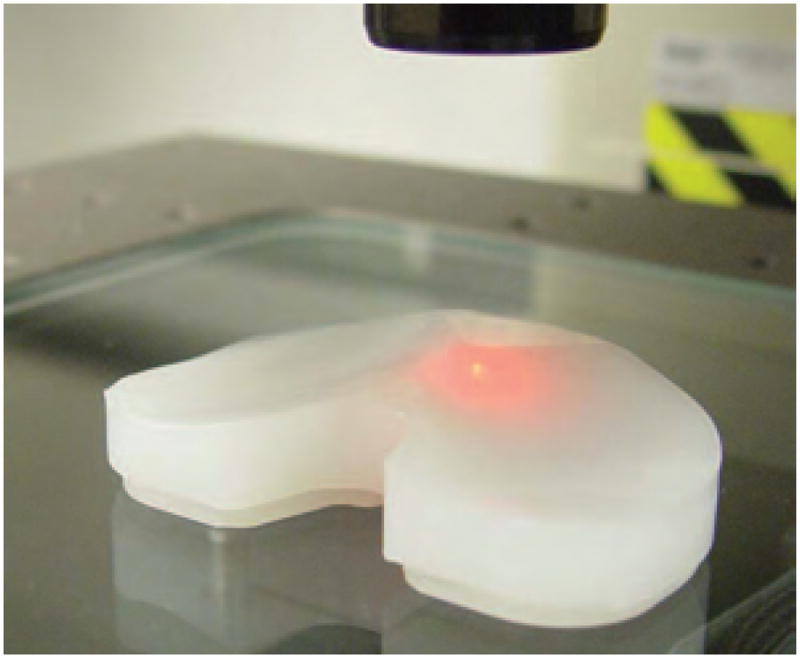
CMM laser scanning of a tibial insert

The mass of the component was measured in a temperature- and humidity-controlled chamber at 25.0±0.02°C with 50.0±0.1% humidity on an AX205 DeltaRange analytic balance (Mettler Toledo, Columbus, OH) with mass resolution of 0.01 mg after passing the sample through a deionizer. Polyethylene was then removed from the articular topside surface of one tibial plateau with an 8mm #5 sweep bent woodcarving gouge (F. Zulauf Messerschmiede und Werkzeugfabrikations AG, Langenthal, Switzerland) while in the chamber. The component was again weighed to find the mass removed. Material was then gouged from the other tibial plateau, and mass was measured. Afterward, components were allowed to acclimate for at least 24 hours to the clean room and digitized with the CMM laser. The scars formed during gouging were mapped by tracing the scar boundary on the CMM under optical light microscopy. The gouged point cloud was rotated and translated to align points outside of the scar with the scan of the insert prior to any testing, similar to that described in literature [24]. A constrained Delaunay triangulation was computed for each scar, and the volume loss was the difference between the volume under the surface prior to testing and volume under the gouged surface. This process of progressive mass removal was performed five times for each component in 10 mg increments.

After each gouging, volume loss was also calculated by autonomous mathematical reconstruction of the original surface. A NexGen design-congruent curve, composed of an anterior radius and a posterior radius whose minima were constrained to be coincident and share a horizontal tangent at their transition point, was fit to points outside the scars for each AP line scan, as in Fig. 4. A least squares fit of this curve was obtained for each AP line scan with a custom written MATLAB active-set constrained optimization [26] to minimize the sum of the square of residuals. Fitted curves were then used to interpolate the initial height of points within the scars, effectively reconstructing original surface. A constrained Delaunay triangulation was computed for each scar, and the volume loss was calculated as the difference between the volumes under the reconstructed original surface and the measured gouged surface. Using the difference between the reconstructed and measured heights at each point in the gouged regions to calculate linear penetration, maps of each component were constructed. The scars defined the regions of interest, and volume changes outside of these were per definition negligible.

Figure 4.

Autonomous mathematical reconstruction least-squares fits a design-congruent curve to the unworn points of an AP line scan (dashed line) to estimate the original surface (solid line) in a worn area (bounded by vertical lines). This allows for calculation of volume lost (gray shaded area). Note that the axes are not to scale and scanned points are denser than depicted.

Six additional NexGen cruciate retaining size Green UHMWPE GUR 1050 tibial inserts, previously worn in level walking gait tests in a four-station knee simulator (Endolab, Rosenheim, Germany) in load-control mode per ISO 14243-1 [27], were also digitized. Inspecting the articular surface for regions where machining marks were still partially present [16,28,29], wear scars were mapped by tracing the scar boundary on the CMM under optical light microscopy. Volume loss was calculated by autonomous mathematical reconstruction. Once volume losses were calculated, testing conditions and total mass lost during simulator testing, measured according to ISO 14243-2 [30], were retrieved from laboratory records. Simulator testing was performed by personnel not part of this study and had ended at least 27 months prior to CMM scanning, during which components had been stored in a temperature-regulated room at 22±1°C.

For both sample groups, gravimetric wear was converted to volume loss assuming the density of polyethylene to be 0.931 mg/mm³ [24,31]. Simple linear regressions of the form

$$y=\alpha +\beta x$$ (2)

were performed to find the slope and intercepts of geometric-to-gravimetric correlations. One-sample independent student t-tests were used to compare the slopes and intercepts to β₀=1 and α₀=0, respectively. For gouged components, paired t-tests compared mass loss to volume loss.

Nine surgically retrieved UHWMPE Miller-Galante II TKR (Zimmer) tibial inserts of two sizes (n_large=5, n_small=4) were also scanned. Implantation times ranged from 4.1 to 30.2 months. Three observers independently scored components for deformation/creep, delamination, polishing and pitting, where the final scores were a product of extent and severity averaged across observers. This study excluded delaminated inserts, postmortem retrievals and inserts with significant edge loading. Scanned inserts were selected from a larger population of retrievals to represent a wide range of total damage scores and patient demographics. Components were reconstructed as before, and volume loss from the articular surface was calculated and mapped. The p-values for linear correlations of volume loss to damage scores were computed.

Results

The convex hemisphere simulation showed that relative volumetric error V_% varied as according to Eq. 3 (R²=1).

$$V_{\%}=\frac{V_I-V_M}{V_I}\approx \frac{C(f)}{{(n-1)}^2}$$ (3)

The relationship of the coefficient C(f) to f in the range of f=0.1 to f=√2 was calculated for diagonals that result in a lower volume error (Fig. 2a) and diagonals that results in an upper volume error (Fig. 2b.) An exponential of a fifth degree polynomial of f, as described by Eqs. 4 and 5, could estimate the upper and lower C(f) values (R²=0.9968 and R²=0.9994, respectively.)

$$C_{\mathit{upper}}(f)\approx e^{5.08f^5-19.61f^4+30.93f^3-26.62f^2+16.21f-7.43}$$ (4)

$$C_{\mathit{lower}}(f)\approx e^{3.18f^5-13.16f^4+22.96f^3-22.47f^2+15.34f-7.38}$$ (5)

The ideal volume of the hemisphere within the limits of the grid can be described by Eq. 6.

$$V_I=G(f)·\pi ·R^3$$ (6)

A fourth order polynomial closely predicted the coefficient G(f) as a function of f (R²=1):

$$G(f)\approx -0.05323f^4+0.04956f^3+0.2888f^2+0.005151f$$ (7)

The number of points per given area defines the point density ρ, which is the in-plane two-dimensional resolution. For the grid size and spacing in this simulation, point density ρ is defined by Eq. 8.

$$\rho ={\left(\frac{n-1}{f·R}\right)}^2$$ (8)

Combining Eqs. 2, 5 and 7, a relationship of volume error V_E to radius of curvature R, resolution ρ and the ratio of the grid length to the curvature f was derived in Eq. 9.

$$V_E=V_I-V_M\approx \frac{C(f)·G(f)·\pi ·R}{f^2\rho }$$ (9)

As seen in Fig. 5, the volume error due to sampling converges as point density increases. For a single tibial insert size, Fig. 5a shows the volume error convergence of a single tibial plateau by sampling a CAD surface and the values predicted by the hemisphere model equation (Eq. 9.) For the same size, Fig. 5b displays the oscillating convergence for the saddle regions on the part. The hemisphere model equation closely predicted the convergence of the volume error for an entire CAD surface, as seen in Fig. 5c. The dependence of volume error on sampling resolution for all sizes of NexGen inserts is shown in Fig. 5d. An XY point spacing of 100x100μm resulted in a sampling error less than 0.75 mm³ for all sizes except one, which had an error of 1.32 mm³.

Figure 5.

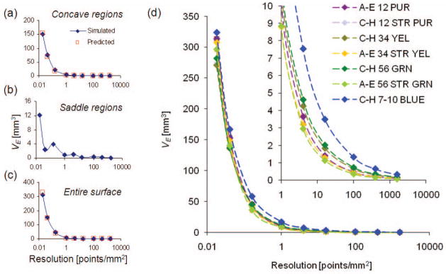
Representative volume error curves for (a) a concave region, (b) a saddle region and (c) the entire surface for hemisphere model predicted values (red squares) and in silico simulated digitization values (blue diamonds). (d) Convergence of sampling volume error at full-scale and the tail region (1–10,000 points/mm²).

The cumulative mass removed from a single tibial plateau ranged from 7.43 mg to 62.48 mg, and wear scars ranged in area from 156 mm² to 698 mm². The volume loss calculated using the component scan prior to any testing correlated strongly to converted mass loss (R²=0.970), as seen in Fig. 6. Volume loss calculated by autonomous mathematical reconstruction also correlated strongly to mass measurements (R²=0.954), as shown in Fig. 6. Table 2 shows that for both of these correlations, the slopes of the regression lines are not significantly different from β=1 and intercepts are not significantly different from α=0. The absolute mean difference (±SD) between volume loss and converted mass loss using the component scan prior to any testing was found to be 3.19±1.77 mm³, while it was found to be 4.72±3.86 mm³ using autonomous reconstruction.

Figure 6.

Relationships of total measured mass loss on a single tibial plateau to volume loss as calculated using the component scan prior to any testing (black dots and solid line) and to volume loss as calculated by autonomous reconstruction (white dots and dashed line).

Table 2.

Linear regressions estimators expressed as mean ± standard error of the mean, and p-values for geometric-to-gravimetric volume loss correlations.

Regression parameters	Volume loss, as calculated compared to initial scan	Volume loss, as calculated by autonomous reconstruction	Volume loss of simulator components
R2	0.970	0.954	0.981
β̂ [mm3/mm3]	0.94± 0.03	1.02± 0.04	1.01± 0.07
p (β=1)	0.054	0.600	0.357
α̂ [mm3]	1.94± 1.30	3.08± 1.77	8.32 ± 0.76
p (α=0)	0.145	0.093	0.0004

Figure 7 compares the visual appearance of the gouged surface of one component to the linear penetration maps obtained using the component scan prior to any testing and reconstruction. Many features can be discerned using both methods, including gouges made at an angle to the AP direction. At the largest wear scar area, some artifacts of reconstruction appear, such as a small furrow in the AP direction in the center of left tibial plateau and a patch of negative penetration in the left posterior region of the right tibial plateau. However, patches of negative penetration also appear in the maps derived from the component scan prior to any testing, most frequently near the intercondylar ridge of the inserts.

Figure 7.

Visual inspections of one gouged component reveal that the corresponding linear penetration maps created using the component scan prior to any testing and autonomous reconstruction show good fidelity of features.

The six NexGen simulator components came from three different knee simulator tests running load-controlled level walking. One component had been used in a wear test for 4 million cycles (Test 1). Three components had been tested for 5 million cycles in a different wear test (Test 2). Two components had been tested in a different test for 5 million cycles (Test 3).

Simulator-tested inserts had wear scars on each tibial plateau with area of 346.94±39.23 mm². Autonomous reconstruction accurately ranked volume loss in order of increasing mass loss. Figure 8 shows that volume loss calculated by autonomous reconstruction had a strong linear correlation to mass loss measured during simulator testing (R²=0.981). As shown in Table 2, the slope of the regression line is not significantly different from β=1, and the intercept is significantly different from α=0.

Figure 8.

Comparison of geometric volume loss as estimated by autonomous reconstruction to total measured mass loss during knee simulator wear tests

Wear maps were created for each measured component. The contours levels in the worn regions showed good qualitative agreement with the shapes of the wear scars, as in Fig. 9. No large areas of severely discontinuous linear penetration values were observed.

Figure 9.

Volume loss maps of the articular surfaces of knee simulator worn components with wear scars outlined in a dashed white line. Shapes next to figure letters correspond to their respective tests as displayed in Fig. 4 (square for Test 1, triangle for Test 2 and diamond for Test 3). Total mass loss for each component is (a) 0.42 mg, (b) 4.76 mg, (c) 5.08 mg, (d) 6.60 mg, (e) 9.46 mg and (f) 19.09 mg.

Total volume loss correlated to months in situ (2.88*months + 7.12 mm³, p= 0.025), which results in wear rates of β_large=39.2±7.2 mm³/year and β_small=15.7±2.7 mm³/year (mean ± SE). Figure 10 shows that for each size, total visual damage scores for the entire surface correlated with total volume loss (p_large=0.001, p_small=0.0137).

Figure 10.

Size correlations of total articular surface volume loss to total articular surface damage scores on nine UHWMPE MGII revision retrieved tibial components.

Discussion

Though many techniques exist to evaluate damage on tibial inserts, each has its own advantages and disadvantages. We have developed a method for surgically retrieved tibial inserts that allows researchers to quantitatively estimate volume loss and its spatial distribution without prior knowledge of the original surface.

Low scanning resolutions and the ability to accurately estimate the original surface of tibial inserts has limited researchers’ capacity to measure low wear volumes. This study found that to reduce the volume error due to digital sampling below 1 mm³, a point spacing of 100x100μm is required. This translated to approximately 400,000 surface points obtained in 18 hours of scanning. Few studies have used a similarly high sampling resolution to analyze volume loss on tibial components [9]. Otherwise, wear on knee-simulator and retrieved tibial components has been reported using in-plane resolutions of 127x127μm [18], 300x300μm [32,33], 500x500μm [16], 750x750μm [24,34,35] and up to 5x5mm [12]. Though these resolutions were used on various designs and sizes of tibial inserts, our work suggests these sampling resolutions could result in sampling volume error of 0.5–2 mm³, 1.25–3.5 mm³, 3–7.5 mm³, 8–15 mm³ and 140–170 mm³, respectively. A recent study using micro-computed tomography analyzed surface deviation on worn tibial inserts with a voxel size of 50μm [36]. Although this provides a higher in-plane resolution, the relative three-dimensional resolution is lower (8000 points/mm³) than the scanning resolution of this study (50,000 point/mm³) because the CMM laser works with a higher depth resolution. Our work with retrieved tibial inserts has revealed that reconstructed CMM lasers scans at 100x100μm maintain some fidelity of surface pitting features, as in Fig. 11.

Figure 11.

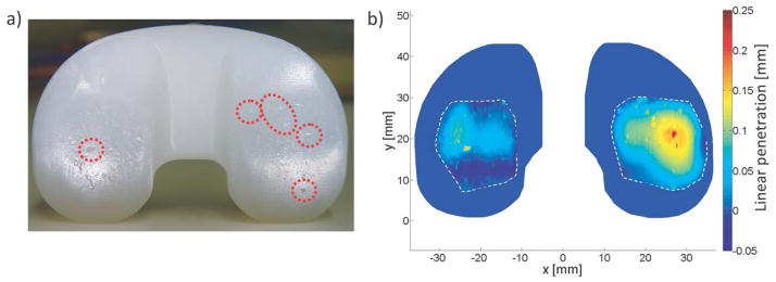
a) A photograph of a surgically retrieved tibial insert shows that macroscopic surface pitting (circled) is also observed in b) a reconstructed penetration map.

Unlike hip replacement retrieval analysis, where the original surface often can be assumed to be spherical, the complex geometry of tibial TKR surfaces makes analysis difficult. Other studies that have attempted to mathematically reconstruct the original surface of tibial inserts have had limited success [12,22], possibly due to lower scanning resolutions and the shapes of reconstructing curves. Our method differs in that a curve congruent to the surface design was fit to unworn regions, instead of polynomials (Seebeck 1997, experimental thesis at Technical University of Hamburg-Harburg, Germany) or non-uniform random b-splines [23]. This study found the volume error associated with autonomous mathematical reconstruction of the surface to be small (less 5 mm³ per tibial plateau) relative to the 10–20 mm³ annual wear rate of UHMWPE [4]. Methods using CAD models and size-matched unused inserts cannot approximate the original surface perfectly due to manufacturing variability [37]. A micro-CT study suggests that a reference geometry averaging three to six unused size-matched inserts can greatly improve accuracy [25], but this multiplies the expense of analyzing retrieved inserts. In our study, autonomous mathematical reconstruction was able to reasonably estimate the original surface for scars as large as 698 mm² (Fig. 7).

Progressive mass removal showed excellent agreement between gravimetric and geometric measurements of volume loss using reconstruction. Volume loss based on insert scans prior to any testing are representative of current in vitro and ideal retrieval methods, where the original unworn surface of the tibial component can be measured. Autonomous reconstruction, which is independent of the availability of unworn inserts, demonstrated similarly accurate results (Fig. 6). Notably, autonomous mathematical reconstruction was able to closely measure the volume loss for volumes less than 20 mm³. The accurate measurement of small wear volumes will be important as cross-linked UHWMPE and other materials reduce the expected wear rate.

Tibial inserts tested in a knee simulator were treated like surgically retrieved inserts for which the mass loss had been precisely measured. The positive intercept between volume loss to mass loss of simulator components was expected, as some volume is lost to deformation and creep of polyethylene during knee simulator wear testing [24]. The intercept of the volume-to-mass correlation on simulator-worn components suggests a creep volume of 8.3 mm³. Interestingly, this agrees with the intercept of the volume-to-time in situ correlation for our group of retrieved components, which suggests a creep volume of 7.1 mm³ at zero months.

Volume loss on revision retrieved components correlated strongly to semi-quantitative visual damage scores based on Hood, et al., 1983 [5], which remains the most common method to analyze retrieved tibial inserts. While our results show close agreement, the differences in volume loss between inserts of different sizes with similar damage scores highlights the need to evaluate retrievals quantitatively.

Some limitations are apparent in our study. The effect of depth accuracy of the CMM was not analyzed, as the error was assumed to be stochastic. We excluded areas of visible edge loading and large deformation from reconstruction, but scars that cover the entire surface may impair mathematical reconstruction. Therefore, CAD models and size-matched unused inserts still have utility in analyzing retrieved tibial inserts. Volume loss due to wear and volume loss due to creep cannot be distinguished by any geometric technique alone. However, in combination with measured mass loss, creep can be estimated [24]. The accuracy and precision of gravimetric measurements is limited by fluid absorption and static charging of the polyethylene [38]. Although load-soak controls attempt to correct for fluid absorption, the smaller loading area without relative motion cannot reproduce the exact fluid absorption experienced by articulating inserts and therefore leads to underestimates of mass loss. Additionally, gravimetric measurements cannot distinguish articular topside wear from inferior backside wear. Thus, backside wear may also confound our calculation of volume loss due to creep. Methods of geometrically estimating backside wear exist [9,11], and we believe that autonomous mathematical reconstruction could be extended to the backside based on previous profile measurements of unworn inserts [39]. Our study investigated volume error and autonomous mathematical reconstruction using only two implant designs; however, we believe that the method for reconstruction can be generalized to different designs.

Though we obtained a point cloud representation of the surface with a CMM routine, autonomous reconstruction can be applied to surfaces of diverse geometries digitized by other methods. The technique produces many different wear metrics: volume loss on each tibial plateau, solid centroid of each wear scar, area of wear scars, maximum linear penetration on each tibial plateau, locations of maximum linear penetrations and a wear map of the surface. These metrics will provide researchers with a more complete understanding of wear on UHWMPE tibial liners.

Conclusion

With a high sampling resolution, geometric measurement of volume loss through autonomous reconstruction correlates strongly to gravimetric measurements, from which one could hypothesize that autonomous reconstruction can be used as a powerful tool for geometric wear analysis of retrieved tibial inserts.

References

- 1.Kurtz S, Ong K, Lau E, Mowat F, Halpern M. Projections of primary and revision hip and knee arthroplasty in the United States from 2005 to 2030. J Bone Joint Surg Am. 2007;89 (4):780–785. doi: 10.2106/JBJS.F.00222. [DOI] [PubMed] [Google Scholar]
- 2.Crowninshield RD, Rosenberg AG, Sporer SM. Changing demographics of patients with total joint replacement. Clin Orthop Relat Res. 2006;443:266–272. doi: 10.1097/01.blo.0000188066.01833.4f. [DOI] [PubMed] [Google Scholar]
- 3.Naudie DD, Ammeen DJ, Engh GA, Rorabeck CH. Wear and osteolysis around total knee arthroplasty. J Am Acad Orthop Surg. 2007;15 (1):53–64. doi: 10.5435/00124635-200701000-00006. [DOI] [PubMed] [Google Scholar]
- 4.Kaddick C, Catelas I, Pennekamp PH, Wimmer MA. Implant wear and aseptic loosening - an overview. Orthopade. 2009;38 (8):690–697. doi: 10.1007/s00132-009-1431-9. [DOI] [PubMed] [Google Scholar]
- 5.Hood RW, Wright TM, Burstein AH. Retrieval analysis of total knee prostheses: a method and its application to 48 total condylar prostheses. J Biomed Mater Res. 1983;17:829–842. doi: 10.1002/jbm.820170510. [DOI] [PubMed] [Google Scholar]
- 6.Blunn GW, Joshi AB, Minns RJ, Lidgren L, Lilley P, Ryd L, Engelbrecht E, Walker PS. Wear in retrieved condylar knee arthroplasties. A comparison of wear in different designs of 280 retrieved condylar knee prostheses. J Arthroplasty. 1997;12 (3):281–290. doi: 10.1016/s0883-5403(97)90024-3. [DOI] [PubMed] [Google Scholar]
- 7.Lavernia CJ, Sierra RJ, Hungerford DS, Krackow K. Activity level and wear in total knee arthroplasty: a study of autopsy retrieved specimens. J Arthroplasty. 2001;16 (4):446–453. doi: 10.1054/arth.2001.23509. [DOI] [PubMed] [Google Scholar]
- 8.Berzins A, Jacobs JJ, Berger R, Ed C, Natarajan R, Andriacchi T, Galante JO. Surface damage in machined ram-extruded and net-shape molded retrieved polyethylene tibial inserts of total knee replacements. J Bone Joint Surg Am. 2002;84-A(9):1534–1540. doi: 10.2106/00004623-200209000-00005. [DOI] [PubMed] [Google Scholar]
- 9.Conditt MA, Thompson MT, Usrey MM, Ismaily SK, Noble PC. Backside wear of polyethylene tibial inserts: mechanism and magnitude of material loss. J Bone Joint Surg Am. 2005;87 (2):326–331. doi: 10.2106/JBJS.C.01308. [DOI] [PubMed] [Google Scholar]
- 10.Currier JH, Bill MA, Mayor MB. Analysis of wear asymmetry in a series of 94 retrieved polyethylene tibial bearings. J Biomech. 2005;38 (2):367–375. doi: 10.1016/j.jbiomech.2004.02.016. [DOI] [PubMed] [Google Scholar]
- 11.Crowninshield RD, Wimmer MA, Jacobs JJ, Rosenberg AG. Clinical performance of contemporary tibial polyethylene components. J Arthroplasty. 2006;21 (5):754–761. doi: 10.1016/j.arth.2005.10.012. [DOI] [PubMed] [Google Scholar]
- 12.Kop AM, Swarts E. Quantification of polyethylene degradation in mobile bearing knees: a retrieval analysis of the Anterior-Posterior-Glide (APG) and Rotating Platform (RP) Low Contact Stress (LCS) knee. Acta Orthop. 2007;78(3):364–370. doi: 10.1080/17453670710013942. [DOI] [PubMed] [Google Scholar]
- 13.Garcia RM, Kraay MJ, Messerschmitt PJ, Goldberg VM, Rimnac CM. Analysis of retrieved ultra-high-molecular-weight polyethylene tibial components from rotating-platform total knee arthroplasty. J Arthroplasty. 2009;24 (1):131–138. doi: 10.1016/j.arth.2008.01.003. [DOI] [PubMed] [Google Scholar]
- 14.Orozco DA, Wimmer MA. Pictorial information of TKA wear scars provides information beyond the intrinsic geometrical factors. J Biomech. 2006;39 (1):S120. [Google Scholar]
- 15.Grochowsky JC, Alaways LW, Siskey R, Most E, Kurtz SM. Digital photogrammetry for quantitative wear analysis of retrieved TKA components. J Biomed Mater Res B Appl Biomater. 2006;79 (2):263–7. doi: 10.1002/jbm.b.30537. [DOI] [PubMed] [Google Scholar]
- 16.Harman MK, Desjardins J, Benson L, Banks SA, Laberge M, Hodge WA. Comparison of polyethylene tibial insert damage from in vivo function and in vitro wear simulation. J Orthop Res. 2009;27(4):540–548. doi: 10.1002/jor.20743. [DOI] [PubMed] [Google Scholar]
- 17.Plante-Bordeneuve P, Freeman MA. Tibial high-density polyethylene wear in conforming tibiofemoral prostheses. J Bone Joint Surg Br. 1993;75(4):630–636. doi: 10.1302/0301-620X.75B4.8331121. [DOI] [PubMed] [Google Scholar]
- 18.Benjamin J, Szivek J, Dersam G, Persselin S, Johnson R. Linear and volumetric wear of tibial inserts in posterior cruciate-retaining knee arthroplasties. Clin Ortho Relat Res. 2001;392:131–138. doi: 10.1097/00003086-200111000-00016. [DOI] [PubMed] [Google Scholar]
- 19.Ashraf T, Newman JH, Desai VV, Beard D, Nevelos JE. Polyethylene wear in a non-congruous unicompartmental knee replacement: a retrieval analysis. Knee. 2004;11:177–181. doi: 10.1016/j.knee.2004.03.004. [DOI] [PubMed] [Google Scholar]
- 20.Price AJ, Short A, Kellett C, Beard D, Gill H, Pandit H, Dodd CAF, Murray DW. Ten-year in vivo wear measurement of a fully congruent mobile bearing unicompartmental knee arthroplasty. J Bone Joint Surg Br. 2005;87-B(11):1493–1497. doi: 10.1302/0301-620X.87B11.16325. [DOI] [PubMed] [Google Scholar]
- 21.Gill HS, Waite JC, Short A, Kellett CF, Price AJ, Murray DW. In vivo measurement of volumetric wear of a total knee replacement. Knee. 2006;13 (4):312–317. doi: 10.1016/j.knee.2006.04.001. [DOI] [PubMed] [Google Scholar]
- 22.Kendrick BJ, Longino D, Pandit H, Svard U, Gill HS, Dodd CA, Murray DW, Price AJ. Polyethylene wear in Oxford unicompartmental knee replacement: a retrieval study of 47 bearings. J Bone Joint Surg Br. 2010;92 (3):367–373. doi: 10.1302/0301-620X.92B3.22491. [DOI] [PubMed] [Google Scholar]
- 23.Blunt LA, Bills PJ, Jiang XQ, Chakrabarty G. Improvement in the assessment of wear of total knee replacements using coordinate-measuring machine techniques. Proc Inst Mech Eng H. 2008;222 (3):309–318. doi: 10.1243/09544119JEIM289. [DOI] [PubMed] [Google Scholar]
- 24.Muratoglu OK, Perinchief RS, Bragdon CR, O’Connor DO, Konrad R, Harris WH. Metrology to quantify wear and creep of polyethylene tibial knee inserts. Clin Orthop Relat Res. 2003;410:155–164. doi: 10.1097/01.blo.0000063604.67412.04. [DOI] [PubMed] [Google Scholar]
- 25.Teeter MG, Naudie DD, Milner JS, Holdsworth DW. Determination of reference geometry for polyethylene tibial insert wear analysis. J Arthroplasty. 2011;26 (3):497–503. doi: 10.1016/j.arth.2010.01.096. [DOI] [PubMed] [Google Scholar]
- 26.Powell MJD. The Convergence of Variable Metric Methods For Nonlinearly Constrained Optimization Calculations. In: Mangasarian OL, Meyer RR, Robinson SM, editors. Nonlinear Programming. Vol. 3. Academic Press; 1978. [Google Scholar]
- 27.ISO International Standard 14243-1, Implants for surgery – Wear of total knee-joint prostheses – Part 1: Loading and displacement parameters for wear-testing machines with load control and corresponding environmental conditions for test, 2002.
- 28.McKellop H, Campbell P, Park SH, Schmalzried TP, Grigoris P, Amstutz HC, Sarmiento A. The origin of submicron polyethylene wear debris in total hip arthroplasty. Clin Orthop. 1995;311:3–20. [PubMed] [Google Scholar]
- 29.Wimmer MA, Paul P, Haman J, Schwenke T, Rosenberg AG, Jacobs JJ. Differences in damage between revision and postmortem retrieved TKA implants. Transactions of the 51st Annual Meeting of the Orthopaedic Research Society; 2005. poster #1204. [Google Scholar]
- 30.ISO International Standard 14243-2. Implants for surgery—wear of total knee-joint prostheses. Part 2. Methods of measurement. 2000 [Google Scholar]
- 31.Kurtz SM. A primer on UHWMPE. In: Kurtz SM, editor. UHWMPE Biomaterials Handbook. 2. Boston: Academic Press; 2009. pp. 1–6. [Google Scholar]
- 32.Affatato S, Spinelli M, Zavalloni M, Carmignato S, Lopomo N, Marcacci M, Viceconti M. Unicompartmental knee prostheses: in vitro wear assessment of the menisci tibial insert after two different fixation methods. Phys Med Biol. 2008;53:5357–5369. doi: 10.1088/0031-9155/53/19/006. [DOI] [PubMed] [Google Scholar]
- 33.Spinelli M, Carmignato S, Affatato S, Viceconti M. CMM-based procedure for polyethylene non-congruous unicompartmental knee prosthesis wear assessment. Wear. 2009;267:753–756. [Google Scholar]
- 34.Muratoglu OK, Bragdon CR, Jasty M, O’Connor DO, Von Knoch RS, Harris WH. Knee-simulator testing of conventional and cross-linked polyethylene tibial inserts. J Arthroplasty. 2004;19 (7):887–897. doi: 10.1016/j.arth.2004.03.019. [DOI] [PubMed] [Google Scholar]
- 35.Muratoglu OK, Rubash HE, Bragdon CR, Burroughs BR, Huang A, Harris WH. Simulated normal gait wear testing of a highly cross-linked polyethylene tibial insert. J Arthroplasty. 2007;22 (3):435–444. doi: 10.1016/j.arth.2006.07.014. [DOI] [PubMed] [Google Scholar]
- 36.Teeter MG, Naudie DDR, McErlain DD, Brandt JM, Yuan X, MacDonald SJ, Holdsworth DW. In vitro quantification of wear in tibial inserts using microcomputed tomography. Clin Orthop Relat Res. 2011;469:107–112. doi: 10.1007/s11999-010-1490-6. [DOI] [PMC free article] [PubMed] [Google Scholar]
- 37.Knowlton CB, Hansen G, Orozco D, Laurent MP, Wimmer MA. Geometric measurement of wear in tibial inserts through an autonomous reconstruction of the original surface. Proceedings of the ASME 2011 Summer Bioengineering Conference; 22–25 June 2011; poster #53754. [Google Scholar]
- 38.Schwenke T, Kaddick C, Schneider E, Wimmer MA. Fluid composition impacts standardized testing protocols in ultrahigh molecular weight polyethylene knee wear testing. Proc Inst Mech Eng H. 2005;219:457–464. doi: 10.1243/095441105X34392. [DOI] [PubMed] [Google Scholar]
- 39.Surace MF, Berzins A, Urban RM, Jacobs JJ, Berger RA, Natarajan RN, Andriacchi TP, Galante JO. Backsurface wear and deformation in polyethylene tibial inserts retrieved postmortem. Clin Orthop Relat Res. 2002;404:14–23. doi: 10.1097/00003086-200211000-00004. [DOI] [PubMed] [Google Scholar]