Spatial Heterogeneity of Cortical Receptive Fields and Its Impact on Multisensory Interactions

Abstract

Investigations of multisensory processing at the level of the single neuron have illustrated the importance of the spatial and temporal relationship of the paired stimuli and their relative effectiveness in determining the product of the resultant interaction. Although these principles provide a good first-order description of the interactive process, they were derived by treating space, time, and effectiveness as independent factors. In the anterior ectosylvian sulcus (AES) of the cat, previous work hinted that the spatial receptive field (SRF) architecture of multisensory neurons might play an important role in multisensory processing due to differences in the vigor of responses to identical stimuli placed at different locations within the SRF. In this study the impact of SRF architecture on cortical multisensory processing was investigated using semichronic single-unit electrophysiological experiments targeting a multisensory domain of the cat AES. The visual and auditory SRFs of AES multisensory neurons exhibited striking response heterogeneity, with SRF architecture appearing to play a major role in the multisensory interactions. The deterministic role of SRF architecture was tightly coupled to the manner in which stimulus location modulated the responsiveness of the neuron. Thus multisensory stimulus combinations at weakly effective locations within the SRF resulted in large (often superadditive) response enhancements, whereas combinations at more effective spatial locations resulted in smaller (additive/subadditive) interactions. These results provide important insights into the spatial organization and processing capabilities of cortical multisensory neurons, features that may provide important clues as to the functional roles played by this area in spatially directed perceptual processes.

INTRODUCTION

The natural world is comprised of a vast array of sensory cues that can occur simultaneously and in association with a variety of different events. The complexities of these events pose a significant challenge to the CNS. Peripheral sensory organs are designed to collect a single form of environmental energy, but the overall goal of the CNS is to build a composite percept of the world. As a likely solution to this problem, the brain has dedicated regions that are specialized for the processing of convergent inputs from multiple sensory modalities (Stein and Meredith 1993). Although such convergence takes place at virtually all levels of the neuraxis, multisensory circuits within the cerebral cortex are likely to play an important role in the creation of our perceptual gestalt. Nonetheless, despite its potential importance in shaping our perceptions, our knowledge of multisensory cortical processing remains quite limited.

There are a number of candidate cortical areas for examining the neural substrates of multisensory processing (Calvert et al. 2004; Ghazanfar and Schroeder 2006). In the nonhuman primate, physiological recordings have revealed multisensory interactions in the superior temporal sulcus (STS; see Barra-clough et al. 2005; Schroeder and Foxe 2002), intraparietal sulcus (areas VIP and LIP; see Avillac et al. 2005; Duhamel et al. 1998; Schlack et al. 2005; Schroeder and Foxe 2002), frontal cortical domains (see Romanski 2007; Sugihara et al. 2006), and increasingly even in areas traditionally considered unisensory (e.g., see Brosch et al. 2005; Ghazanfar et al. 2005; Kayser et al. 2005; Lakatos et al. 2007; Schroeder et al. 2001). In addition, a growing body of human neuroimaging data is beginning to elucidate the cortical bases for multisensory interactions (e.g., for recent reviews see Driver and Noesselt 2008; Ghazanfar and Schroeder 2006).

In the cat, the principal cortical site for the study of multisensory processing has been the cortex surrounding the anterior ectosylvian sulcus (AES). Although the functional role of the AES remains unresolved, the substantial convergence of visual, auditory, and somatosensory inputs suggests that this area plays an important role in the perceptual synthesis of multisensory information. Thus in addition to being divided into three distinct unisensory domains [i.e., the anterior ectosylvian visual area (AEV) (Benedek et al. 1988; Mucke et al. 1982; Norita et al. 1986); the fourth somatosensory cortex (SIV) (Clemo and Stein 1982, 1983, 1984); and the auditory field AES (FAES) (Clarey and Irvine 1986, 1990a,b)], the AES also contains a substantial population of multisensory neurons. These multisensory neurons are clustered at the borders between the major unisensory domains (Wallace et al. 2006; but see Jiang et al. 1994a,b) and reflect the modalities represented in the neighboring domains (e.g., visual–auditory neurons are of highest incidence at the border between AEV and FAES). Such an organizational scheme has been suggested to be a general plan for cortical parcellation (Beauchamp et al. 2004; Brett-Green et al. 2003; Wallace et al. 2004).

Rather than serving as passive conduits for multisensory information, multisensory AES neurons have been shown to actively integrate their different sensory inputs. This integration gives rise to responses that typically differ substantially from the component unisensory responses and that often differ significantly from the predicted summation of these responses (Stein and Wallace 1996; Wallace et al. 1992). As has been well established for multisensory neurons in other brain structures [most notably the superior colliculus (SC) of the midbrain], the nature of the integrated multisensory responses seen in these neurons is critically dependent not only on the spatial (Meredith and Stein 1986a) and temporal (Meredith et al. 1987) relationships of the stimuli that are combined, but also on their relative effectiveness (Meredith and Stein 1986b). However, despite the utility of these principles as general operational guidelines for understanding the combinatorial properties of multisensory circuits, they provide only limited predictive insight into the product of a specific multisensory combination in any given neuron. For example, whereas some multisensory neurons have been shown to exhibit large superadditive response enhancements when subjected to spatially and temporally coincident pairings of weakly effective stimuli, others respond to similar pairings with only modest subadditive enhancements (Perrault Jr et al. 2003; Stanford et al. 2005, 2007). Recent work has helped elucidate some of the reasons for this variability by demonstrating that SC multisensory neurons can be divided into several operational categories, with the neuron’s categorization being highly correlated with the size of its dynamic response range (Perrault Jr et al. 2005). Thus neurons exhibiting superadditive interactions were found to have restricted dynamic response ranges, whereas those showing additive and/or subadditive interactions were found to have much larger dynamic ranges. Such a finding reinforces the preeminent role of stimulus effectiveness in determining the resultant interaction and also suggests that the integrated responses of multisensory neurons may be highly dependent on intrinsic neuronal characteristics.

One intrinsic factor whose role in multisensory interactions has not been explored is receptive field architecture. Although conventional representations of receptive fields simply delimit an area of space in which excitatory responses can be evoked, numerous prior studies of multisensory neurons have shown that strikingly different responses can be generated to identical stimuli positioned at different locations within the classical receptive field (King and Palmer 1985; Meredith et al. 1983, 1986a, 1996; Wallace et al. 1992, 1997, 1998). Although noted, the impact of such heterogeneity on multisensory interactions has not been systematically investigated. Multisensory neurons in the cat AES provide an excellent substrate within which to investigate this issue, both because their receptive fields are quite large and because it has been suggested that these neurons encode spatial information via differential responses as a function of stimulus location (Benedek et al. 2004; Eordegh et al. 2005; Furukawa and Middlebrooks 2002; Middlebrooks et al. 1984, 1998; Nagy et al. 2003a,b; Xu et al. 1999). Consequently, in the current study we set out to begin to characterize the spatial heterogeneity of receptive fields in multisensory AES neurons and, more important, to examine how this architecture contributes to the multisensory interactions that characterize these neurons. This work is predicated on a provocative new theoretical framework postulating that space contributes to multisensory interactions in large measure through its impact on neuronal responsiveness.

METHODS

General procedures

Experiments were conducted in adult cats (n = 4) raised under standard housing conditions. All experiments were done in an anesthetized and paralyzed semichronic preparation and consisted of single-unit extracellular recordings from neurons in the cortex of the anterior ectosylvian sulcus (AES). Experiments were run on a weekly basis on each animal, with the total number of experiments per animal ranging from 10 to 27. All surgical and recording procedures were performed in compliance with the Guide for the Care and Use of Laboratory Animals (National Institutes of Health publication number 91-3207) at Vanderbilt University Medical Center, which is accredited by the American Association for Accreditation of Laboratory Animal Care.

Implantation and recording procedures

Presurgical anesthesia was induced with ketamine hydrochloride [20 mg/kg, administered intramuscularly (im)] and acepromazine maleate (0.04 mg/kg im). For the implantation of the recording chamber over AES, animals were transported to a central surgical suite, where they were intubated and artificially respired. A stable plane of surgical anesthesia was achieved using inhalation isoflurane (1.0–3.0%). Body temperature, expiratory CO₂, blood pressure, and heart rate were continuously monitored (VSM7, Vetspecs), recorded, and maintained within bounds consistent with a deep and stable plane of anesthesia. A craniotomy was made to allow direct access to the cortical surface surrounding the AES. A stainless steel recording chamber and head holder were attached to the skull using stainless steel bone screws and orthopedic cement. Such a design allowed the animal to be maintained in a recumbent position during recordings without obstructing the face and ears. Preoperative and postoperative care (i.e., analgesics and antibiotics) were administered in close consultation with veterinary staff. A minimum of 1-wk recovery was allowed prior to the first recording session.

For recording experiments, anesthesia was induced with a bolus of ketamine (20 mg/kg im) and acepromazine maleate (0.04 mg/kg im) and maintained throughout the procedure with a constant rate infusion of ketamine [5 mg·kg⁻¹ · h⁻¹, administered intravenously (iv)] delivered through a cannula placed in the saphenous vein. Although the impact of ketamine anesthesia on multisensory processes has been a subject of debate (Populin et al. 2002, 2005; Stanford et al. 2005, 2007), we have seen little difference in the receptive fields or multisensory integrative capacity of neurons in a comparison between the ketamine-anesthetized and awake preparations (Wallace et al. 1994, 1998). The animal was then comfortably supported in the recumbent position without any wounds or pressure points via the head-holding system. To prevent ocular drift, animals were paralyzed with pancuronium bromide (0.1 mg·kg⁻¹ ·h⁻¹, iv), and artificially respired for the duration of the recording. On completion of the experiment animals were subcutaneously given an additional 60–100 ml of lactated Ringer solution to facilitate recovery. Parylene-insulated tungsten microelectrodes (Z = 1–3 MΩ) were advanced into the AES using an electronically controlled mechanical microdrive. Single-unit neural activity (isolation criterion: 3:1 signal to noise) was recorded, amplified, and routed to an oscilloscope, audio monitor, and computer for performing on- and off-line analyses.

Search strategy

Initial recording experiments targeted the center of each sensory representation. On establishment of these core areas subsequent penetrations targeted the border regions to increase the probability of encountering units responsive to multiple sensory inputs (Fig. 1D). In an effort to identify sensory-responsive neurons within the AES and to determine the neuronal selectivity that will be used to tailor later quantitative testing (see following text), a battery of search stimuli was used (for more detail see Perrault Jr et al. 2003; Wallace et al. 2006). Visual search stimuli consisted of moving bars of light projected onto a translucent tangent screen. Stimulus size, intensity, orientation, speed, and direction of movement were varied to determine gross receptive field borders (see following text) and to obtain a coarse tuning profile for the neuron under study, consequently delimiting the stimulus parameters that were used for quantitative testing. Auditory search stimuli consisted of clicks, hisses, whistles, claps, and broadband noise bursts that could be delivered at all locations around the animal. Because of the ease in relating between the coordinate systems of visual and auditory space, visual–auditory multisensory AES neurons were the exclusive focus of the current study.

Fig. 1.

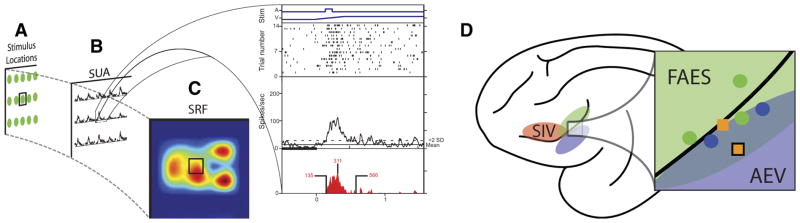
Construction of spatial receptive field (SRF) plots and location of recorded neurons. A: an example array of spatial locations (green dots) in which visual, auditory, and paired visual–auditory stimuli are presented to a multisensory neuron. B: the single-unit activity (SUA) at each of the tested locations is represented as stimulus-evoked spike density functions. The expansion box shows the raw data for a multisensory response at a single location and is composed of 4 panels. The top panel shows the visual (V: movement depicted by ramp) and auditory (A: square wave) stimulus onset and offset times. The 2nd panel shows a raster plot of the neuronal response, with each dot representing an action potential and each row representing a single trial. The 3rd panel shows a collapsed spike density function, with the dotted line representing the response level 2SDs above baseline (i.e., the response criterion). The bottom panel shows only the statistically defined evoked response (red shading) and illustrates various aspects of the temporal dynamics (onset, peak, and offset) of the evoked response. C: the evoked response at each location is then normalized to the greatest elicited response across conditions, with the warmth of the color representing the magnitude of the response. D: shown on the schematic view of lateral surface of the cat brain is the location of electrode penetrations through anterior ectosylvian sulcus (AES) cortex for one animal. Colored shading highlights the 3 unisensory subdivisions of the AES cortex: 4th somatosensory cortex (SIV, red), auditory field AES (FAES, green), and anterior ectosylvian visual area (AEV, blue). The circles represent penetrations in which only unisensory units were isolated, with the color representing the effective modality (visual: blue; auditory: green). Squares represent penetrations in which multisensory neurons (visual–auditory) were isolated and recorded; the black outlined square represents the location of the penetration in which the unit in Fig. 4 was recorded. Note that multisensory units were isolated on penetrations located on the border between FAES and AEV. Due to the complex geometry of the AES, only penetrations in which the approach angle was equivalent are shown in this figure.

Stimulus presentation

Following unit isolation, the general borders of the visual and auditory receptive fields of the neuron were determined using the search stimuli described earlier. As in previous descriptions of AES multisensory neurons (Jiang et al. 1994a; Wallace et al. 1992), the borders of these receptive fields were found to be highly overlapping and this region of overlap was the focus of the spatial receptive field and multisensory interactive analyses. We use the term spatial receptive field (SRF) here to differentiate the higher-resolution mapping analyses from the simple determination of receptive field borders. To best characterize the influence of SRF organization on multisensory interactions, a single stimulus intensity for each of the effective modalities was chosen that optimized the probability of generating response enhancements (Meredith and Stein 1986b; Perrault Jr et al. 2003). For these spatial analyses, only stimulus location was changed and all other stimulus parameters were identical. An array of stimulus locations was chosen with a typical spacing of 10° in both azimuth and elevation to sample from a variety of locations within the region of overlap of the neuron’s visual and auditory receptive fields (Fig. 1). As an example, if the area of receptive field overlap was 40 × 40°, the neuron would be tested at 16 locations and at additional locations immediately outside of the area of overlap (i.e., 10° outside of the overlap border). All locations were tested with both unisensory (i.e., visual alone, auditory alone) and spatially coincident multisensory (i.e., visual–auditory) stimuli (note that only spatially coincident pairings were used in this study).

For quantitative tests, visual stimuli were presented monocularly to the eye contralateral to the recording electrode (the ipsilateral eye was covered with an opaque contact lens). Visual stimuli consisted of a moving bar of light (0.11–13.0 cd/m² on a background luminance of 0.10 cd/m²) projected onto a translucent tangent screen (positioned 1 m from the animal’s eyes). Visual stimulus effectiveness was typically manipulated by changing either the direction or speed of movement (70–120°/s) or the physical dimensions of the bar. To avoid confounding the analyses, the amplitude of movement was always 10°, with the visual stimulus location on the SRF plots corresponding to the midpoint of the stimulus sweep. Auditory stimuli were delivered through a freely positionable speaker that was affixed to the tangent screen immediately adjacent to the corresponding visual stimulus location (i.e., spatially coincident). Auditory stimuli consisted of 50-ms-duration broadband (20 Hz to 20 kHz) noise bursts ranging in intensity from 50.6 to 70.0 dB sound pressure level (SPL) on a background of 45 dB SPL (A-weighted). Stimulus conditions [e.g., visual (V), auditory (A), multisensory (VA)] were randomly interleaved until a minimum of 15 trials were collected for each stimulus condition. Consecutive stimulus presentations were separated by no less than 6 s to avoid response habituation. Complete characterization of the neuron’s spatial response and multisensory interactive profiles took between 3 and 3.5 hours.

Data acquisition and analysis

A custom-built PC-based real-time data acquisition system controlled the structure of the trials, the timing of the presented stimuli, and recorded spike data (100 kHz). Analysis of the data was performed off-line using customized scripts in the MATLAB (The MathWorks, Natick, MA) programming environment.

Neuronal responses were characterized through the construction of peristimulus time histograms (PSTHs) and collapsed spike density functions (SDFs). The SDFs were created by convolving the spike train from each trial for a given condition and location with a function resembling a postsynaptic potential specified by τ_g, the time constant for the growth phase, and τ_d, the time constant for the decay according to the following formula: R(t) = [1 −exp(−t/τ_g)] × exp(−t/τ_d) based on physiological data from excitatory synapses, where τ_g was set to 1 ms and τ_d to 20 ms (Kim and Connors 1993; Mason et al. 1991; Sato and Schall 2001; Sayer et al. 1990). Baselines for each SDF were calculated as the mean firing rate during the 1,500 ms immediately preceding stimulus onset. The collapsed SDFs were then set at a threshold, 2SD above their respective baselines to delimit the stimulus-evoked responses. After stimulus onset the time at which the SDF crosses above the 2SD line was noted as the response onset. Response offset was the time at which the SDF fell below the 2SD line and stayed below this line for ≥30 ms. Response duration was defined as the time interval between response onset and response offset. Mean stimulus-evoked response was calculated as the average number of spikes elicited per trial during the defined response duration interval. Single units that failed to demonstrate a significant stimulus-evoked response lasting ≥30 ms in at least one modality were removed from further consideration. For a subset of the neurons examined for the SRF analyses, the spatiotemporal receptive field (STRF) was also constructed by plotting locations along one plane of the investigated field (azimuth or elevation) on the y-axis and the corresponding SDFs along the x-axis. Responses were aligned to the earliest stimulus onset and the SDFs were then interpolated in two dimensions by the method of cubic splines.

Multisensory interactive analyses

Two measures were used to quantify the multisensory interaction at each tested spatial location. The first of these, the interactive index, represents the relative change in a neuron’s response to the multisensory condition when compared with the best unisensory response. The interactive index is calculated using the formula: I = [(M − U)/U] × 100, where I is the multisensory interactive index, M is the response to the multisensory stimulus, and U is the response to the most effective unisensory stimulus (Meredith et al. 1983, 1986b). Statistical comparisons between the mean stimulus-evoked responses of the multisensory condition and the best unisensory condition were done using a two-tailed paired Student’s t-test. The second measure used is mean statistical contrast or multisensory contrast. This metric evaluates the multisensory response as a function of the response predicted by the addition of the two unisensory responses. Multisensory contrast is calculated using the formula: Σ [(SA − A) − (V − VA)]/n, where SA is spontaneous activity, A is auditory response, V is visual response, VA is multisensory response, and n is number of trials. The model assumes independence between the visual and auditory inputs and uses additive factors logic to distinguish between subadditive (contrast <0), additive (contrast = 0), and superadditive (contrast >0) modes of response (Perrault Jr et al. 2003, 2005; Stanford et al. 2005, 2007). Significant differences from a contrast value of zero were determined by means of a t-test.

Spatial receptive field analyses

For each neuron, the mean stimulus-evoked firing rates (Fig. 1B, expanded) were normalized with the highest stimulus-evoked response recorded from all tested conditions and locations, producing a response continuum ranging from 0.0 to 1.0, with 0.0 being no measurable response and 1.0 being the maximum evoked sensory response. When arrayed in a matrix such that the relative positions of these firing rates within the matrix reflected stimulus location, these values revealed the SRF organization for the visual, auditory, predicted multisensory (linear addition of the visual and auditory SRFs), and actual multisensory conditions for the region of receptive field overlap. To aid visualization, this SRF structure was then interpolated using the method of cubic splines (Fig. 1C). To examine the response heterogeneity inherent to unisensory and multisensory SRFs across the population of AES multisensory neurons, the SRFs were converted into their polar coordinate equivalents using the method of vector averaging. The origin of the polar plot is the geometric center of the area investigated. The receptive field is then divided into eight equal size wedges, with the vector magnitude of each wedge representing the magnitude of the sensory-evoked response normalized across conditions for each location. Population plots (Fig. 2C) were created by averaging individual normalized responses across corresponding wedges. The creation of these polar coordinate equivalents not only allows an assessment of the potential spatial biases that may be contained in the SRFs of AES neurons, but also allows the data to be collapsed into a single metric that shows how the population of recorded AES neurons represents space in their mean firing rates.

Fig. 2.

Examples of response heterogeneity in the SRFs of cortical multisensory neurons. A: the visual, auditory, and multisensory SRFs for the region of receptive field overlap in an AES neuron (SRFs constructed as detailed in Fig. 1). Each of the 3 representations has been normalized to the greatest evoked response, with the pseudocolor plots showing the relative activity scaled to this maxima. Below the SRFs are polar plots in which the center of the plot is the geometric center of the tested area of overlap. The magnitude of each wedge is proportional to the evoked response in that region of the receptive field, normalized across conditions (N, nasal; T, temporal; S, superior; I, inferior). B: an example of SRF and polar plots for a second AES multisensory neuron. Note in this example the substantial disparity between the visual and auditory SRFs. C: polar plot representations (grand mean) for the population of AES multisensory neurons. D: the distribution of the population of AES neurons plotted as a function of the Cartesian distance separating the location of the maximal visual and auditory responses. Note that the majority of neurons have a relatively close correspondence (i.e., <20°).

Analysis of inverse effectiveness

In an effort to relate the spatial heterogeneity of AES SRFs to the multisensory product, we selected those interactions in which a significant response enhancement (as defined earlier) was generated and pooled these across neurons to examine the relationship between stimulus effectiveness and the resultant interaction. This analysis was predicated on the idea that the role of space in multisensory interactions may be best revealed by examining its impact on the vigor of the sensory responses at various locations. As highlighted earlier, due to the response heterogeneity of AES SRFs, it was necessary to normalize stimulus-evoked sensory responses within each modality (as described earlier). The multisensory interactive index was then plotted against each of the normalized unisensory stimulus-evoked responses. In addition, the normalized unisensory responses were also categorized into three discrete bins, reflecting the magnitude of their responses: low (0–0.33), medium (0.34–0.66), and high (0.67–1.00). Statistically significant multisensory interactions were then pooled and averaged as a function of the paired unisensory responses (e.g., low–low, low–high, etc.).

RESULTS

Cortical multisensory neurons exhibit marked response heterogeneities within their spatial receptive fields (SRFs)

In all, 97 sensory responsive neurons were isolated in electrode penetrations that targeted the multisensory domain between AEV and FAES of AES cortex in four adult cats. Of these, 33% (n = 32) were categorized as visual–auditory multisensory neurons, the focus of the current study. Qualitative mapping of the visual and auditory receptive fields of these neurons revealed there to be a high degree of spatial overlap between them. When examined using identical stimuli that differed only in their spatial location, the visual and auditory responses of each of the 32 neurons exhibited significant differences in their response profiles as a function of stimulus location (Fig. 2). In the majority of neurons in which a complete analysis of SRF structure within the area of overlap was carried out (70.5%, 12/17), this SRF heterogeneity was characterized by a single region of greatest response surrounded by regions of lesser response. However, in the remaining neurons the organization was more complex, with multiple regions of elevated response surrounded by regions of lesser response (i.e., multiple “hotspots”).

In an effort to evaluate the relationship between the heterogeneity seen in the visual and auditory SRFs of these neurons, the location(s) of maximal response in each modality was (were) determined and their coregistration was compared. The examples shown in Fig. 2 highlight the extremes of the AES population, with the neuron shown in Fig. 2A exhibiting almost perfect overlap between the visual and auditory maxima and the neuron shown in Fig. 2B exhibiting a marked disparity (i.e., ~30°) between these points. Given the heterogeneity inherent in the organization of these neurons, in an effort to standardize our analysis of SRF structure across the AES population, the visual, auditory, and multisensory response profiles were transformed into a polar-coordinate framework. When examined in this manner, the spatial relationship between the visual and auditory SRFs of AES neurons was readily evident and the directionality of any response biases was immediately apparent (e.g., Fig. 2B, bottom row). Although quite striking in the individual cases, population analyses suggest a relatively symmetric distribution to the spatial organization of these SRFs as they relate to the geometric center of the SRF (Fig. 2C). Stated slightly differently, the weight (magnitude) of the averaged responses relative to this centerpoint appeared to be equivalently distributed for the visual, auditory, and multisensory SRFs. Finally, in an effort to further quantify the relationship between the visual and auditory SRFs of these neurons, the distance between the visual and auditory response maxima was calculated by means of Cartesian distance measures (Fig. 2D). Whereas the majority of neurons sampled showed hotspot disparities of ≤20° (64.7%, 11/17 neurons), the remaining neurons showed substantially greater disparity between these maxima. There were no discernible differences (e.g., location in AES, size of receptive fields, degree of overlap) between neurons showing a high degree of correspondence in their response maxima and those showing less correspondence.

In addition to exhibiting a striking spatial heterogeneity in their visual and auditory SRFs, AES neurons were found to show a marked difference in their SRFs in response to multisensory stimuli. The spatial organization of these multisensory SRFs was often quite different from the superposition of the visual and auditory SRFs. Most notably, multisensory SRFs typically had elevated responses that extended into regions surrounding the colocalized hotspots (e.g., Fig. 2A) or, for neurons with disparate hotspots, at locations between the two response maxima (e.g., Fig. 2B).

Influence of SRF heterogeneity on multisensory interactions

As alluded to earlier, multisensory responses in AES neurons could not be readily predicted based on a simple addition of the unisensory responses. Such a result suggests that a given neuron’s SRF organization may play an important role in determining the product of a multisensory response. Indeed, when examined for their capacity to generate significant multisensory interactions as a function of stimulus location, it was found that these interactions were produced only in discrete zones within the neuron’s SRF(s). It is important to point out that in the current experimental design stimuli were always physically identical across spatial locations; therefore any change in sign and/or magnitude of the multisensory response must be solely attributable to the difference in stimulus location.

An example of this spatial complexity in the integrative architecture of AES neurons is shown in Fig. 3. In this example, note the large classically defined receptive fields (Fig. 3C, colored shading) but, more important, note how the multisensory response changes dramatically as a function of stimulus location (Fig. 3, A, B, and D). Since there is little evoked auditory response at the three tested locations depicted by the symbols in the SRF plots, it appears that the effects were due to the modulatory influence of the auditory stimulus on the evoked visual response. For example, at locations in which the visual response was fairly robust, pairing it with an auditory stimulus at the same location resulted in significant response depression (Fig. 3B, circle column). In contrast, at a second location in which the visual response was very weak, the pairing resulted in a large and significant response enhancement (Fig. 3B, square column). Finally, when the visual response was of intermediate magnitude, the multisensory response revealed no significant interaction (Fig. 3B, star column). Shown in Fig. 4 is a second example in which there is a clearly evoked response in both the visual and auditory modalities. Once again, the sign and gain of the multisensory interaction appeared to be largely a function of stimulus efficacy at the tested locations. Whereas pairings of effective visual and auditory stimuli resulted in no interaction (circles and squares), pairings of weakly effective stimuli resulted in a significant response enhancement (star). These two examples highlight the point that multisensory interactions are critically dependent on stimulus efficacy, which in turn is strongly dependent on the unisensory receptive field architecture of the neuron under study.

Fig. 3.

Multisensory interactions in AES neurons can differ widely as a function of the location of the paired stimuli. A: visual, auditory, and multisensory SRFs plotted using an identical convention to that described in Figs. 1 and 2. Symbols relate to the spatial locations of the stimulus pairings represented in B. B: rasters and spike density functions (see expansion box of Fig. 1B) show the details of this neuron’s responses to the visual stimulus alone (top row), auditory stimulus alone (middle row), and the combined visual–auditory stimulus (bottom row) presented at 3 different azimuthal locations (circle, square, and star on the receptive field plots in A show the stimulus locations; columns show the evoked responses at these 3 different locations). C: conventional representations of receptive fields for this neuron, in which the shaded areas (blue: visual; green: auditory) depict the classically defined excitatory receptive field. In these plots, concentric circles represent 10°, with the split hemisphere on the auditory representation depicting caudal (behind the interaural plane) space. The gray area highlights the area of receptive field overlap in which the SRF plots were constructed. D: summary bar graphs illustrate the mean responses for the visual (blue), auditory (green), and multisensory (red) conditions, and the magnitude of the multisensory interaction (yellow) at each spatial location (**P < 0.01, ***P < 0.001). Note that despite the identical characteristics of the stimuli for each of these conditions (i.e., they vary only in spatial location), the magnitude of the visual response and the multisensory gain changes dramatically, shifting from response depression (circle column), to response enhancement (square column) to no interaction (star column).

Fig. 4.

A second example of an AES neuron exhibiting substantial changes of response and multisensory interaction as a function of changes in stimulus location. Conventions are the same as in Fig. 3. This example differs from that shown in Fig. 3 by having a defined auditory response at each of the tested locations. Nonetheless, the same general pattern of results is seen. Here, whereas the pairing of effective visual and auditory stimuli resulted in no interaction (B, circle and square columns), pairings at a location in which the visual and auditory stimuli were less effective resulted in significant response enhancement (B, star column). (**P < 0.01).

At the population level multisensory AES neurons could be categorized into those whose spatial receptive field organization supported only response enhancements (Fig. 5, left column, 4/17 neurons), those whose SRF organization supported only response depressions (Fig. 5, middle column, 3/17 neurons), and those whose SRF organization supported both response enhancements and depressions (Fig. 5, right column, 10/17 neurons). In addition to characterizing these neurons on the basis of their multisensory interactive index (which details the gain or loss in the multisensory response relative to the better of the two unisensory responses), they were also characterized based on their multisensory response relative to the predicted addition of both unisensory responses (see METHODS). Using this metric, we can see in Fig. 5C examples of neurons that show exclusively superadditive interactions (left column, 3/17 total), those that show only subadditive interactions (3/17, total), and finally those that transition between superadditive and subadditive interactions dependent on spatial location (right column, 11/17 total).

Fig. 5.

AES multisensory neurons can be divided into several operational categories based on how space influences their multisensory interactions. Shown in the 3 columns are data from 3 representative AES neurons. A: the mean visual (solid blue), auditory (solid green), multisensory (solid red), and predicted additive (i.e., V+A, dashed) responses for spatially coincident stimulus pairings at a number of azimuthal locations. B: bar graphs plot the sign and magnitude of the multisensory interaction as a function of spatial location. C: points and fitted lines show mean statistical contrast as a function of spatial location. Note that the neuron represented in the left column shows significant enhancements to all stimulus pairings and that these enhancements typically exceed the additive prediction (i.e., are superadditive). In contrast, the neuron in the middle column almost invariably exhibits response depressions, with the interactions being exclusively subadditive. The final example shows a more complex pattern of multisensory interactions, showing superadditive enhancements at some locations and subadditive interactions at other locations (*P < 0.05, **P < 0.01, ***P < 0.001).

Spatial influences on multisensory interactions follow the principle of inverse effectiveness

The examples highlighted earlier strongly suggested that the spatial influences on multisensory interactions may come about as a result of the way that stimulus location modulates the magnitude of the unisensory responses. In an effort to examine this in more detail and to identify a unifying feature that might underlie the spatial complexity of multisensory interactions, the gain of each significant multisensory interaction was plotted as a function of each individual unisensory response (Fig. 6A). The plot illustrates that as the magnitude of the unisensory responses increases, the relative gain (i.e., response enhancement) seen on multisensory combination decreases. If the same data are simply divided into thirds based on the vigor of the individual visual and auditory responses (i.e., low, medium, and high), a similar pattern is noted that highlights the large interactions elicited when both unisensory stimuli are weakly effective (Fig. 6B). As a result of neurons in which there was a substantial disparity between the areas of greatest response (e.g., Figs. 2B and 3B), many multisensory conditions consisted of pairings of unisensory responses that were categorically different (e.g., Vis[low] + Aud[high]), despite the fact that all combinations were spatially coincident. When the multisensory response is a product of two categorically different sensory evoked responses, the resultant multisensory interaction continues to follow the principle of inverse effectiveness, decreasing precipitously as either of the sensory-evoked responses increases.

Fig. 6.

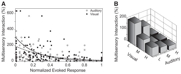
Changes in the multisensory interactive profile of AES neurons as a function of spatial location adhere to the principle of inverse effectiveness. A: a scatterplot of the magnitude of the multisensory interaction as a function of the normalized visual (black diamonds) or auditory (open circles) responses. The curves of best fit (modeled for both conditions with the exponential function [a × exp(bx)] for the visual (black dashed line, r² = 0.1238) and auditory (solid black line, r² = 0.2732) responses both show that as the magnitude of the evoked responses increase, the relative multisensory gain (i.e., interactive index) decreases. B: the bar graph divides normalized sensory evoked responses into low (L, 0–0.33), medium (M, 0.34–0.66), and high (H, 0.67–1.00) values across both sensory domains and shows that the largest multisensory interactions are found to pairings at locations where weak evoked stimulus responses are found (L visual, L auditory). In contrast, the smallest multisensory interactions are found at locations where maximal evoked stimulus responses (H visual, H auditory) are found in both domains. Note that as either of the unisensory responses increases independently there is a decrease in the size of the multisensory interaction.

SRFs represent an intermediate step in the construction of spatiotemporal receptive fields

In addition to characterizing the spatial heterogeneity of the unisensory and multisensory receptive fields of AES neurons, preliminary analyses have also focused on deconstructing these SRFs in the temporal dimension, effectively creating a spatiotemporal receptive field (STRF). Figure 7 illustrates an example of one AES neuron in which these analyses were performed. Represented are the visual, auditory, and multisensory STRFs along a single spatial plane (i.e., different points in azimuth at one elevation), along with the STRF predicted by a simple addition of the unisensory responses. Most notably, it is readily evident that the multisensory STRF differs substantially from the (V+A) prediction, and that there are changes in both the spatial and temporal domains resulting from the multisensory combination. Our goal in ongoing analyses is to better characterize the STRF architecture of AES neurons.

Fig. 7.

Temporal characteristics of stimulus-evoked responses change as a function of spatial location. Shown are spatiotemporal receptive field (STRF) plots for the visual, auditory, multisensory, and predicted addition (V+A) of the unisensory responses. Above each panel are stimulus traces that show stimulus onset and offset for each condition. The y-axis for all panels shows the azimuthal location of the stimulus (elevation was fixed at 0°). The x-axis for all panels shows the time relative to the earliest stimulus onset (t = 0). Note the difference in the temporal dynamics of the evoked responses (e.g., onset latency, duration, etc.) to the multisensory stimulus when compared with the unisensory STRFs or to the additive prediction.

DISCUSSION

In the current study, the complexity of the spatial receptive field architecture of AES neurons has been established to play an important deterministic role in the multisensory interactions seen in many of these neurons. Of greatest relevance was the fact that the spatial receptive fields of these neurons exhibited marked heterogeneity and that changes in the efficacy of the unisensory responses at different locations played a key role in dictating the multisensory interactions generated by their combination. By adhering to the principle of inverse effectiveness, in which the greatest multisensory enhancements (i.e., response gains) are seen in the combination of weakly effective stimuli, these findings make the provocative suggestion that stimulus location matters only in the way that it modulates the effectiveness of the sensory responses. Confirmation of this concept requires further study in which the efficacy of the individual sensory responses at each spatial location is systematically manipulated.

On the functional role of the AES

The cortex of the anterior ectosylvian sulcus (AES) of the cat is positioned at the apposition of the representations of three different sensory modalities. Indeed, the AES itself consists of distinct visual (AEV), auditory (FAES), and somatosensory (SIV) domains, with multisensory neurons being concentrated at the “borders” between these unisensory regions. Rather than simply being created as a by-product of the convergence of inputs from neighboring sensory representations, several observations suggest that the multisensory neurons in AES are likely to play an important functional role. First, despite the lack of any global spatiotopic organization for the visual and auditory representations in AES, individual multisensory neurons have highly overlapping receptive fields, suggesting a local organization unique to the multisensory population (Wallace et al. 2006). Second, and as established in this and previous studies (Jiang et al. 1994a; Wallace et al. 1992, 2006), multisensory AES neurons actively integrate their different sensory inputs to generate responses that differ from either of the unisensory responses and that often differ from the response predicted based on a simple addition of these responses. Such an integrated output demonstrates that these neurons are actively transforming this input information, likely in a way that facilitates the behavioral and/or perceptual role of the AES. Although this functional role has remained enigmatic, the selectivities of the neuronal populations within AES and its anatomical input/output organization point toward its playing a role in eye movements (Kimura and Tamai 1992; Tamai et al. 1989), spatial localization (Lomber and Payne 2004; Malhotra et al. 2004, 2007), motion perception (Nagy et al. 2003b; Scannell et al. 1996), and coordinate transformations between the different sensory systems (Wallace et al. 1992, 2006).

The current results bear directly on these observations and suggestions, in that they establish several important spatial processing features of AES multisensory neurons—features that provide some additional insight into the possible functional role of AES. First, they detail a striking spatial complexity to the receptive field organization of these neurons, an architecture that has been previously noted and described within the framework of panoramic localization (Benedek et al. 2004; Middlebrooks et al. 1998). In this view, AES neurons encode spatial location via unique patterns of activity to stimuli positioned at different locations within their large receptive fields. Second, and extending this concept, the current results demonstrate that receptive field heterogeneity has important consequences for the multisensory interactions seen in these neurons, specifically by modulating the relative gain seen in spatially coincident visual–auditory combinations in a way that strongly follows the principle of inverse effectiveness. Although the functional consequences of this organization await a better understanding of the perceptual role of AES, one possibility is that it acts as a spatial smoothing filter, effectively providing the AES neuron with a greater sensitivity to multisensory stimulus events throughout the extent of its large spatial receptive field. Such an organization may serve to preferentially boost the detectability of such events. A second possibility is that receptive field heterogeneity and the multisensory interactive profiles derivative of this organization play an important role in the coding and binding of multisensory motion. Indeed, receptive field heterogeneity provides an excellent substrate for the construction of unisensory motion selectivity (Clifford and Ibbotson 2002; Wagner et al. 1997; Witten et al. 2006); moreover, the gain functions described earlier might be viewed in the context of a mechanism that strives to provide a uniformity in the coding of moving visual and auditory stimuli with similar dynamics that are likely derived from the same multisensory event.

One caveat in the interpretation of the current data set is its derivation from the anesthetized preparation. Although the potential role of anesthesia in altering the response profiles of multisensory (and unisensory) neurons must be acknowledged, based on prior work examining multisensory interactions in the awake and behaving animal (Wallace et al. 1998), which showed little evidence for dramatic changes in the spatial architecture or general integrative features of multisensory neurons, we believe strongly in the utility of the anesthetized preparation. Perhaps most important, it is only in such a preparation that the time necessary for performing the comprehensive receptive field analyses described here can be carried out. Nonetheless, we agree that further elucidation of the functional role of AES awaits experiments in the awake and behaving animal.

Toward the multisensory spatiotemporal receptive field

The current results represent a critical step in the construction of a true spatiotemporal representation of multisensory neurons and their stimulus encoding features. Sensory-responsive neuronal populations are being increasingly characterized on the basis of their spatiotemporal or (for the auditory system whose most salient organizational feature is the mapping of sound frequency) spectrotemporal response profiles (Elhilali et al. 2007; Miller et al. 2002; for review see Fritz et al. 2007), a framework that allows a better detailing of the response heterogeneities and dynamics and that provides a more comprehensive description of the relationship between stimulus statistics and neuronal firing patterns (DeAngelis et al. 1995; deCharms and Zador 2000; Ghazanfar and Nicolelis 2001). Although these analyses are being increasingly used within the individual sensory systems, the current work provides the first view into this issue from the multisensory perspective, in which the dimensionality of the problem is expanded by the addition of a second sensory modality. Nonetheless, as is established by the current results, a better understanding of multisensory processes (and their likely mechanistic bases and functional roles) will undoubtedly result from the application of these more sophisticated analyses.

Better insight into the principles of multisensory integration and implications for modeling multisensory processes

As alluded to in the INTRODUCTION, the spatial, temporal, and inverse effectiveness principles of multisensory integration have provided an excellent predictive framework for understanding the consequences of multisensory interactions from the level of the single neuron to behavioral and perceptual processes (Calvert et al. 2004; Stein and Meredith 1993). Despite their utility, these principles represent but a first-order set of guidelines and often fail to capture the complete integrative capacity of individual multisensory neurons. Previous work has shown that part of this incompleteness is a result of intrinsic differences in the excitability (i.e., dynamic response range) of multisensory neurons (Perrault Jr et al. 2005). In the current study we extend the list of intrinsic factors to include the spatial organization of the multisensory receptive fields of these neurons, which plays an important role in shaping the multisensory response. Perhaps most important in this context is that the effects of the spatially heterogeneous structure of these receptive fields can be subsumed within the principle of inverse effectiveness. Given the growing interest in modeling multisensory processes (Anastasio et al. 2000, 2003; Avillac et al. 2005; Diederich and Colonius 2004; Rowland et al. 2007; Xing and Andersen 2000), these findings have important implications for the construction of any predictive model of multisensory interactions, in that they suggest that the term representative of space might be reduced into the effectiveness component of any model.

References

- Anastasio TJ, Patton PE. A two-stage unsupervised learning algorithm reproduces multisensory enhancement in a neural network model of the corticotectal system. J Neurosci. 2003;23:6713–6727. doi: 10.1523/JNEUROSCI.23-17-06713.2003. [DOI] [PMC free article] [PubMed] [Google Scholar]
- Anastasio TJ, Patton PE, Belkacem-Boussaid K. Using Bayes’ rule to model multisensory enhancement in the superior colliculus. Neural Comput. 2000;12:1165–1187. doi: 10.1162/089976600300015547. [DOI] [PubMed] [Google Scholar]
- Avillac M, Deneve S, Olivier E, Pouget A, Duhamel JR. Reference frames for representing visual and tactile locations in parietal cortex. Nat Neurosci. 2005;8:941–949. doi: 10.1038/nn1480. [DOI] [PubMed] [Google Scholar]
- Barraclough NE, Xiao D, Baker CI, Oram MW, Perrett DI. Integration of visual and auditory information by superior temporal sulcus neurons responsive to the sight of actions. J Cogn Neurosci. 2005;17:377–391. doi: 10.1162/0898929053279586. [DOI] [PubMed] [Google Scholar]
- Beauchamp MS, Argall BD, Bodurka J, Duyn JH, Martin A. Unraveling multisensory integration: patchy organization within human STS multisensory cortex. Nat Neurosci. 2004;7:1190–1192. doi: 10.1038/nn1333. [DOI] [PubMed] [Google Scholar]
- Benedek G, Eordegh G, Chadaide Z, Nagy A. Distributed population coding of multisensory spatial information in the associative cortex. Eur J Neurosci. 2004;20:525–529. doi: 10.1111/j.1460-9568.2004.03496.x. [DOI] [PubMed] [Google Scholar]
- Benedek G, Mucke L, Norita M, Albowitz B, Creutzfeldt OD. Anterior ectosylvian visual area (AEV) of the cat: physiological properties. Prog Brain Res. 1988;75:245–255. doi: 10.1016/s0079-6123(08)60483-5. [DOI] [PubMed] [Google Scholar]
- Brett-Green B, Fifkova E, Larue DT, Winer JA, Barth DS. A multisensory zone in rat parietotemporal cortex: intra- and extracellular physiology and thalamocortical connections. J Comp Neurol. 2003;460:223–237. doi: 10.1002/cne.10637. [DOI] [PubMed] [Google Scholar]
- Brosch M, Selezneva E, Scheich H. Nonauditory events of a behavioral procedure activate auditory cortex of highly trained monkeys. J Neurosci. 2005;25:6797–6806. doi: 10.1523/JNEUROSCI.1571-05.2005. [DOI] [PMC free article] [PubMed] [Google Scholar]
- Calvert GA, Spence C, Stein BE. The Handbook of Multisensory Processes. Cambridge, MA: The MIT Press; 2004. [Google Scholar]
- Clarey JC, Irvine DR. Auditory response properties of neurons in the anterior ectosylvian sulcus of the cat. Brain Res. 1986;386:12–19. doi: 10.1016/0006-8993(86)90136-8. [DOI] [PubMed] [Google Scholar]
- Clarey JC, Irvine DR. The anterior ectosylvian sulcal auditory field in the cat: I. An electrophysiological study of its relationship to surrounding auditory cortical fields. J Comp Neurol. 1990a;301:289–303. doi: 10.1002/cne.903010211. [DOI] [PubMed] [Google Scholar]
- Clarey JC, Irvine DR. The anterior ectosylvian sulcal auditory field in the cat: II. A horseradish peroxidase study of its thalamic and cortical connections. J Comp Neurol. 1990b;301:304–324. doi: 10.1002/cne.903010212. [DOI] [PubMed] [Google Scholar]
- Clemo HR, Stein BE. Somatosensory cortex: a “new” somatotopic representation. Brain Res. 1982;235:162–168. doi: 10.1016/0006-8993(82)90207-4. [DOI] [PubMed] [Google Scholar]
- Clemo HR, Stein BE. Organization of a fourth somatosensory area of cortex in cat. J Neurophysiol. 1983;50:910–925. doi: 10.1152/jn.1983.50.4.910. [DOI] [PubMed] [Google Scholar]
- Clemo HR, Stein BE. Topographic organization of somatosensory corticotectal influences in cat. J Neurophysiol. 1984;51:843–858. doi: 10.1152/jn.1984.51.5.843. [DOI] [PubMed] [Google Scholar]
- Clifford CWG, Ibbotson MR. Fundamental mechanisms of visual motion detection: models, cells and functions. Prog Neurobiol. 2002;68:409–437. doi: 10.1016/s0301-0082(02)00154-5. [DOI] [PubMed] [Google Scholar]
- DeAngelis GC, Ohzawa I, Freeman RD. Receptive-field dynamics in the central visual pathways. Trends Neurosci. 1995;18:451–458. doi: 10.1016/0166-2236(95)94496-r. [DOI] [PubMed] [Google Scholar]
- deCharms RC, Zador A. Neural representation and the cortical code. Annu Rev Neurosci. 2000;23:613–647. doi: 10.1146/annurev.neuro.23.1.613. [DOI] [PubMed] [Google Scholar]
- Diederich A, Colonius H. Bimodal and trimodal multisensory enhancement: effects of stimulus onset and intensity on reaction time. Percept Psychophys. 2004;66:1388–1404. doi: 10.3758/bf03195006. [DOI] [PubMed] [Google Scholar]
- Driver J, Noesselt T. Multisensory interplay reveals crossmodal influences on “sensory-specific” brain regions, neural responses, and judgments. Neuron. 2008;57:11–23. doi: 10.1016/j.neuron.2007.12.013. [DOI] [PMC free article] [PubMed] [Google Scholar]
- Duhamel JR, Colby CL, Goldberg ME. Ventral intraparietal area of the macaque: congruent visual and somatic response properties. J Neurophysiol. 1998;79:126–136. doi: 10.1152/jn.1998.79.1.126. [DOI] [PubMed] [Google Scholar]
- Elhilali M, Fritz JB, Chi TS, Shamma SA. Auditory cortical receptive fields: stable entities with plastic abilities. J Neurosci. 2007;27:10372–10382. doi: 10.1523/JNEUROSCI.1462-07.2007. [DOI] [PMC free article] [PubMed] [Google Scholar]
- Eordegh G, Nagy A, Berenyi A, Benedek G. Processing of spatial visual information along the pathway between the suprageniculate nucleus and the anterior ectosylvian cortex. Brain Res Bull. 2005;67:281–289. doi: 10.1016/j.brainresbull.2005.06.036. [DOI] [PubMed] [Google Scholar]
- Fritz JB, Elhilali M, David SV, Shamma SA. Does attention play a role in dynamic receptive field adaptation to changing acoustic salience in A1? Hear Res. 2007;229:186–203. doi: 10.1016/j.heares.2007.01.009. [DOI] [PMC free article] [PubMed] [Google Scholar]
- Furukawa S, Middlebrooks JC. Cortical representation of auditory space: information-bearing features of spike patterns. J Neurophysiol. 2002;87:1749–1762. doi: 10.1152/jn.00491.2001. [DOI] [PubMed] [Google Scholar]
- Ghazanfar AA, Maier JX, Hoffman KL, Logothetis NK. Multisensory integration of dynamic faces and voices in rhesus monkey auditory cortex. J Neurosci. 2005;25:5004–5012. doi: 10.1523/JNEUROSCI.0799-05.2005. [DOI] [PMC free article] [PubMed] [Google Scholar]
- Ghazanfar AA, Nicolelis MAL. The structure and function of dynamic cortical and thalamic receptive fields. Cereb Cortex. 2001;11:183–193. doi: 10.1093/cercor/11.3.183. [DOI] [PubMed] [Google Scholar]
- Ghazanfar AA, Schroeder CE. Is neocortex essentially multisensory? Trends Cogn Sci. 2006;10:278–285. doi: 10.1016/j.tics.2006.04.008. [DOI] [PubMed] [Google Scholar]
- Jiang H, Lepore F, Ptito M, Guillemot JP. Sensory interactions in the anterior ectosylvian cortex of cats. Exp Brain Res. 1994a;101:385–396. doi: 10.1007/BF00227332. [DOI] [PubMed] [Google Scholar]
- Jiang H, Lepore F, Ptito M, Guillemot JP. Sensory modality distribution in the anterior ectosylvian cortex (AEC) of cats. Exp Brain Res. 1994b;97:404–414. doi: 10.1007/BF00241534. [DOI] [PubMed] [Google Scholar]
- Kayser C, Petkov CI, Augath M, Logothetis NK. Integration of touch and sound in auditory cortex. Neuron. 2005;48:373–384. doi: 10.1016/j.neuron.2005.09.018. [DOI] [PubMed] [Google Scholar]
- Kim HG, Connors BW. Apical dendrites of the neocortex: correlation between sodium- and calcium-dependent spiking and pyramidal cell morphology. J Neurosci. 1993;13:5301–5311. doi: 10.1523/JNEUROSCI.13-12-05301.1993. [DOI] [PMC free article] [PubMed] [Google Scholar]
- Kimura A, Tamai Y. Sensory response of cortical neurons in the anterior ectosylvian sulcus, including the area evoking eye movement. Brain Res. 1992;575:181–186. doi: 10.1016/0006-8993(92)90078-n. [DOI] [PubMed] [Google Scholar]
- King AJ, Palmer AR. Integration of visual and auditory information in bimodal neurones in the guinea-pig superior colliculus. Exp Brain Res. 1985;60:492–500. doi: 10.1007/BF00236934. [DOI] [PubMed] [Google Scholar]
- Lakatos P, Chen CM, O’Connell MN, Mills A, Schroeder CE. Neuronal oscillations and multisensory interaction in primary auditory cortex. Neuron. 2007;53:279–292. doi: 10.1016/j.neuron.2006.12.011. [DOI] [PMC free article] [PubMed] [Google Scholar]
- Lomber SG, Payne BR. Cerebral areas mediating visual redirection of gaze: cooling deactivation of 15 loci in the cat. J Comp Neurol. 2004;474:190–208. doi: 10.1002/cne.20123. [DOI] [PubMed] [Google Scholar]
- Malhotra S, Lomber SG. Sound localization during homotopic and heterotopic bilateral cooling deactivation of primary and nonprimary auditory cortical areas in the cat. J Neurophysiol. 2007;97:26–43. doi: 10.1152/jn.00720.2006. [DOI] [PubMed] [Google Scholar]
- Malhotra S, Hall AJ, Lomber SG. Cortical control of sound localization in the cat: unilateral cooling deactivation of 19 cerebral areas. J Neurophysiol. 2004;92:1625–1643. doi: 10.1152/jn.01205.2003. [DOI] [PubMed] [Google Scholar]
- Mason A, Nicoll A, Stratford K. Synaptic transmission between individual pyramidal neurons of the rat visual cortex in vitro. J Neurosci. 1991;11:72–84. doi: 10.1523/JNEUROSCI.11-01-00072.1991. [DOI] [PMC free article] [PubMed] [Google Scholar]
- Meredith MA, Nemitz JW, Stein BE. Determinants of multisensory integration in superior colliculus neurons. I. Temporal factors. J Neurosci. 1987;7:3215–3229. doi: 10.1523/JNEUROSCI.07-10-03215.1987. [DOI] [PMC free article] [PubMed] [Google Scholar]
- Meredith MA, Stein BE. Interactions among converging sensory inputs in the superior colliculus. Science. 1983;221:389–391. doi: 10.1126/science.6867718. [DOI] [PubMed] [Google Scholar]
- Meredith MA, Stein BE. Spatial factors determine the activity of multisensory neurons in cat superior colliculus. Brain Res. 1986a;365:350–354. doi: 10.1016/0006-8993(86)91648-3. [DOI] [PubMed] [Google Scholar]
- Meredith MA, Stein BE. Visual, auditory, and somatosensory convergence on cells in superior colliculus results in multisensory integration. J Neurophysiol. 1986b;56:640–662. doi: 10.1152/jn.1986.56.3.640. [DOI] [PubMed] [Google Scholar]
- Meredith MA, Stein BE. Spatial determinants of multisensory integration in cat superior colliculus neurons. J Neurophysiol. 1996;75:1843–1857. doi: 10.1152/jn.1996.75.5.1843. [DOI] [PubMed] [Google Scholar]
- Middlebrooks JC, Knudsen EI. A neural code for auditory space in the cat’s superior colliculus. J Neurosci. 1984;4:2621–2634. doi: 10.1523/JNEUROSCI.04-10-02621.1984. [DOI] [PMC free article] [PubMed] [Google Scholar]
- Middlebrooks JC, Xu L, Eddins AC, Green DM. Codes for sound-source location in nontonotopic auditory cortex. J Neurophysiol. 1998;80:863–881. doi: 10.1152/jn.1998.80.2.863. [DOI] [PubMed] [Google Scholar]
- Miller LM, Escabi MA, Read HL, Schreiner CE. Spectrotemporal receptive fields in the lemniscal auditory thalamus and cortex. J Neurophysiol. 2002;87:516–527. doi: 10.1152/jn.00395.2001. [DOI] [PubMed] [Google Scholar]
- Mucke L, Norita M, Benedek G, Creutzfeldt O. Physiologic and anatomic investigation of a visual cortical area situated in the ventral bank of the anterior ectosylvian sulcus of the cat. Exp Brain Res. 1982;46:1–11. doi: 10.1007/BF00238092. [DOI] [PubMed] [Google Scholar]
- Nagy A, Eordegh G, Benedek G. Extents of visual, auditory and bimodal receptive fields of single neurons in the feline visual associative cortex. Acta Physiol Hung. 2003a;90:305–312. doi: 10.1556/APhysiol.90.2003.4.3. [DOI] [PubMed] [Google Scholar]
- Nagy A, Eordegh G, Benedek G. Spatial and temporal visual properties of single neurons in the feline anterior ectosylvian visual area. Exp Brain Res. 2003b;151:108–114. doi: 10.1007/s00221-003-1488-3. [DOI] [PubMed] [Google Scholar]
- Norita M, Mucke L, Benedek G, Albowitz B, Katoh Y, Creutzfeldt OD. Connections of the anterior ectosylvian visual area (AEV) Exp Brain Res. 1986;62:225–240. doi: 10.1007/BF00238842. [DOI] [PubMed] [Google Scholar]
- Perrault TJ, Jr, Vaughan JW, Stein BE, Wallace MT. Neuron-specific response characteristics predict the magnitude of multisensory integration. J Neurophysiol. 2003;90:4022–4026. doi: 10.1152/jn.00494.2003. [DOI] [PubMed] [Google Scholar]
- Perrault TJ, Jr, Vaughan JW, Stein BE, Wallace MT. Superior colliculus neurons use distinct operational modes in the integration of multisensory stimuli. J Neurophysiol. 2005;93:2575–2586. doi: 10.1152/jn.00926.2004. [DOI] [PubMed] [Google Scholar]
- Populin LC. Anesthetics change the excitation/inhibition balance that governs sensory processing in the cat superior colliculus. J Neurosci. 2005;25:5903–5914. doi: 10.1523/JNEUROSCI.1147-05.2005. [DOI] [PMC free article] [PubMed] [Google Scholar]
- Populin LC, Yin TC. Bimodal interactions in the superior colliculus of the behaving cat. J Neurosci. 2002;22:2826–2834. doi: 10.1523/JNEUROSCI.22-07-02826.2002. [DOI] [PMC free article] [PubMed] [Google Scholar]
- Romanski LM. Representation and integration of auditory and visual stimuli in the primate ventral lateral prefrontal cortex. Cereb Cortex. 2007;17(Suppl 1):i61–i69. doi: 10.1093/cercor/bhm099. [DOI] [PMC free article] [PubMed] [Google Scholar]
- Rowland B, Stanford T, Stein B. A Bayesian model unifies multisensory spatial localization with the physiological properties of the superior colliculus. Exp Brain Res. 2007;180:153–161. doi: 10.1007/s00221-006-0847-2. [DOI] [PubMed] [Google Scholar]
- Sato T, Schall JD. Pre-excitatory pause in frontal eye field responses. Exp Brain Res. 2001;139:53–58. doi: 10.1007/s002210100750. [DOI] [PubMed] [Google Scholar]
- Sayer RJ, Friedlander MJ, Redman SJ. The time course and amplitude of EPSPs evoked at synapses between pairs of CA3/CA1 neurons in the hippocampal slice. J Neurosci. 1990;10:826–836. doi: 10.1523/JNEUROSCI.10-03-00826.1990. [DOI] [PMC free article] [PubMed] [Google Scholar]
- Scannell JW, Sengpiel F, Tovee MJ, Benson PJ, Blakemore C, Young MP. Visual motion processing in the anterior ectosylvian sulcus of the cat. J Neurophysiol. 1996;76:895–907. doi: 10.1152/jn.1996.76.2.895. [DOI] [PubMed] [Google Scholar]
- Schlack A, Sterbing-D’Angelo SJ, Hartung K, Hoffmann KP, Bremmer F. Multisensory space representations in the macaque ventral intraparietal area. J Neurosci. 2005;25:4616–4625. doi: 10.1523/JNEUROSCI.0455-05.2005. [DOI] [PMC free article] [PubMed] [Google Scholar]
- Schroeder CE, Foxe JJ. The timing and laminar profile of converging inputs to multisensory areas of the macaque neocortex. Brain Res Cogn Brain Res. 2002;14:187–198. doi: 10.1016/s0926-6410(02)00073-3. [DOI] [PubMed] [Google Scholar]
- Schroeder CE, Lindsley RW, Specht C, Marcovici A, Smiley JF, Javitt DC. Somatosensory input to auditory association cortex in the macaque monkey. J Neurophysiol. 2001;85:1322–1327. doi: 10.1152/jn.2001.85.3.1322. [DOI] [PubMed] [Google Scholar]
- Stanford TR, Quessy S, Stein BE. Evaluating the operations underlying multisensory integration in the cat superior colliculus. J Neurosci. 2005;25:6499–6508. doi: 10.1523/JNEUROSCI.5095-04.2005. [DOI] [PMC free article] [PubMed] [Google Scholar]
- Stanford TR, Stein BE. Superadditivity in multisensory integration: putting the computation in context. Neuroreport. 2007;18:787–792. doi: 10.1097/WNR.0b013e3280c1e315. [DOI] [PubMed] [Google Scholar]
- Stein BE, Meredith MA. The Merging of the Senses. Cambridge, MA: The MIT Press; 1993. [Google Scholar]
- Stein BE, Wallace MT. Comparisons of cross-modality integration in midbrain and cortex. Prog Brain Res. 1996;112:289–299. doi: 10.1016/s0079-6123(08)63336-1. [DOI] [PubMed] [Google Scholar]
- Sugihara T, Diltz MD, Averbeck BB, Romanski LM. Integration of auditory and visual communication information in the primate ventrolateral prefrontal cortex. J Neurosci. 2006;26:11138–11147. doi: 10.1523/JNEUROSCI.3550-06.2006. [DOI] [PMC free article] [PubMed] [Google Scholar]
- Tamai Y, Miyashita E, Nakai M. Eye movements following cortical stimulation in the ventral bank of the anterior ectosylvian sulcus of the cat. Neurosci Res. 1989;7:159–163. doi: 10.1016/0168-0102(89)90056-4. [DOI] [PubMed] [Google Scholar]
- Wagner H, Kautz D, Poganiatz I. Principles of acoustic motion detection in animals and man. Trends Neurosci. 1997;20:583–588. doi: 10.1016/s0166-2236(97)01110-7. [DOI] [PubMed] [Google Scholar]
- Wallace MT, Carriere BN, Perrault TJ, Jr, Vaughan JW, Stein BE. The development of cortical multisensory integration. J Neurosci. 2006;26:11844–11849. doi: 10.1523/JNEUROSCI.3295-06.2006. [DOI] [PMC free article] [PubMed] [Google Scholar]
- Wallace MT, Meredith MA, Stein BE. Integration of multiple sensory modalities in cat cortex. Exp Brain Res. 1992;91:484–488. doi: 10.1007/BF00227844. [DOI] [PubMed] [Google Scholar]
- Wallace MT, Meredith MA, Stein BE. Multisensory integration in the superior colliculus of the alert cat. J Neurophysiol. 1998;80:1006–1010. doi: 10.1152/jn.1998.80.2.1006. [DOI] [PubMed] [Google Scholar]
- Wallace MT, Ramachandran R, Stein BE. A revised view of sensory cortical parcellation. Proc Natl Acad Sci USA. 2004;101:2167–2172. doi: 10.1073/pnas.0305697101. [DOI] [PMC free article] [PubMed] [Google Scholar]
- Wallace MT, Stein BE. Cross-modal synthesis in the midbrain depends on input from cortex. J Neurophysiol. 1994;71:429–432. doi: 10.1152/jn.1994.71.1.429. [DOI] [PubMed] [Google Scholar]
- Wallace MT, Stein BE. Development of multisensory neurons and multisensory integration in cat superior colliculus. J Neurosci. 1997;17:2429–2444. doi: 10.1523/JNEUROSCI.17-07-02429.1997. [DOI] [PMC free article] [PubMed] [Google Scholar]
- Witten IB, Bergan JF, Knudsen EI. Dynamic shifts in the owl’s auditory space map predict moving sound location. Nat Neurosci. 2006;9:1439–1445. doi: 10.1038/nn1781. [DOI] [PubMed] [Google Scholar]
- Xing J, Andersen RA. Models of the posterior parietal cortex which perform multimodal integration and represent space in several coordinate frames. J Cogn Neurosci. 2000;12:601–614. doi: 10.1162/089892900562363. [DOI] [PubMed] [Google Scholar]
- Xu L, Furukawa S, Middlebrooks JC. Auditory cortical responses in the cat to sounds that produce spatial illusions. Nature. 1999;399:688–691. doi: 10.1038/21424. [DOI] [PubMed] [Google Scholar]