Spontaneous and Task-Evoked Brain Activity Negatively Interact

Abstract

A widely held assumption is that spontaneous and task-evoked brain activity sum linearly, such that the recorded brain response in each single trial is the algebraic sum of the constantly changing ongoing activity and the stereotypical evoked activity. Using functional magnetic resonance imaging signals acquired from normal humans, we show that this assumption is invalid. Across widespread cortices, evoked activity interacts negatively with ongoing activity, such that higher prestimulus baseline results in less activation or more deactivation. As a consequence of this negative interaction, trial-to-trial variability of cortical activity decreases following stimulus onset. We further show that variability reduction follows overlapping but distinct spatial pattern from that of task-activation/deactivation and it contains behaviorally relevant information. These results favor an alternative perspective to the traditional dichotomous framework of ongoing and evoked activity. That is, to view the brain as a nonlinear dynamical system whose trajectory is tighter when performing a task. Further, incoming sensory stimuli modulate the brain's activity in a manner that depends on its initial state. We propose that across-trial variability may provide a new approach to brain mapping in the context of cognitive experiments.

Introduction

A recent revolution in neuroscience has brought the recognition that spontaneous brain activity is not only relevant but indeed crucial to normal brain functioning (Arieli et al., 1996; Yuste, 1997; Tsodyks et al., 1999; Kenet et al., 2003; Fiser et al., 2004; Raichle, 2006; Fox and Raichle, 2007; He et al., 2007; Luczak et al., 2009; Berkes et al., 2011). Despite a series of elegant studies exhibiting the influence of spontaneous brain activity on behavioral performance (Boly et al., 2007; Fox et al., 2007; Hesselmann et al., 2008a, 2008b), an important unresolved question pertains to the relationship between spontaneous brain activity and task-evoked brain responses. Currently, standard models posit that spontaneous and task-evoked brain activity linearly superimpose, such that the recorded brain activity in each single trial is the algebraic sum of the constantly changing ongoing activity and the stereotypical evoked response (Arieli et al., 1996; Azouz and Gray, 1999; Fox et al., 2006; Saka et al., 2010; Becker et al., 2011). However, interaction between ongoing and evoked brain activity was observed in anesthetized rodents under burst firing (Kisley and Gerstein, 1999), and up-and-down states (Petersen et al., 2003), such that the magnitude of the evoked activity depended on the preceding ongoing activity. Moreover, a recent study by Scheeringa et al. (2011) showed that the amplitude of evoked functional magnetic resonance imaging (fMRI) responses depended on the phase of electroencephalography (EEG) alpha oscillation at stimulus onset. Nevertheless, due to EEG's poor spatial resolution and the complex relationships between electrophysiological and fMRI signals (for reviews, see Logothetis, 2008; He and Raichle, 2009), the extent of such an interaction between ongoing and evoked brain activity in awake humans remains unclear.

The importance of this question is underscored by the fact that hitherto the most fruitful method of estimating the brain's response to a stimulus has been to average across many trials (Dawson, 1951; Gerstein, 1960; Friston et al., 1995; Dale and Buckner, 1997). The implicit assumption of this approach is that each time a stimulus is presented, the brain responds in a similar way and its response is embedded within the constantly changing ongoing activity; thus, averaging across trials suppresses the ongoing activity and recovers the evoked response. If the condition of linear superposition were fulfilled, this method would recover the evoked response veridically, so long as enough trials of the same condition are included. However, if there were variability in the evoked responses and that variability interacted with the ongoing activity, then the averaged response would provide an incomplete picture of a brain region's involvement in a task.

We set out to test the linear-superposition model. Our findings contradict this previous model and reveal instead substantial negative interaction between ongoing and evoked activity. Each time a stimulus is presented, the brain changes its state in a unique way and in a manner that depends on its initial condition. While these results do not invalidate the classical trial-averaging approach, they reveal additional behaviorally relevant information in the data not captured by these previous methods.

Materials and Methods

FMRI data acquisition.

Blood-oxygen-level-dependent (BOLD) fMRI data (4 × 4 × 4 mm³ voxels; TE, 25 ms; TR, 2.16 s) were acquired in 17 normal right-handed young adults (9 females; age, 18–27 years) using a 3T Siemens Allegra MR scanner. All subjects gave informed consent in accordance with guidelines set by the Human Studies Committee of Washington University in St. Louis. Each subject completed eight fMRI runs, each 194 frames (∼7 min) in duration. They consisted of two alternating run types. The first run type was a resting-state study in which a white crosshair was presented in the center of a black screen. Subjects were instructed to look at the crosshair, remain still, and to stay awake. The second run type was a task study in which the identical crosshair was presented, but now it occasionally changed from white to dark gray for a period of 250 ms and at times unpredictable to the subjects. The subjects were instructed to press a button with their right index finger as quickly as possible when they saw the crosshair dim. Each of these button-press runs contained 20 crosshair dims time-locked to the scanner TR, with an intertrial interval of 17.3–30.2 s. Subjects practiced this button-press task once in the scanner and before the onset of the functional scans. Anatomical MRI included a high-resolution (1 × 1 × 1.25 mm³) sagittal, T1-weighted MP-RAGE (TR, 2.1 s; TE, 3.93 ms; flip angle, 7°) and a T2-weighted fast spin-echo scan. All analyses were carried out using custom-written codes in C++ and Matlab. Other analyses using this dataset not relevant to the current hypotheses were previously published in Fox et al. (2007) and He (2011).

FMRI data preprocessing.

FMRI preprocessing steps included (1) compensation of systematic, slice-dependent time shifts; (2) elimination of systematic odd–even slice intensity difference due to interleaved acquisition; (3) rigid body correction for interframe head motion within and across runs; and (4) intensity scaling to yield a whole-brain mode value of 1000 (with a single scaling factor for all voxels). Atlas registration was achieved by computing affine transforms connecting the fMRI run first frame (averaged over all runs after cross-run realignment) with the T2-weighted and T1-weighted structural images (Ojemann et al., 1997). Our atlas-representative template included MP-RAGE data from 12 normal individuals and was made to conform to the 1988 Talairach atlas (Talairach and Tournoux, 1988). Data were resampled to 3 × 3 × 3 mm³ voxels after atlas registration. The first four frames of each fMRI run were discarded in all further analyses. The fMRI time courses from each run were detrended, and the effect of head motion and its temporal derivative were removed by linear regression. Last, the time courses were normalized by the mean of each run and transformed into percent change unit.

Definition of regions of interests.

Methods for defining the regions of interests (ROIs) have been described in detail in a previous paper (He, 2011). Thirty-one ROIs were obtained from our previous task-related functional neuroimaging studies or generated using coordinates from previous published fMRI studies. The anatomical locations, Talairach coordinates, references, and associated networks of these ROIs are listed in Table 1 of He (2011). In addition, as in He (2011), the left hand-motor cortex (LMC) was defined for each subject using task-activation patterns from the button-press fMRI runs, and the right hand-motor cortex (RMC) was defined for each subject using functional connectivity applied to resting-state fMRI runs and the individual subject's LMC region as the seed ROI. This resulted in 33 ROIs in total.

Trial-to-trial variability and task-activation analyses.

For task data, fMRI signals were epoched at eight time points surrounding stimulus onset: −1.08, 1.08, 3.24, 5.4, 7.56, 9.72, 11.88, and 14.04 s. Because it takes 2.16 s (TR, 2.16 s) to acquire one full fMRI volume (e.g., the first frame takes from 2.16 to 0 s before stimulus onset to acquire), we assigned the time of each frame to the center time of acquiring this frame. For Figure 3A, fMRI time courses were simply averaged across trials for each subject, and then averaged across subjects. For Figure 3B, SD across all trials was computed at each time point surrounding the stimulus onset in each subject. The SD time course from each subject was normalized to the first frame before stimulus onset according to the following equation:

and then averaged across subjects.

Figure 3.

A, B, Trial-averaged fMRI signal (A) and across-trial SD (B) time courses for the 33 ROIs. Each line represents one ROI (averaged across subjects). Thick black lines show the average across ROIs.

Whole-brain voxelwise analysis.

For Figures 1B and 4, activation Z-score was assessed using a random-effects analysis across subjects on fMRI signal amplitude for peak frame at 5.4 s against the prestimulus frame at −1.08 s. Trial-to-trial SD (without normalization) was compared between peak frame (5.4 s after stimulus onset) and the prestimulus frame (−1.08 s) by a t test across subjects. Both SD t score and activation Z-score were computed for all voxels within a gray-matter mask defined on the atlas image. Both the activation Z-score and the SD t score patterns were thresholded at a p < 0.05 level that was corrected for multiple comparisons using the false-discovery rate method (Benjamini and Hochberg, 1995). Plotting of slice images was done in Functional Image Viewer (http://nrg.wustl.edu/software/fiv/). Plotting of ROIs and activation Z-score on the cortical surface (Fig. 1) was produced in Caret (http://brainvis.wustl.edu/wiki/index.php/Caret:About).

Figure 1.

ROIs and task-activation/deactivation pattern. A, Thirty-one ROIs are color-coded by the networks they belong to. Non-neocortical regions included the left and right hippocampi, left and right thalami, and the right cerebellum. B, Task-activation and task-deactivation patterns obtained from whole-brain voxelwise analysis. Random-effects analysis across subjects (for peak frame at 5.4 s against the prestimulus frame) was used to obtain the Z-score.

Figure 4.

Whole-brain voxelwise analysis. A, Correlation SD change t score (t test across subjects) and task-activation Z-score (absolute value, random-effects analysis across subjects) across all voxels in the gray matter [defined by a gray-matter mask created from the atlas image; number of voxels (N), 42,001]. Both measures were assessed for peak frame at 5.4 s versus the prestimulus frame. Each dot represents one voxel. Red line indicates best linear-regression fit. B, Spatial patterns of voxels showing significant task activation/deactivation (orange and light blue respectively), significant SD decrease (red), and the overlap between them respectively (white and deep blue).

Analysis on the interaction between ongoing and evoked activity.

To assess the interaction between ongoing and evoked activity, we first defined the following parameters: (1) B equals fMRI signal amplitude at the first frame (−1.08 s before stimulus onset); (2) P equals fMRI signal amplitude at the peak frame (5.4 s after stimulus onset); and (3) D = P − B.

We then calculated r_B,D as the Pearson correlation coefficient between B and D across all trials for each subject. We averaged r_B,D across subjects after Fisher's z transformation:

where N is the number of subjects. We then obtained the averaged r_B,D value by inverting Fisher's z transformation:

This is the value plotted on the y-axis of Figure 5A (blue dots). Averaging z values instead of r values avoids bias because the former is normally distributed but the latter is not. In Figure 5B, z_B,D values were used for linear correlation.

Figure 5.

Interaction between ongoing and evoked activity. A, r_B,D is the correlation between B and D values across trials. σ_B and σ_D are the SDs of B and D values across trials respectively. r_B′,D′, σ_B′, and σ_D′ are calculated using surrogate trials from rest data. Each dot represents one ROI (red, rest data; blue, task data). B, Correlation between SD change t score (paired t test on SD between peak frame at 5.4 s and the prestimulus frame) and the difference between r_B,D and r_B′,D′ (both Fisher z transformed) across ROIs. Red line indicates the best linear-regression fit.

Next, we obtained σ_B and σ_D as the SD of B and D values across all trials in each subject, and then averaged them across subjects respectively. These were used to calculate the x-axis values in Figure 5A. For rest data, σ_B′, σ_D′, and r_B′,D′ were calculated as above, except on surrogate trials obtained by applying event triggers from the task study to the resting-state data.

Visualization of cortical activity before and after stimulus onset.

To visualize brain activity before and after stimulus onset, we plotted for each trial a stretch of prestimulus and a stretch of poststimulus activity respectively as a dot in a three-dimensional space. The three dimensions are defined as three consecutive time points before stimulus onset (−5.4, −3.24, and −1.08 s) for prestimulus activity, and around peak response for poststimulus activity (5.4, 7.56, and 9.72 s). For a cloud of dots, we can estimate the volume of the space occupied by them as the product of the confidence interval in each dimension (multiplied by a fixed parameter, which gets cancelled out in the equation below). For each ROI and each subject, we calculated a shrinking index (SI) defined as follows: Let V_post be the volume of space taken up by poststimulus data, and V_pre be the volume taken up by prestimulus data. Then:

Correlation with behavior.

To assess whether variability reduction contained behaviorally relevant information, hit trials from each subject were separated into two groups according to reaction times by a median split. A two-sample F test on variance was conducted between fast and slow trials (data were pooled across subjects) at four time points around the peak response: 3.24, 5.4, 7.56, and 9.72 s following stimulus onset respectively. Binomial statistics were used to assess significance at the population level for each time point. For visualization in Figure 7, across-trial SD for each group of task trials was normalized to the prestimulus frame, and then averaged across subjects.

Figure 7.

A, B, Trial-averaged fMRI signal (A) and across-trial SD (B) time courses for fast (solid lines) and slow (dashed lines) trials in the right cerebellum (left column) and the left hippocampus (right column). Results were averaged across subjects; error bars indicate SEM. p values are from a paired t test across subjects on across-trial SD between fast and slow trials.

Hemodynamic response modeling.

To test whether the nonlinearities present in the hemodynamic response might account for the present results, we constructed a computational model. The balloon model as detailed in Buxton et al. (1998) was adopted, with model parameters taken from the empirically fit values in Friston et al. (2000): transit time (τ₀), 0.98 s; resting oxygen extraction fraction (E₀), 0.34; stiffness (α), 0.33. The model was updated every 10 ms (sampling rate, 100 Hz) and was run for 1676.2 s (i.e., the length of our task or rest study, 4 fMRI runs, 194 frames each). We aimed to model ongoing fMRI signals with temporal properties similar to those observed empirically (He, 2011). To this end, the input to the model, cerebral blood flow (CBF, inflow), was modeled as a fractional Gaussian noise (Mandelbrot and Van Ness, 1968; Beran, 1994) with mean equaling 1, and Hurst exponent (H) equaling 0.75. The latter value was empirically determined as there was a monotonic relationship between H of the model input (CBF, inflow) and H of the model output (BOLD signal); we found that H = 0.75 for the input gave a realistic H for the simulated ongoing fMRI signal [H = 0.83, compared with H = 0.84 for empirical resting-state fMRI signals (He, 2011)]. One hundred simulations of ongoing fMRI signals were run. Detrended fluctuation analysis (for details, see He, 2011) was used to determine the Hurst exponent for the output from each simulation. The fluctuation magnitude of the simulated ongoing fMRI signal was characterized by range and SD, and was also controlled to be similar to empirical data (see Fig. 8A).

Figure 8.

Hemodynamic response modeling. A, An example of simulated ongoing fMRI signal (left) and its detrended fluctuation analysis (DFA) result (middle). Right, the fluctuation magnitude, as assessed by range and SD, as well as the DFA exponent α (which estimates directly the Hurst exponent H) are compared between simulated data and real data from resting-state study. B, Input to the balloon model for the evoked component, following Friston et al. (2000). rCBF, regional CBF. C, Simulated evoked BOLD response from the balloon model, with only the evoked CBF response as input. Ten different response amplitudes were simulated. D, Trial-averaged BOLD signals from the full balloon model, with the input including both ongoing CBF activity and evoked CBF responses. E, Correlation between the peak amplitudes of evoked BOLD response simulated in isolation (abscissa value, from C) and the trial-averaged response from the full model (ordinate value, from D). Red line indicates the unity line. F, Trial-to-trial variability (SD) time courses. As for real data, SD time courses were normalized to its value at stimulus onset. Traces in different colors show results from 10 different input amplitude values. G, Relationship between the peak amplitude of the trial-averaged responses (abscissa) and trial-to-trial variability at the same time point (ordinate) across 10 input amplitude values (r = −0.2; p = 0.58). H, Correlation between the peak amplitude of the trial-averaged responses (abscissa) and trial-to-trial variability (ordinate) at the same time point (5.4 s following stimulus onset) across 33 ROIs.

For the evoked component, we followed Friston et al. (2000) with the following model parameters: neuronal efficacy (ε), 0.5; signal decay (τ_s), 1 s, and autoregulation (τ_f), 2.46 s. We further simulated the underlying neural activity as a square wave with duration d = 0.2 s. The simulated evoked CBF response was subtracted by 1 (such that the initial value equals 0) and then added to the ongoing CBF at every time point indicated by the task trigger. This composite CBF inflow signal including both ongoing and evoked components was used as the input to the balloon model to generate the simulated BOLD signal, which was then subjected to analyses similar to those on real data for trial-averaged response and trial-to-trial variability. To cover the full range of the amplitudes of empirically observed trial-averaged responses (see Fig. 3A), we used 10 evenly spaced scaling factors for the evoked CBF response, which yielded amplitudes of trial-averaged BOLD responses from the model output in the range of 0.055 ∼ 0.55%. For each of the 10 input amplitude values, 1000 simulations were run, and the mean of 1000 simulations was reported.

Results

Seventeen healthy volunteers performed a target detection task while fMRI signals were acquired. Subjects were asked to press a button with their right index finger as quickly as possible when they detected a visual cue. Each subject performed 80 trials in total. Their hit rate on average was 98.2%. We defined a set of 31 ROIs, covering five major brain networks likely involved in this task (visual, motor, attention, saliency, and default-mode networks), as well as the thalamus, cerebellum, and hippocampus (Fig. 1A). Task-activation/deactivation patterns obtained from classical trial-averaging approach applied to the whole brain in a voxelwise manner are shown in Figure 1B. We further defined the LMC and RMC on a subject-by-subject basis (see Materials and Methods). All ROIs were selected by predefined criteria and not influenced by the current analyses.

The linear-superposition model posits that task-evoked responses do not interact with ongoing activity; hence, averaging across trials suppresses the variability in ongoing activity and recovers the “true” task-evoked response (Fig. 2i). However, at least two other scenarios are possible: task-evoked activity could interact positively (Fig. 2ii) or negatively (Fig. 2iii) with ongoing activity. In the case of a positive interaction, there is more activation or less deactivation at higher prestimulus baseline values. Contrarily, under negative interaction, there is less activation or more deactivation at higher baseline values. In both positive-interaction and negative-interaction schemes, if the sign of the evoked response flips between different baseline values (i.e., activation in some trials and deactivation in others), then single-trial brain responses would be partially cancelled out when averaged together (Fig. 2ii,iii; note that sign-flipping is a sufficient but not necessary condition for interaction).

Figure 2.

Schematics illustrating three different models about the relationship between ongoing and evoked activity: i, No interaction (also called “linear superposition”). ii, Positive interaction. iii, Negative interaction. The ongoing activity is shown in gray. Evoked responses in single trials are shown in black. Recorded brain signal in an experiment is the sum of these two. The right side of the graph shows the results of averaging across trials. For ii and iii, only one potential scenario is depicted. For example, all of single-trial responses could be activation, but the magnitude of which still positively or negatively correlates with ongoing activity. Note that the complete cancellation as depicted here is an ideal situation.

Trial-to-trial variability decreases following stimulus onset

To adjudicate between these three models, we tested their differential predictions on across-trial variability. Mathematically, the law of variance sum dictates:

where X and Y are two variables of interest, σ_X² and σ_Y² are their respective variance, and r_X,Y is the Pearson correlation coefficient between them. If r_X,Y = 0, Equation 1 reduces to Equation 2 as follows:

which says that the variances of two independent variables sum linearly.

Now, let X be the ongoing brain activity and Y be the evoked brain response due to a stimulus, then X + Y is the observed brain activity following a stimulus. We can make the following predictions:

1. Under the linear-superposition model, ongoing and evoked activity sum linearly without interaction (r_X,Y = 0) and Equation 2 holds. Since there is likely some variability in the evoked response contributing to variability in behavioral output, which justifies the routine practice of averaging brain responses according to behavioral response types (e.g., hits vs misses), we have σ_Y² > 0 and σ_X+Y² > σ_X² (i.e., cortical variability should increase after stimulus onset). Under the limit condition of a stereotypical evoked response with zero variability (σ_Y² = 0), across-trial variability stays the same after stimulus onset (σ_X+Y² = σ_X²).

2. Under the positive-interaction scheme, r_X,Y > 0; hence, variability increases after stimulus onset (σ_X+Y² > σ_X²).

3. Under the negative-interaction scheme, there are two possibilities: if $r_{X,Y}<-\frac{{\sigma }_Y}{2{\sigma }_X}<0$, then variability decreases following stimulus onset (σ_X+Y² < σ_X²); on the other hand, if $-\frac{{\sigma }_Y}{2{\sigma }_X}<r_{X,Y}<0$, then variability still increases following stimulus onset (σ_X+Y² > σ_X²).

In summary, if variability increased following stimulus onset, all three models are equally likely; by contrast, variability decrease following stimulus onset is only possible under the negative-interaction scheme.

We thus computed trial-to-trial variability of fMRI signals for each ROI as the SD across all trials at a particular time point around the stimulus onset (Fig. 3B). Remarkably, variability decreased in all 33 ROIs following stimulus onset (mean of SD across poststimulus frames is less than that of the prestimulus frame in all ROIs; peak decrease across ROIs: mean, 7.9%; range, 2.8 ∼ 14.6%). This decrease was significant in 19 of 33 ROIs (p < 0.05, uncorrected; paired t-tests across 17 subjects, poststimulus frame with the lowest SD against the prestimulus frame). Under the null hypothesis that variability does not change after stimulus onset, <2 ROIs are expected to show a significant result at a p < 0.05 level due to the 33 multiple comparisons performed. Thus, the above result is highly significant at the population level (p < 1e-16, binomial statistics). Comparing the SD time courses (Fig. 3B) with the classical trial-averaged time courses (Fig. 3A), it can be seen that around the same time that the trial-averaged mean response reaches its peak, across-trial variability reaches its trough. As mentioned above, variability decrease as observed here is only possible if ongoing and evoked activity negatively interacted with each other (Fig. 2iii).

Trial-to-trial variability across the whole brain

To ensure that our choice of ROIs did not bias the current results, we conducted a whole-brain voxelwise analysis. Across all voxels in the gray matter, 86.8% showed decreased trial-to-trial variability following stimulus onset. In addition, there was a significant correlation between variability reduction and the absolute magnitude of the classical trial-averaged response (Fig. 4A, r = −0.25, p < 1e-256; number of voxels, N = 42,001). We used the absolute magnitude here because, as Equation 1 shows, the comparison of variability between poststimulus (σ_X+Y²) and prestimulus (σ_X²) period is blind to the sign of the evoked response (Y), but only affected by the correlation between ongoing and evoked activity (r_X,Y) and, as we shall show later, r_X,Y behaves similarly regardless of whether the region is activated or deactivated.

Next, we compared the spatial pattern of task activation/deactivation with that of variability reduction (Fig. 4B). To some extent, variability reduction followed task activation in its spatial pattern. However, there are brain areas with significant variability reduction but nonsignificant change in the averaged response, and vice versa. There were slightly more voxels reaching statistical significance for task activation than for variability reduction, likely due to the lesser sensitivity of the latter measurement with equal amount of data, since each subject provided only one data point for across-trial SD, but 80 data points for the magnitude of the response (for a relevant discussion, see Gonzalez-Castillo et al., 2012). Critically, no significant variability increase was found across the brain. Such widespread variability reduction strongly supports the negative-interaction model in Figure 2iii.

Interaction between ongoing and evoked activity

Theoretically, it is not possible to directly measure the interaction between ongoing and evoked activity (r_X,Y), because the ongoing activity continues to vary after stimulus onset, and the recorded signal is the sum of this changing ongoing activity (ΔX) and the evoked activity (Y). Nonetheless, the results presented thus far suggest that there is a negative correlation between ongoing and evoked activity: given Equation 1, if variability decreases following stimulus onset (σ_X+Y² < σ_X²) as we have observed at both ROI level and whole-brain voxelwise level, then $r_{X,Y}<-\frac{{\sigma }_Y}{2{\sigma }_X}<0$.

As a proof of principle, we obtained the following measures for each ROI in every trial: peak signal amplitude (5.4 s after stimulus onset, P), baseline signal amplitude (1.08 s before stimulus onset, B), and the difference between them (D = P − B). We can now rewrite Equation 1 as follows:

where σ_P², σ_B², and σ_D² are respectively the across-trial variances of peak amplitude, baseline amplitude, and the difference between them, and r_B,D is the correlation between B and D values across trials. It is important to note that D included both the evoked response (Y) and the changing ongoing activity (ΔX). We found that for all except one ROI, $r_{B,D}<-\frac{{\sigma }_D}{2{\sigma }_B}$ (Fig. 5A, blue dots), which is consistent with our earlier observation of σ_P < σ_B (Fig. 3B).

For comparison, we applied event triggers from task study to resting-state data to obtain surrogate trials, from which similar parameters as above were defined (D′ = P′ − B′). Because resting-state data is statistically homogeneous [fMRI signals are mean and variance stationary (He, 2011)], variability should not change after artificial triggers (i.e., σ_P′ ≈ σ_B′). Given Equation 3, we can derive Equation 4:

This is the condition for variability to stay stable after stimulus onset. We calculated $-\frac{{\sigma }_{D\prime }}{2{\sigma }_{B\prime }}$ and r_B′,D′ from rest data, and found that they are indeed distributed around the unity line (Fig. 5A, red dots; the scatter around the unity line is due to finite sampling). Moreover, the difference between r_B,D and r_B′,D′ predicted the strength of variability reduction quite well (Fig. 5B, r = 0.58, p = 0.0004).

Shrinking of cortical activity space under task

Thus far we have adopted the classical view that there is the evoked activity, and then there is the ongoing activity, which continues after stimulus onset, and that the two sum (albeit nonlinearly as we have shown above) to give rise to the recorded signal after stimulus onset. However, could it be that this distinction is artificial after all? In other words, the distinction between ongoing and evoked activity in the poststimulus period makes sense if the two summed linearly; this distinction becomes blurry if linear superposition no longer holds. An alternative perspective, in line with the dynamic-systems approach to the brain (for review, see Buonomano and Maass, 2009), is that there is only one activity: the brain's trajectory in a multidimensional space before and after a stimulus. Under this perspective, we already record the brain's trajectory; there is no need to decompose it into ongoing and evoked components (which, empirically, is an ill-posed inverse problem without making assumptions, such as linear superposition).

To illustrate this idea, we visualized cortical activity before and after stimulus onset in a three-dimensional space (see Materials and Methods). We further estimated the volume of the space taken up by prestimulus and poststimulus activity respectively, and calculated an SI as the percentage of volume reduced from prestimulus to poststimulus activity. We found that the volume of the space outlined by prestimulus activity is larger than that occupied by poststimulus activity in all 33 ROIs (mean of SI across 33 ROIs, 13.6%; range, 3.1 ∼ 32.5%). A paired t test on SI across 33 ROIs showed a significant difference between prestimulus and poststimulus activity (p < 1.7e-12). Several regions with the most dramatic shrinking of cortical activity space are shown in Figure 6A. Remarkably, for some ROIs, the distribution of poststimulus activity resides completely within that of the prestimulus activity (e.g., RMC and medial prefrontal cortex), paralleling an earlier suggestion that spontaneous activity outlines the realm of possible cortical states, with poststimulus activity visiting a subset of them (Luczak et al., 2009). Importantly, the shift in the center of mass between prestimulus and poststimulus activity distributions corresponds to the classical trial-averaged mean response, while the shrinking of volume corresponds to variability reduction and can occur with (e.g., LMC and dorsal anterior cingulate cortex) or without (e.g., RMC) a change in the mean. These results echo earlier observations that variability reduction and trial-averaged response have overlaps in their spatial patterns, but can also occur independently of each other (Fig. 4B). Confirmatorily, SI correlated significantly with the strength of variability reduction (Fig. 6B, r = −0.6, p = 0.0002).

Figure 6.

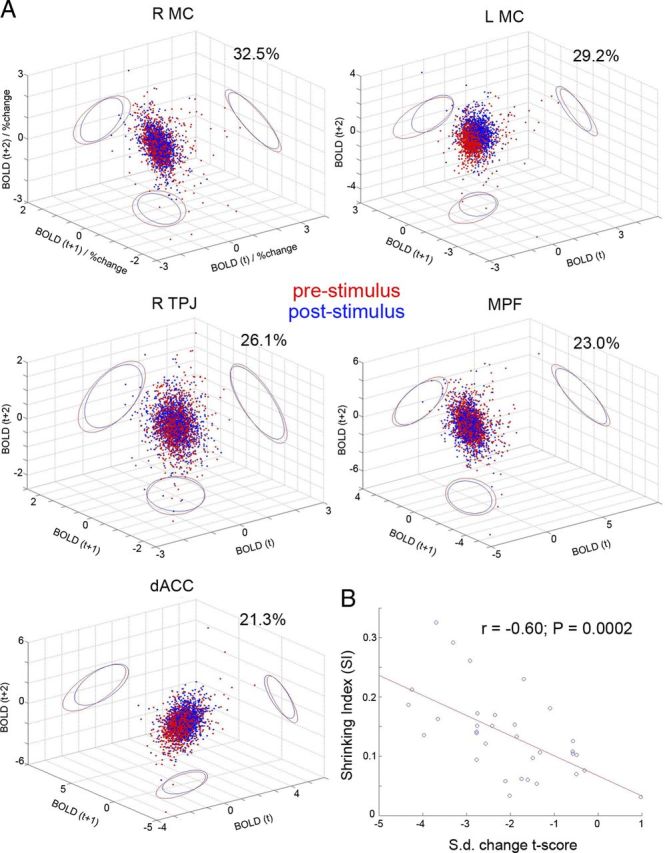
Cortical activity space analysis. A, Visualization of the prestimulus (red) and poststimulus (blue) activity across trials for selected ROIs. Data from all subjects were pooled together. Each dot represents one trial; ellipses show the 95% confidence interval of the distribution projected onto two-dimensional planes (red, prestimulus; blue, poststimulus). The SI is indicated in each graph. MC, Primary hand-motor cortex; TPJ, temporoparietal junction; MPF, medial prefrontal cortex; dACC, dorsal anterior cingulate cortex. B, Correlation between SI and the SD change t score. Each dot represents one ROI; the red line indicates the best linear-regression fit.

Trial-to-trial variability contains behaviorally relevant information

Last, we found that trial-to-trial variability carries information about behavioral outcome. The across-trial variance was compared between fast and slow trials (determined by a median split on reaction times for each subject) at four time points around the peak response. At 3.24, 5.4, 7.56, and 9.72 s following stimulus onset, there were respectively 8, 5, 5, and 6 of 33 ROIs showing a significant difference between the two groups of trials (p < 0.05, uncorrected; two-sample F test on variance). According to binomial statistics, the chance that five or more than five of 33 ROIs are individually significant at a p < 0.05 level is equal to 0.023. Thus, the above results are significant for every time point tested at the population level (8, 5, and 6 of 33 ROIs corresponds to p = 0.00017, p = 0.023, and p = 0.005 respectively).

While the above conclusion was drawn at the population level, for illustration purpose two representative ROIs are shown in Figure 7. The right cerebellum showed more variability reduction when reaction times were fast, whereas the left hippocampus showed the opposite pattern (Fig. 7B). Neither ROI differentiated between fast and slow trials in their trial-averaged time courses (Fig. 7A). We have shown earlier that a larger decrease of trial-to-trial variability reflects a stronger negative interaction between ongoing and evoked activity (Fig. 5B) and more severe tightening of the cortical activity space (Fig. 6B), suggesting that larger decrease of variability reflects more recruitment of a region in the task. Hence, these results can be interpreted as the right cerebellum being more involved in faster trials, consistent with its known functional role in motor control and timing (Ivry and Spencer, 2004). By contrast, the left hippocampus is recruited more in slower trials because the recall of personal events (e.g., planning for what to do after the scan) could distract the subject from the ongoing task and cause slower responses. This is consistent with the role of the left hippocampus in episodic memory (Squire et al., 2004).

Hemodynamic response modeling

Nonlinearities have been observed in task-evoked fMRI responses (Binder et al., 1994; Friston et al., 1998; Birn et al., 2001) and have been shown to have a hemodynamic contribution (but see Bandettini and Ungerleider, 2001; Pfeuffer et al., 2003). Thus, one question remains regarding whether the across-trial variability reduction we observed is contributed by nonlinearities in the hemodynamic response or the underlying neural activity. To address this question, we adopted a standard balloon model of neurovascular coupling (Buxton et al., 1998), whose inherent nonlinearities have been shown to successfully account for these previously reported nonlinearities in task-evoked fMRI responses (Friston et al., 2000). The balloon model assumes that the CBF response scales linearly with neural activity, while the transfer from CBF to fMRI BOLD response is highly nonlinear. Specifically, we asked the following: if evoked neural activity linearly added to ongoing neural activity, could the nonlinearity in neurovascular coupling produce the variability reduction we observed?

We first modeled ongoing fMRI signals with fluctuation magnitude (assessed by range and SD) and autocorrelation behavior (assessed by Hurst exponent; for details, see He, 2011) similar to empirically observed values from resting-state fMRI signals (Fig. 8A), and length equal to our task study. Next, at time points defined by the stimulus triggers from our task study, we added to the model input a fixed evoked CBF response (Fig. 8B). Ten evenly spaced amplitude values of the evoked CBF response were chosen to cover the entire range of the empirically observed fMRI response amplitudes (Fig. 3A), such that when simulated in isolation (i.e., without the addition of ongoing activity), the evoked fMRI response amplitudes ranged from 0.055 to 0.55% (Fig. 8C). For each input amplitude value, we recovered the trial-averaged fMRI signal from the full model with inputs including both ongoing and evoked activity (Fig. 8D), whose amplitudes were very close to the intended values (Fig. 8E). Contrary to our empirical observation (Fig. 3B), model outputs showed slightly increased trial-to-trial variability with a prolonged delay after stimulus onset at all 10 input amplitude values (Fig. 8F). The change of variability from baseline was within 2% in all cases. At the peak of the evoked response, there was no correlation between the amplitude of the averaged response and trial-to-trial variability (Fig. 8G, r = −0.2; p = 0.58), and the change of variability from baseline ranged from −0.19% to 0.65% with a predominant increase. By contrast, a similar analysis on the empirical data from 33 ROIs showed a highly significant correlation between the amplitude of the averaged response and trial-to-trial variability (Fig. 8H, r = −0.61; p < 0.0002), and the change of across-trial variability from baseline ranged from −14.6% to 3.3%, with 32 of 33 ROIs showing decreased variability.

The above results demonstrate that in the limit of no variability in the evoked response (i.e., σ_γ = 0 in Eq. 1) and no interaction between ongoing and evoked activity (i.e., r_X,Y = 0), nonlinearities in a standard balloon model of neurovascular coupling cannot reproduce variability reduction observed in our data. Anecdotally, we found that introducing variability to the evoked CBF response further increased trial-to-trial variability in the model output (i.e., simulated BOLD signal), while introducing a negative correlation between ongoing and evoked CBF activity decreased trial-to-trial variability in the model output. The full behavior of this model will be characterized in a follow-up paper.

Discussion

In summary, we report the following main findings: (1) trial-to-trial variability decreases following stimulus onset across widespread brain areas, suggesting that ongoing and evoked brain activity negatively interact with each other, such that higher prestimulus baseline results in less activation or more deactivation; (2) the space occupied by the set of potential cortical activity trajectories shrinks following stimulus onset; and (3) across-trial variability carries behaviorally relevant information. Importantly, variability reduction can occur without any significant change in the trial-averaged response (Figs. 4B, 6A); hence, it provides a novel approach to brain mapping. While we did not directly show sign flipping of single-trial responses as depicted in Figure 2ii,iii, the observation that poststimulus activity can reside completely within the realm outlined by prestimulus activity suggests that this is indeed the case in some ROIs (Fig. 6A).

Variability reduction following stimulus onset was previously reported in neuronal firing (Werner and Mountcastle, 1963; Churchland et al., 2010; Chang et al., 2012; White et al., 2012). However, given the complex relationships among the fMRI signal, neuronal firing, and local field potentials (LFPs) and the dissociation between the fMRI signal and neuronal firing under various conditions (Logothetis, 2008; Maier et al., 2008; He and Raichle, 2009), our finding of variability reduction in the fMRI signal does not follow trivially from this previous work. Importantly, the results from hemodynamic response modeling suggest that the present findings likely reflect underlying neural activity instead of a pure hemodynamic phenomenon. Nonetheless, a full understanding of the nature of neural activity underlying the present observations warrants future investigations. One potential avenue is to apply the present methods to other recording modalities, such as neuronal membrane potentials and mass neural activity reflected in electrical and magnetic fields (e.g., LFP, EEG, and magnetoencephalography). Of note, trajectory-based analyses applied to population activity recorded from the insect olfactory system have also revealed significant initial-condition-dependent stimulus modulations (Mazor and Laurent, 2005; Broome et al., 2006). Taken together with the present findings, these results suggest that the interaction between the initial state and responses to sensory inputs might be a general property of the nervous system.

Why do we find interaction between ongoing and evoked activity while earlier studies have reported linear superposition between them? Some of these previous studies computed the correlation between signal amplitudes at the prestimulus baseline and the peak response (Arieli et al., 1996; Azouz and Gray, 1999). Because the fluctuation magnitude of ongoing activity is often larger than evoked responses (Dawson, 1951; Arieli et al., 1996; Fox and Raichle, 2007), the baseline–peak correlation would be swamped by the strong autocorrelation within the ongoing activity (Arieli et al., 1996; Azouz and Gray, 1999; Bullmore et al., 2001; Sylvester et al., 2009; He, 2011). In fact, as shown in Fig 4C of Arieli et al. (1996), the autocorrelation of ongoing activity is higher than the correlation between baseline and poststimulus activity, which is consistent with the presence of a negative interaction between ongoing and evoked activity. Another previously adopted method was to use the activity in the homologous brain region as a substitute for the ongoing activity in the activated brain region [e.g., using RMC as a substitute for ongoing activity in the LMC under a right-hand motor task (Fox et al., 2006)]. However, as shown here, the homologous brain region RMC nevertheless shows significant variability reduction (Fig. 4B) and tightening of cortical activity space (Fig. 6A; in fact, the SI of RMC is the largest across 33 ROIs), indicating that it does not represent ongoing activity unaffected by the task. Last, Becker et al. (2011) presented data violating the linear-superposition model as well (Becker et al., 2011, Fig. 7), and EEG alpha-power used therein as the index of ongoing activity only accounted for 10% of trial-to-trial fMRI variance on average (see Becker et al., 2011, Fig. 9). By contrast, our results are consistent with earlier reports showing that the correlation between baseline and peak fMRI signal amplitudes depended on perceptual outcome (Hesselmann et al., 2008b; Sadaghiani et al., 2010), even though these previous studies did not directly demonstrate an interaction between ongoing and evoked activity.

The present findings have implications for studies decoding the information content of the fMRI signals using either univariate receiver–operator characteristic (ROC) curve (Sapir et al., 2005; Sylvester et al., 2009) or multivariate pattern analysis (Haxby et al., 2001; Haynes and Rees, 2006; Kriegeskorte et al., 2006; Pereira et al., 2009). These methods take advantage of both the across-trial mean response and the trial-to-trial variability. The variability reduction following stimulus onset described here would increase the decoder's ability to tell different conditions apart. It is tempting to speculate that the same mechanism might be used by the brain to more efficiently encode information and distinguish among different stimulus–behavior contingencies. Nonetheless, if the mean response is similar between conditions while the trial-to-trial variability differs, this information can be picked up by the present method but not by these decoding approaches, which rely crucially on a difference in the mean response.

Another promising recently developed method is to correlate the fMRI signal amplitude with behavioral output or model parameters on a trial-to-trial basis (Badre et al., 2012). This method also relies on a tacit assumption that there is a stereotypical evoked response under a particular value of the behavioral or model parameter, without taking into account that the evoked response could be different simply due to different baseline values. Incorporating the interaction phenomenon described here into these models (e.g., by adding the prestimulus baseline value as a separate predictor) could potentially increase the sensitivity of these methods.

It would be interesting to extend the trial-to-trial variability measure into multidimensional space. A recent study showed that the fMRI activation pattern was more reproducible under conscious perception compared with unconscious processing (Schurger et al., 2010). By using only the angle of the population vector, this study investigated the relative relationships of normalized fMRI amplitudes across space. In future studies, it would be informative to include the raw amplitude information as well, which might show a decrease of variability in both the norm and the angle of the population vector.

An important future research topic concerns the functional role(s) of variability reduction. Two possibilities, not mutually exclusive, present themselves. One is that the reduction of internal variability facilitates sensory processing (Abbott et al., 2011). Another is that variability provides an additional dimension to information coding in the brain. In parallel to our finding showing that behaviorally relevant information is sometimes encoded in the variability but not the mean of cortical responses (Fig. 7), trial-to-trial variability in membrane potentials of visual cortical cells decreases in response to high-contrast stimuli, a key mechanism that allows the system to disambiguate stimulus strength from attribute (Finn et al., 2007). Further, variability increase might carry different information from variability reduction (Briggman et al., 2005; Churchland et al., 2011). Importantly, across-trial variability might provide a useful biomarker for diagnosis of neurological/psychiatric disorders (Dinstein et al., 2012). Nonetheless, if variability were to become useful in predicting behavioral outcome on a trial-to-trial basis, single-trial correlate of the across-trial variability measure used here and elsewhere would need to be uncovered by future investigation.

Revealing the mechanism(s) of variability reduction will also be important. Of note, variability reduction to external inputs has been demonstrated in a recurrent chaotic network model (Abbott et al., 2011) and an attractor network model (Deco and Hugues, 2012); further, a mean-field model for EEG shows linear superposition and nonlinear phase resetting under different schemes of the same model (David et al., 2005). In addition, inhibitory conductance (Monier et al., 2003), neuromodulation (Goard and Dan, 2009), attention (Mitchell et al., 2007), and feedforward mechanisms (Sadagopan and Ferster, 2012) may play a role in modulating neuronal/neural-network variability as well.

Finally, the current finding that the cortical activity space shrinks following stimulus onset recalls earlier observations that the total temporal variance of signal fluctuations is reduced under task compared with rest in fMRI signals (He, 2011), neural field potentials (He et al., 2010), and neuronal membrane potentials (Poulet and Petersen, 2008). Importantly, trial-to-trial variability investigated here is not to be confused with the temporal variance of a signal, which describes the total amount of fluctuations in a behavioral state. The decrease of temporal variance during task blocks does not predict the decrease of trial-to-trial variability following stimulus onset, as the former can be homogeneous across the entire block and not time-locked to the stimulus or behavior. However, the presence of both effects in the same behavioral context (He, 2011, and the current results) point to a potential connection between them, and strengthens the impression that temporal variance decrease is due to a specific task effect. Importantly, both sets of results are consistent with an alternative view to the traditional dichotomous framework of ongoing and evoked activity. That is, to think of the brain as a dynamic system selecting its trajectory based on the context and tightening that trajectory when performing a specific task. Last but not least, in line with prior theoretical work (Buonomano and Maass, 2009), the present results suggest that incoming sensory stimuli modulate the brain's activity in a manner that depends on its initial state.

References

- Abbott LF, Rajan K, Sompolinksy H. Interactions between intrinsic and stimulus-dependent activity in recurrent neural networks. In: Ding M, Glanzman D, editors. The dynamic brain: an exploration of neuronal variability and its functional significance. New York: Oxford UP; 2011. [Google Scholar]
- Arieli A, Sterkin A, Grinvald A, Aertsen A. Dynamics of ongoing activity: explanation of the large variability in evoked cortical responses. Science. 1996;273:1868–1871. doi: 10.1126/science.273.5283.1868. [DOI] [PubMed] [Google Scholar]
- Azouz R, Gray CM. Cellular mechanisms contributing to response variability of cortical neurons in vivo. J Neurosci. 1999;19:2209–2223. doi: 10.1523/JNEUROSCI.19-06-02209.1999. [DOI] [PMC free article] [PubMed] [Google Scholar]
- Badre D, Doll BB, Long NM, Frank MJ. Rostrolateral prefrontal cortex and individual differences in uncertainty-driven exploration. Neuron. 2012;73:595–607. doi: 10.1016/j.neuron.2011.12.025. [DOI] [PMC free article] [PubMed] [Google Scholar]
- Bandettini PA, Ungerleider LG. From neuron to BOLD: new connections. Nat Neurosci. 2001;4:864–866. doi: 10.1038/nn0901-864. [DOI] [PubMed] [Google Scholar]
- Becker R, Reinacher M, Freyer F, Villringer A, Ritter P. How ongoing neuronal oscillations account for evoked fMRI variability. J Neurosci. 2011;31:11016–11027. doi: 10.1523/JNEUROSCI.0210-11.2011. [DOI] [PMC free article] [PubMed] [Google Scholar]
- Benjamini Y, Hochberg Y. Controlling the false discovery rate: a practical and powerful approach to multiple testing. J Roy Statist Soc B. 1995;57:289–300. [Google Scholar]
- Beran J. Statistics for long-memory processes. Boca Raton, FL: Chapman and Hall/CRC; 1994. [Google Scholar]
- Berkes P, Orbán G, Lengyel M, Fiser J. Spontaneous cortical activity reveals hallmarks of an optimal internal model of the environment. Science. 2011;331:83–87. doi: 10.1126/science.1195870. [DOI] [PMC free article] [PubMed] [Google Scholar]
- Binder JR, Rao SM, Hammeke TA, Frost JA, Bandettini PA, Hyde JS. Effects of stimulus rate on signal response during functional magnetic resonance imaging of auditory cortex. Brain Res Cogn Brain Res. 1994;2:31–38. doi: 10.1016/0926-6410(94)90018-3. [DOI] [PubMed] [Google Scholar]
- Birn RM, Saad ZS, Bandettini PA. Spatial heterogeneity of the nonlinear dynamics in the FMRI BOLD response. Neuroimage. 2001;14:817–826. doi: 10.1006/nimg.2001.0873. [DOI] [PubMed] [Google Scholar]
- Boly M, Balteau E, Schnakers C, Degueldre C, Moonen G, Luxen A, Phillips C, Peigneux P, Maquet P, Laureys S. Baseline brain activity fluctuations predict somatosensory perception in humans. Proc Natl Acad Sci U S A. 2007;104:12187–12192. doi: 10.1073/pnas.0611404104. [DOI] [PMC free article] [PubMed] [Google Scholar]
- Briggman KL, Abarbanel HD, Kristan WB., Jr Optical imaging of neuronal populations during decision-making. Science. 2005;307:896–901. doi: 10.1126/science.1103736. [DOI] [PubMed] [Google Scholar]
- Broome BM, Jayaraman V, Laurent G. Encoding and decoding of overlapping odor sequences. Neuron. 2006;51:467–482. doi: 10.1016/j.neuron.2006.07.018. [DOI] [PubMed] [Google Scholar]
- Bullmore E, Long C, Suckling J, Fadili J, Calvert G, Zelaya F, Carpenter TA, Brammer M. Colored noise and computational inference in neurophysiological (fMRI) time series analysis: resampling methods in time and wavelet domains. Hum Brain Mapp. 2001;12:61–78. doi: 10.1002/1097-0193(200102)12:2<61::AID-HBM1004>3.0.CO;2-W. [DOI] [PMC free article] [PubMed] [Google Scholar]
- Buonomano DV, Maass W. State-dependent computations: spatiotemporal processing in cortical networks. Nat Rev Neurosci. 2009;10:113–125. doi: 10.1038/nrn2558. [DOI] [PubMed] [Google Scholar]
- Buxton RB, Wong EC, Frank LR. Dynamics of blood flow and oxygenation changes during brain activation: the balloon model. Magn Reson Med. 1998;39:855–864. doi: 10.1002/mrm.1910390602. [DOI] [PubMed] [Google Scholar]
- Chang MH, Armstrong KM, Moore T. Dissociation of response variability from firing rate effects in frontal eye field neurons during visual stimulation, working memory, and attention. J Neurosci. 2012;32:2204–2216. doi: 10.1523/JNEUROSCI.2967-11.2012. [DOI] [PMC free article] [PubMed] [Google Scholar]
- Churchland AK, Kiani R, Chaudhuri R, Wang XJ, Pouget A, Shadlen MN. Variance as a signature of neural computations during decision making. Neuron. 2011;69:818–831. doi: 10.1016/j.neuron.2010.12.037. [DOI] [PMC free article] [PubMed] [Google Scholar]
- Churchland MM, Yu BM, Cunningham JP, Sugrue LP, Cohen MR, Corrado GS, Newsome WT, Clark AM, Hosseini P, Scott BB, Bradley DC, Smith MA, Kohn A, Movshon JA, Armstrong KM, Moore T, Chang SW, Snyder LH, Lisberger SG, Priebe NJ, et al. Stimulus onset quenches neural variability: a widespread cortical phenomenon. Nat Neurosci. 2010;13:369–378. doi: 10.1038/nn.2501. [DOI] [PMC free article] [PubMed] [Google Scholar]
- Dale AM, Buckner RL. Selective averaging of rapidly presented individual trials using fMRI. Hum Brain Mapp. 1997;5:329–340. doi: 10.1002/(SICI)1097-0193(1997)5:5<329::AID-HBM1>3.0.CO;2-5. [DOI] [PubMed] [Google Scholar]
- David O, Harrison L, Friston KJ. Modelling event-related responses in the brain. Neuroimage. 2005;25:756–770. doi: 10.1016/j.neuroimage.2004.12.030. [DOI] [PubMed] [Google Scholar]
- Dawson GD. A summation technique for detecting small signals in a large irregular background. J Physiol. 1951;115:2p–3p. [PubMed] [Google Scholar]
- Deco G, Hugues E. Neural network mechanisms underlying stimulus driven variability reduction. PLoS Comput Biol. 2012;8:e1002395. doi: 10.1371/journal.pcbi.1002395. [DOI] [PMC free article] [PubMed] [Google Scholar]
- Dinstein I, Heeger DJ, Lorenzi L, Minshew NJ, Malach R, Behrmann M. Unreliable evoked responses in autism. Neuron. 2012;75:981–991. doi: 10.1016/j.neuron.2012.07.026. [DOI] [PMC free article] [PubMed] [Google Scholar]
- Finn IM, Priebe NJ, Ferster D. The emergence of contrast-invariant orientation tuning in simple cells of cat visual cortex. Neuron. 2007;54:137–152. doi: 10.1016/j.neuron.2007.02.029. [DOI] [PMC free article] [PubMed] [Google Scholar]
- Fiser J, Chiu C, Weliky M. Small modulation of ongoing cortical dynamics by sensory input during natural vision. Nature. 2004;431:573–578. doi: 10.1038/nature02907. [DOI] [PubMed] [Google Scholar]
- Fox MD, Raichle ME. Spontaneous fluctuations in brain activity observed with functional magnetic resonance imaging. Nat Rev Neurosci. 2007;8:700–711. doi: 10.1038/nrn2201. [DOI] [PubMed] [Google Scholar]
- Fox MD, Snyder AZ, Zacks JM, Raichle ME. Coherent spontaneous activity accounts for trial-to-trial variability in human evoked brain responses. Nat Neurosci. 2006;9:23–25. doi: 10.1038/nn1616. [DOI] [PubMed] [Google Scholar]
- Fox MD, Snyder AZ, Vincent JL, Raichle ME. Intrinsic fluctuations within cortical systems account for intertrial variability in human behavior. Neuron. 2007;56:171–184. doi: 10.1016/j.neuron.2007.08.023. [DOI] [PubMed] [Google Scholar]
- Friston KJ, Holmes AP, Worsley KJ, Poline J-P, Frith CD, Frackowiak RSJ. Statistical parametric maps in functional imaging: a general linear approach. Hum Brain Mapp. 1995;2:189–210. [Google Scholar]
- Friston KJ, Josephs O, Rees G, Turner R. Nonlinear event-related responses in fMRI. Magn Reson Med. 1998;39:41–52. doi: 10.1002/mrm.1910390109. [DOI] [PubMed] [Google Scholar]
- Friston KJ, Mechelli A, Turner R, Price CJ. Nonlinear responses in fMRI: the balloon model, Volterra kernels, and other hemodynamics. Neuroimage. 2000;12:466–477. doi: 10.1006/nimg.2000.0630. [DOI] [PubMed] [Google Scholar]
- Gerstein GL. Analysis of firing pafferns in single neurons. Science. 1960;131:1811–1812. doi: 10.1126/science.131.3416.1811. [DOI] [PubMed] [Google Scholar]
- Goard M, Dan Y. Basal forebrain activation enhances cortical coding of natural scenes. Nat Neurosci. 2009;12:1444–1449. doi: 10.1038/nn.2402. [DOI] [PMC free article] [PubMed] [Google Scholar]
- Gonzalez-Castillo J, Saad ZS, Handwerker DA, Inati SJ, Brenowitz N, Bandettini PA. Whole-brain, time-locked activation with simple tasks revealed using massive averaging and model-free analysis. Proc Natl Acad Sci U S A. 2012;109:5487–5492. doi: 10.1073/pnas.1121049109. [DOI] [PMC free article] [PubMed] [Google Scholar]
- Haxby JV, Gobbini MI, Furey ML, Ishai A, Schouten JL, Pietrini P. Distributed and overlapping representations of faces and objects in ventral temporal cortex. Science. 2001;293:2425–2430. doi: 10.1126/science.1063736. [DOI] [PubMed] [Google Scholar]
- Haynes JD, Rees G. Decoding mental states from brain activity in humans. Nat Rev Neurosci. 2006;7:523–534. doi: 10.1038/nrn1931. [DOI] [PubMed] [Google Scholar]
- He BJ. Scale-free properties of the functional magnetic resonance imaging signal during rest and task. J Neurosci. 2011;31:13786–13795. doi: 10.1523/JNEUROSCI.2111-11.2011. [DOI] [PMC free article] [PubMed] [Google Scholar]
- He BJ, Raichle ME. The fMRI signal, slow cortical potential and consciousness. Trends Cogn Sci. 2009;13:302–309. doi: 10.1016/j.tics.2009.04.004. [DOI] [PMC free article] [PubMed] [Google Scholar]
- He BJ, Snyder AZ, Vincent JL, Epstein A, Shulman GL, Corbetta M. Breakdown of functional connectivity in frontoparietal networks underlies behavioral deficits in spatial neglect. Neuron. 2007;53:905–918. doi: 10.1016/j.neuron.2007.02.013. [DOI] [PubMed] [Google Scholar]
- He BJ, Zempel JM, Snyder AZ, Raichle ME. The temporal structures and functional significance of scale-free brain activity. Neuron. 2010;66:353–369. doi: 10.1016/j.neuron.2010.04.020. [DOI] [PMC free article] [PubMed] [Google Scholar]
- Hesselmann G, Kell CA, Eger E, Kleinschmidt A. Spontaneous local variations in ongoing neural activity bias perceptual decisions. Proc Natl Acad Sci U S A. 2008a;105:10984–10989. doi: 10.1073/pnas.0712043105. [DOI] [PMC free article] [PubMed] [Google Scholar]
- Hesselmann G, Kell CA, Kleinschmidt A. Ongoing activity fluctuations in hMT+ bias the perception of coherent visual motion. J Neurosci. 2008b;28:14481–14485. doi: 10.1523/JNEUROSCI.4398-08.2008. [DOI] [PMC free article] [PubMed] [Google Scholar]
- Ivry RB, Spencer RM. The neural representation of time. Curr Opin Neurobiol. 2004;14:225–232. doi: 10.1016/j.conb.2004.03.013. [DOI] [PubMed] [Google Scholar]
- Kenet T, Bibitchkov D, Tsodyks M, Grinvald A, Arieli A. Spontaneously emerging cortical representations of visual attributes. Nature. 2003;425:954–956. doi: 10.1038/nature02078. [DOI] [PubMed] [Google Scholar]
- Kisley MA, Gerstein GL. Trial-to-trial variability and state-dependent modulation of auditory-evoked responses in cortex. J Neurosci. 1999;19:10451–10460. doi: 10.1523/JNEUROSCI.19-23-10451.1999. [DOI] [PMC free article] [PubMed] [Google Scholar]
- Kriegeskorte N, Goebel R, Bandettini P. Information-based functional brain mapping. Proc Natl Acad Sci U S A. 2006;103:3863–3868. doi: 10.1073/pnas.0600244103. [DOI] [PMC free article] [PubMed] [Google Scholar]
- Logothetis NK. What we can do and what we cannot do with fMRI. Nature. 2008;453:869–878. doi: 10.1038/nature06976. [DOI] [PubMed] [Google Scholar]
- Luczak A, Barthó P, Harris KD. Spontaneous events outline the realm of possible sensory responses in neocortical populations. Neuron. 2009;62:413–425. doi: 10.1016/j.neuron.2009.03.014. [DOI] [PMC free article] [PubMed] [Google Scholar]
- Maier A, Wilke M, Aura C, Zhu C, Ye FQ, Leopold DA. Divergence of fMRI and neural signals in V1 during perceptual suppression in the awake monkey. Nat Neurosci. 2008;11:1193–1200. doi: 10.1038/nn.2173. [DOI] [PMC free article] [PubMed] [Google Scholar]
- Mandelbrot BB, Van Ness JW. Fractional Brownian motions, fractional noises and applications. SIAM Review. 1968;10:422–437. [Google Scholar]
- Mazor O, Laurent G. Transient dynamics versus fixed points in odor representations by locust antennal lobe projection neurons. Neuron. 2005;48:661–673. doi: 10.1016/j.neuron.2005.09.032. [DOI] [PubMed] [Google Scholar]
- Mitchell JF, Sundberg KA, Reynolds JH. Differential attention-dependent response modulation across cell classes in macaque visual area V4. Neuron. 2007;55:131–141. doi: 10.1016/j.neuron.2007.06.018. [DOI] [PubMed] [Google Scholar]
- Monier C, Chavane F, Baudot P, Graham LJ, Frégnac Y. Orientation and direction selectivity of synaptic inputs in visual cortical neurons: a diversity of combinations produces spike tuning. Neuron. 2003;37:663–680. doi: 10.1016/s0896-6273(03)00064-3. [DOI] [PubMed] [Google Scholar]
- Ojemann JG, Akbudak E, Snyder AZ, McKinstry RC, Raichle ME, Conturo TE. Anatomic localization and quantitative analysis of gradient refocused echo-planar fMRI susceptibility artifacts. Neuroimage. 1997;6:156–167. doi: 10.1006/nimg.1997.0289. [DOI] [PubMed] [Google Scholar]
- Pereira F, Mitchell T, Botvinick M. Machine learning classifiers and fMRI: a tutorial overview. Neuroimage. 2009;45:S199–S209. doi: 10.1016/j.neuroimage.2008.11.007. [DOI] [PMC free article] [PubMed] [Google Scholar]
- Petersen CC, Hahn TT, Mehta M, Grinvald A, Sakmann B. Interaction of sensory responses with spontaneous depolarization in layer 2/3 barrel cortex. Proc Natl Acad Sci U S A. 2003;100:13638–13643. doi: 10.1073/pnas.2235811100. [DOI] [PMC free article] [PubMed] [Google Scholar]
- Pfeuffer J, McCullough JC, Van de Moortele PF, Ugurbil K, Hu X. Spatial dependence of the nonlinear BOLD response at short stimulus duration. Neuroimage. 2003;18:990–1000. doi: 10.1016/s1053-8119(03)00035-1. [DOI] [PubMed] [Google Scholar]
- Poulet JF, Petersen CC. Internal brain state regulates membrane potential synchrony in barrel cortex of behaving mice. Nature. 2008;454:881–885. doi: 10.1038/nature07150. [DOI] [PubMed] [Google Scholar]
- Raichle ME. Neuroscience. The brain's dark energy. Science. 2006;314:1249–1250. [PubMed] [Google Scholar]
- Sadaghiani S, Hesselmann G, Friston KJ, Kleinschmidt A. The relation of ongoing brain activity, evoked neural responses, and cognition. Front Syst Neurosci. 2010;4:20. doi: 10.3389/fnsys.2010.00020. [DOI] [PMC free article] [PubMed] [Google Scholar]
- Sadagopan S, Ferster D. Feedforward origins of response variability underlying contrast invariant orientation tuning in cat visual cortex. Neuron. 2012;74:911–923. doi: 10.1016/j.neuron.2012.05.007. [DOI] [PMC free article] [PubMed] [Google Scholar]
- Saka M, Berwick J, Jones M. Linear superposition of sensory-evoked and ongoing cortical hemodynamics. Front Neuroenergetics. 2010;2 doi: 10.3389/fnene.2010.00023. [DOI] [PMC free article] [PubMed] [Google Scholar]
- Sapir A, d'Avossa G, McAvoy M, Shulman GL, Corbetta M. Brain signals for spatial attention predict performance in a motion discrimination task. Proc Natl Acad Sci U S A. 2005;102:17810–17815. doi: 10.1073/pnas.0504678102. [DOI] [PMC free article] [PubMed] [Google Scholar]
- Scheeringa R, Mazaheri A, Bojak I, Norris DG, Kleinschmidt A. Modulation of visually evoked cortical FMRI responses by phase of ongoing occipital alpha oscillations. J Neurosci. 2011;31:3813–3820. doi: 10.1523/JNEUROSCI.4697-10.2011. [DOI] [PMC free article] [PubMed] [Google Scholar]
- Schurger A, Pereira F, Treisman A, Cohen JD. Reproducibility distinguishes conscious from nonconscious neural representations. Science. 2010;327:97–99. doi: 10.1126/science.1180029. [DOI] [PubMed] [Google Scholar]
- Squire LR, Stark CE, Clark RE. The medial temporal lobe. Annu Rev Neurosci. 2004;27:279–306. doi: 10.1146/annurev.neuro.27.070203.144130. [DOI] [PubMed] [Google Scholar]
- Sylvester CM, Shulman GL, Jack AI, Corbetta M. Anticipatory and stimulus-evoked blood oxygenation level-dependent modulations related to spatial attention reflect a common additive signal. J Neurosci. 2009;29:10671–10682. doi: 10.1523/JNEUROSCI.1141-09.2009. [DOI] [PMC free article] [PubMed] [Google Scholar]
- Talairach J, Tournoux P. Co-planar stereotaxic atlas of the human brain. New York: Georg Thieme; 1988. [Google Scholar]
- Tsodyks M, Kenet T, Grinvald A, Arieli A. Linking spontaneous activity of single cortical neurons and the underlying functional architecture. Science. 1999;286:1943–1946. doi: 10.1126/science.286.5446.1943. [DOI] [PubMed] [Google Scholar]
- Werner G, Mountcastle VB. The variability of central neural activity in a sensory system, and its implications for the central reflection of sensory events. J Neurophysiol. 1963;26:958–977. doi: 10.1152/jn.1963.26.6.958. [DOI] [PubMed] [Google Scholar]
- White B, Abbott LF, Fiser J. Suppression of cortical neural variability is stimulus- and state-dependent. J Neurophysiol. 2012;108:2383–2392. doi: 10.1152/jn.00723.2011. [DOI] [PMC free article] [PubMed] [Google Scholar]
- Yuste R. Introduction: spontaneous activity in the developing central nervous system. Semin Cell Dev Biol. 1997;8:1–4. doi: 10.1006/scdb.1996.0114. [DOI] [PubMed] [Google Scholar]