

Abstract
Recurrent neural networks (RNNs) are useful tools for learning nonlinear relationships in time series data with complex temporal dependences. In this paper, we explore the ability of a simplified type of RNN, one with limited modifications to the internal weights called an echostate network (ESN), to effectively and continuously decode monkey reaches during a standard center-out reach task using a cortical brain–machine interface (BMI) in a closed loop. We demonstrate that the RNN, an ESN implementation termed a FORCE decoder (from first order reduced and controlled error learning), learns the task quickly and significantly outperforms the current state-of-the-art method, the velocity Kalman filter (VKF), using the measure of target acquire time. We also demonstrate that the FORCE decoder generalizes to a more difficult task by successfully operating the BMI in a randomized point-to-point task. The FORCE decoder is also robust as measured by the success rate over extended sessions. Finally, we show that decoded cursor dynamics are more like naturalistic hand movements than those of the VKF. Taken together, these results suggest that RNNs in general, and the FORCE decoder in particular, are powerful tools for BMI decoder applications.
Introduction
Brain–machine interfaces (BMIs) translate neural activity into control signals for prosthetic devices, such as computer cursors and robotic limbs, aiming to offer disabled patients greater interaction with the world. Despite many compelling proof-of-concept animal experiments [1–8] and human clinical trials [9, 10], a fundamental limitation of these systems is the performance of the decoder. A standard decoder in BMI systems, the VKF [5], has seen wide application and performs better than its static counterpart, the linear decoder [1, 3, 7, 11], presumably due to the Kalman filter's ability to capture aspects of the plant dynamics in the kinematic data. However, due to the linearity of the Kalman filter, the power of the VKF must be limited in contexts where the relationship between the inputs and outputs is nonlinear. While the nature of motor representation in the pre-motor dorsal cortex (PMd) and motor cortex (M1) remains an open question [12–18], it seems likely that the relationship between neural activity in these areas and arm kinematics is nonlinear. Thus, it is appropriate to explore nonlinear methods when decoding arm kinematics from PMd/M1 activity.
A standard class of models for learning nonlinear relationships is the neural network. FNNs7 are important standard tools in machine learning [19], whose computational power derives from both nonlinearity and the distributed nature of the computation [20]. However, despite some initial exploration of FNNs to BMI [3, 21, 22], it is not clear that FNNs are a beneficial tool for BMIs as they have not outperformed the linear filter substantially. This is primarily because they lack network dynamics and because their input–output relationships are difficult to understand. The latter in turn makes model selection and optimization more difficult.
The dynamical version of a neural network, the recurrent neural network (RNN), so named because of the feedback connections that create ongoing internal dynamics (network neurons' activities are a function of their own past), have been proposed for almost as long as FNNs [23, 24]. The RNN appears to have all the criteria for an excellent BMI decoder because it has network dynamics and the computation is both nonlinear and distributed. Unfortunately, due to the complexities involved in training them [25, 26], RNNs have seen more limited application and have remained firmly in the realm of academic research. It is worth noting that Fetz anticipated their potential utility for BMI over ten years ago [27], and in basic neuroscience research ten years before that [28–30].
Recently, there has been some progress on the difficult problem of training RNNs. Specifically, Jaeger and colleagues proposed the echostate network (ESN), defined as a randomly initialized RNN, where synaptic changes are limited to the output units of the network [31]. The output of the ESN is a linear readout of the recurrent, nonlinear units and may potentially feedback to the network, thus modifying the network's dynamics (see figure 1 for a sketch). Due to the explicitly constrained learning problem, ESNs are easily trained and were shown to solve practical spatiotemporal problems [31]. More recently, we proposed a new, online learning rule for ESNs, called the FORCE learning rule (first order reduced and controlled error), enabling ESNs to operate far more stably and in a more powerful regime [32].
Figure 1.
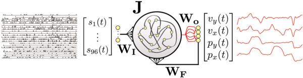
Network schematic of the FORCE decoder with inputs and outputs. The FORCE decoder is a recurrent neural network with effective internal connections defined by the matrix gJ + WFWOT, with g a global scale factor. The input to the decoder is the set of binned spikes s1(t), …, s96(t) from the multi-electrode array implanted in PMd and is multiplied by the weights in the matrix WI. The network output is a decoded, normalized version of the monkey's arm position and velocity in the x and y directions, denoted px(t), py(t), vx(t), vy(t) for the normalized position and velocity signals, respectively (red traces on the right). The decoder is trained solely by modifying the weights WO in red. The output is fed back to the network through weights WF, allowing the decoded positions and velocities to modify the network dynamics. Thus, the network dynamics are a combination of the binned spikes, the activity resulting from the internal connectivity and the decoded position and velocity signals. The actual decode during BMI was a linear combination of position and integrated velocity signals rescaled to the physical dimensions of the workspace.
There have been some applications of RNNs to the problem of BMI. Sanchez and colleagues used a RNN to decode monkey hand position of a stereotyped reaching movement from offline array recordings of posterior parietal, premotor and motor neurons [33]. Also, Gunduz and colleagues trained an ESN to decode two-dimensional hand trajectories from offline human ECoG recordings [34].
Given these recent advances in RNNs, we investigated whether we could successfully design and use a RNN as the decoder in the online BMI setting. Specifically, we studied a RNN, based on the ESN architecture and using the FORCE learning rule, applied to the online, continuous decode of monkeys' arm kinematics from a 96-channel array in M1 or M1/PMd. We demonstrate not only its successful operation but also significantly improved performance when compared to the current state-of-the-art velocity Kalman filter algorithm.
Methods
Experimental methods
We trained monkeys to acquire targets with a cursor controlled by either native arm movement or neural activity. The monkeys were trained to make point-to-point reaches in a 2D fronto-parallel plane with a virtual cursor controlled by the contralateral arm or by a neural decoder [35]. In the center-out task, monkeys had to acquire targets that alternated from the center of the workspace to one of eight preset peripheral locations located 8 cm away from the center. In the pinball task, targets would appear randomly in the workspace. In both tasks, upon successfully holding the cursor within 2 cm of the target for 500 ms, the monkeys received a liquid reward. The virtual cursor and targets were presented in a 3D environment (MSMS, MDDF, USC, Los Angeles, CA). The hand position was measured with an infrared reflective bead-tracking system at 60 Hz (Polaris, Northern Digital, Ontario, Canada). Spike counts were collected by applying a single negative threshold, set to 4.5× root mean square of the spike band of each neural channel. Behavioral control and neural decode were run on separate PCs using the xPC Target platform (Mathworks, Natick, MA) with communication latencies of 3 ms [36]. This system enabled millisecond-timing precision for all computations. Neural data were initially processed by the Cerebus recording system (Blackrock Microsystems Inc., Salt Lake City, UT) and were available to the behavioral control system within 5 ± ms. Visual presentation was provided via two LCD monitors with refresh rates at 120 Hz, yielding frame updates within 7 ± 4 ms. Two mirrors visually fused the displays into a single 3D percept for the user, creating a Wheatstone stereograph (see figure 2 in [35]).
Figure 2.
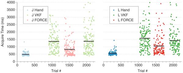
Representative ABA block trials for monkey J and monkey L. Representative days are shown for both monkeys. Shown are the target acquire times for each trial (ms). First, 200+ hand trials were collected as a baseline at the beginning of the session (acquire times shown in light blue and blue). The VKF decoder was run for 300+ trials (light green and green), followed by the FORCE decoder for 300+ trials (acquire times shown in light red and red) and finally the VKF decoder again for 300+ trials. The block average acquire times are shown as black lines across the trial blocks. Trials numbers without data points were used for either training data or for `burn' trials that allowed the monkey to habituate the new decoder.
All procedures and experiments were approved by the Stanford University Institutional Animal Care and Use Committee. Experiments were conducted with adult male rhesus macaques (L and J), implanted with 96-electrode Utah arrays (Blackrock Microsystems Inc., Salt Lake City, UT) using standard neurosurgical techniques [37–39]. Monkeys L and J were implanted 37 months and 18 months prior to the primary experiments, respectively. An electrode array was implanted at the border of the dorsal aspect of the premotor cortex (PMd) and primary motor cortex (M1) for monkey L and in M1 for monkey J, as estimated visually from anatomical landmarks.
Velocity Kalman filter
In this study, we compared the performance of the RNN to the decoder widely viewed as the state-of-the-art in the field, the `velocity Kalman filter'. The VKF linearly tracks the evolution of a kinematic state (in this case, the velocity of the cursor on the screen) over time, using discretized observations (binned neural data) to update estimates of the state. The kinematic state, xVKF (t) = [vx(t), vy(t), 1], models velocity and allows for a fixed bias. The observations of the VKF are the neural data, denoted y(t), and are used to update the state estimate.
The VKF was constructed and run in a similar fashion as in previous work [11]. Specifically, the VKF assumes a linear relationship between the kinematic state and neural observations both subject to additive Gaussian noise. The system equations are as follows:
| (2.1) |
| (2.2) |
where A is the k × k state update matrix and C is the I × k observation matrix, where k is the dimensionality of the kinematic state (3, in this case of the VKF) and I is the dimensionality of the neural observations (number of channels being recorded, 96 in this case). The vectors w(t) and q(t) are Gaussian noise sources for each system, with w(t) ~ N(0, W) and q(t) ~ N(0, Q), where W and Q are the sample noise covariance matrices of w(t) and q(t), respectively. The parameters for the Kalman filter are thus the set of four matrices {A, C, W, Q}. Each can be efficiently and analytically inferred given a training set. Using time-aligned and binned kinematic (X) and neural (Y) data (binned at the same width as the testing set, 50 ms in this case), we fit the parameters for the Kalman filter using the following matrices:
| (2.3) |
| (2.4) |
| (2.5) |
| (2.6) |
where D is the number of samples in the training set. X1 and X2 are nearly identical to X, but contain one less column of data (X1 is missing the last column and X2 is missing the first column). These parameters are used in the VKF decoder and run in real time on the decoding computer.
The actual velocities used to generate the cursor position were κ[vx(t), vy(t)], with the parameter κ defined as the output gain of the filter (typically κ = 1). However, we wanted to test whether or not simply modulating the velocities of the VKF would result in better performance, so we modulated κ between 1.0 and 2.0 in some studies. Note that equations (2.1) and (2.2) were still used to update the Kalman filter and κ was merely an output gain that we applied to the cursor output only.
Recurrent neural network
Our generic recurrent network model is defined by an N-dimensional vector of activation variables, x, and a vector of corresponding `firing rates', r = tanh(x). Both x and r are continuous in time and take continuous values. The equation governing the dynamics of the activation vector is of the standard form
| (2.7) |
The N × N matrix J describes the weights of the recurrent connections of the network, and we take it to be randomly sparse, meaning that only n < N randomly chosen elements are non-zero in each of its rows. The non-zero elements of J are drawn independently from a Gaussian distribution with zero mean and variance 1/n. The parameter gprovides a global parameter that controls the strength of the recurrent network's initial internal coupling and is a crucial parameter that is adjusted in a task-by-task basis. The input to the network, u(t), an I-dimensional vector, is fed in through the matrix of weights WI, with dimension N × I, again taken to be randomly sparse with i < I randomly chosen, non-zero elements in each row that are drawn independently from a Gaussian distribution with zero mean and variance 1/i. The parameter h is a global scaling of the input. Each neuron receives a weighted sum of the M-dimensional output of the network z(t) (defined below). The feedback weights are defined by the matrix WF, of size N × M, again taken to be randomly sparse with m < M randomly chosen8 non-zero elements in each row that are drawn independently from a Gaussian distribution with zero mean and variance 1/m. The neurons receive a constant bias b, drawn from a Gaussian distribution with standard deviation σb. The neuronal time constant τ sets the time scale of the network.
The output of the network is a weighted sum of the network firing rates, defined by the equation
| (2.8) |
where WO is an N × M matrix whose elements are initialized to zero. The only matrix (or vector) learned in this network is WO. As mentioned, the output is fed back to the network via a matrix of weights WF. Thus, network dynamics arising from internal connectivity are controlled by the effective connectivity matrix, gJ+WFWOT, and so training WO allows a rank-M modification to the matrix governing the recurrent activity in the network.
The network was trained online9 with the FORCE learning algorithm, as described in [32]. Briefly, the FORCE learning rule is a supervised learning algorithm for RNNs designed to stabilize their complex and potentially chaotic dynamics using very fast weight changes and strong feedback. The precise details of how the algorithm works are described in [32]. For practical implementations, we describe here the recursive least-squares (RLS) algorithm [40] for the network defined by equations (2.7) and (2.8).
First, we define a continuous error signal
| (2.9) |
for a given continuous target signal f(t). Using RLS, the modification to the mth column of WO is defined by
| (2.10) |
where Δtl is the time increment for the learning step, which need not be the same as the simulation time step, and P(t) is an N × N matrix representing the inverse correlation matrix. It is updated at the same time as the weights according to the rule
| (2.11) |
The algorithm also requires an initial value for P, which is taken to be
| (2.12) |
where α−1 takes on both the roles of the initial learning rate and regularizer for the learning algorithm.
We applied network equations (2.7) and (2.8) and the FORCE learning rule defined by equations (2.9) through (2.12) to our BMI task of continuous hand decode by choosing as inputs the binned neural signals and for the outputs, the monkeys' arm kinematics. A schematic is shown in figure 1. Specifically, the inputs to the network, u(t), were the 96-dimensional (I = 96) multi-unit activity of spike counts (collected as described above), binned to the simulation time step of the network, Δt. We trained the network to output a four-dimensional (M = 4) signal, z(t), representing normalized position and velocity through time in both the horizontal (x) and vertical (y) spatial dimensions. We calculated the hand velocities from the positions numerically using central differences. Finally, both position and velocity datasets were then interpolated up to 1 ms and then downsampled to the appropriate simulation Δt, which differed for the two monkeys. In order to provide the output units with a constant bias, the firing rate of the first neuron of the network, r1(t), was set to a constant of 1.
Since the FORCE decoder outputs both normalized position and velocity, we combined both for our final decode. The decode used during the BMI mode, dx(t), dy(t), was a mix of both velocity and position, defined by
| (2.13) |
| (2.14) |
where vx, vy, px, py are the normalized velocity and positions in the x and y dimensions, β = 0.95 and γv, γp are factors that convert from the normalized velocity and position, respectively, to the physical values associated with the workspace.
The parameters of the model are listed in table 1. Many of the parameters were the same across monkeys but five were chosen separately (see section 4 for an explanation of choices). These are listed at the top of table 1. A network was simulated by integrating equation (2.7) using the Euler method at a time step of Δt = τ/5 and then evaluating equation (2.8). The learning algorithm was applied every two simulation time steps (Δtl = 2Δt), with an initial diagonal loading of the inverse correlation matrix with α = 100. The input data u(t) and target output f(t) were recorded as described in the experimental methods and processed as described above. Roughly 300–500 center-out reaches were collected and used as training data with 20–50 reaches left for an offline cross validation. The network was trained on the data for four passes of the data on average, which took about 15 min. During training, each neuron had Gaussian noise with 0 mean and standard deviation 0.01 injected into it. After training, the network was placed into the embedded real-time environment (xPC), in exactly the same way as the VKF, to operate online in the BMI mode. Specifically, at each time point, the RNN module received binned spikes and output the current estimate of the hand position, which was used to display the cursor position on the screen. During the BMI mode, the network was run without any noise.
Table 1.
Network parameters for monkeys J and L. The first five parameters differ between the monkeys and reflect a trade-off between accurate kinematic dynamics (monkey J, with more active channels on the array) versus an accurate decode from an array with fewer active channels (monkey L).
| Monkey J | Monkey L | |
|---|---|---|
| Δ t | 15 ms | 25 ms |
| τ | 75 ms | 125 ms |
| N | 1200 | 1500 |
| n | 120 | 150 |
| g | 0.5 | 1.0 |
| h | 0.5 | 0.5 |
| i | 12 | 12 |
| m | 2 | 2 |
| σ b | 0.025 | 0.025 |
Δt: simulation time step, τ: the neuronal time constant of the network units, N: the number of RNN neurons, n: the number of connections from one neuron to another, g: global scaling of internal connections, h: global scaling of inputs, i: the number of inputs to each RNN neuron, m: the number of outputs fed back to each RNN neuron, σb: the standard deviation of the bias current to each RNN neuron.
Results
Both the VKF and FORCE decoders were trained to generate monkey arm kinematics data from multi-unit arrays implanted in PMd/M1 in a center-out 8 reach task. In this task, a monkey is instructed to move a virtual cursor to instructed targets located along the periphery and the center of a circle. The subject must hold the target for 500 ms to successfully complete the trial. To assess the VKF and FORCE decoders, we used a basic trial block structure (a representative day for each monkey is shown in figure 2). First, the monkey performed a set of 200 baseline hand measurements. The target acquire times are shown in light blue and blue for monkeys J and L, respectively. The target acquire time is the time it took, after target onset, for the monkey to move the cursor into the target acceptance window and hold it there for 500 ms. After performing another 500 native hand measurements (not shown), used for training, the monkey then transitioned to the VKF decoder for a block of 300 trials (acquire times shown in light green and green for monkey J and monkey L), then the FORCE decoder for 300 trials (light red and red for monkey J and monkey L), and finally the VKF decoder for another 300 trials. In order to allow the monkey to habituate to a new decoder, we allowed the monkey about 100 initial `burn' trials that were not used in the performance statistics. In this way, we tested each monkey in an ABA block structure. For monkey J, we measured four days of ABABA blocks. For monkey L, we measured two days of ABA blocks and two days of AB blocks, since monkey L sometimes stopped working in the last block of VKF trials, though never during the block of FORCE trials. A video demonstrating the quality of the FORCE decoder can be found in the online supplemental materials available at stacks.iop.org/JNE/9/026027/mmedia.
Because the FORCE decoder showed significantly faster mean speed than the VKF decoder (speeds are reported later), we experimented with the output gain of the VKF decoder, κ in equation (2.2), to check whether simply increasing the output gain might increase the speed and performance of the decoder. While the speed of the cursor was increased by increasing the output gain of the Kalman filter (supplemental figure 1 available at stacks.iop.org/JNE/9/026027/mmedia), the performance of the online decoder was decreased in rough proportion to the increase of the output gain above 1 (supplemental figure 2 available at stacks.iop.org/JNE/9/026027/mmedia). This is because uniformly increasing the velocity of the cursor makes it more difficult to satisfy the constraint of a 500 ms hold time within the target window. This hold time is required to count a successful trial and is a critical test of cursor controllability. Therefore, despite the difference in mean cursor speeds of the VKF and FORCE decoders, we report the comparisons of the VKF decoder performance with unity output gain (κ = 1), which gave the best performance for both monkeys, against the performance of the FORCE decoder.
We tested the performance of the decoders in BMI mode in a number of ways, including computing three summary statistics, the success rate, the distance ratio and the average error angle (summarized in table 2). The success rates across all trials for monkey J for hand, VKF decoder and FORCE decoder were 99.9%, 97.5% and 99.5%, respectively. The success rates of monkey L were 100%, 95.3% and 92.8%, respectively. We also measured the distance ratio metric [41], which gives a measure of cursor trajectory quality that is independent of cursor speed. The distance ratio is a unitless quantity and is defined as the actual distance traveled from the time of target onset to target acquisition, divided by the straight line distance from the start location to the target. A smaller distance ratio is better. The distance ratios were 1.16 ± 0.56, 2.30 ± 1.41 and 1.94 ± 1.17 for the hand, VKF decoder and FORCE decoder across all trials for monkey J (mean and standard deviation). The distance ratios were 1.08 ± 0.21, 2.74±1.36 and 1.68±0.91, respectively, for monkey L across all trials. We also report the average error angle, which is the angle between the instantaneous velocity vector and the vector pointing from the cursor center to the target center, averaged across each time step of the trajectory from target onset to final target acquisition. The average error angles across all targets in degrees for monkey J (mean and standard deviation) were 55.2 ± 19.2°, 73.2 ± 18.3° and 63.2 ± 16.6° for hand, VKF decoder and FORCE decoder, respectively. For monkey L, they were 50.5 ± 18.0°, 65.6 ± 13.7° and 55.7 ± 18.2°, respectively.
Table 2.
Summary performance statistics for monkeys J and L for native hand, the VKF decoder and the FORCE decoder.
| Monkey J | Monkey L | |||||
|---|---|---|---|---|---|---|
| Hand | VKF | FORCE | Hand | VKF | FORCE | |
| Success rate | 99.9% | 97.5% | 99.5% | 100% | 95.3% | 92.8% |
| Distance ratio | 1.16 ± 0.56 | 2.30 ± 1.41 | 1.94 ± 1.17 | 1.08 ± 0.21 | 2.74 ± 1.36 | 1.68 ± 0.91 |
| Average error angle | 55.2 ± 19.2° | 73.2 ± 18.3° | 63.2 ± 16.6° | 50.5 ± 18.0° | 65.6 ± 13.7° | 55.7 ± 18.2° |
Success rate: the percentage of correct trials divided by the total number of trials. To be considered a successful trial, we enforced a 500 ms hold time of the cursor on the target. Distance ratio: a unitless measure of cursor trajectory quality that is independent of cursor speed. A smaller distance ratio is better. Average error angle: the angle between the instantaneous velocity vector and the vector pointing from the cursor center to the target center, averaged across each time step of the trajectory from target onset to final target acquisition.
In order to understand the different performance of the two decoders, we also studied the mean distance to the target as a function of time for both decoders and both monkeys (figure 3). Specifically, these plots show the average distance of the cursor to the target at each time point, averaged across trials. The thicker line shows the average `dial-in' time. Its borders are defined by the first and last times the monkey's cursor went into the target acceptance window, on average. The length of this thick line measures how well the monkey can stop the cursor (the shorter the better). In light blue and blue, we show data for natural hand performance; in light red and red, the data for the FORCE decoder, and in light green and green, the VKF for monkeys J and L, respectively, in all cases. The average last acquire time (recall that there may be multiple acquire times because the cursor can move in and then out of the target window within the 500 ms hold time), which is the final time point of the thick line, measures how long on average it takes the monkey to complete the task. For native hand performance, this was 499 ms for monkey J and 530 ms for monkey L, for the FORCE decoder it was 911 ms and 977 ms, and for VKF 1413 ms and 1497 ms. Compared to native hand performance, this is roughly 1.8× slower for the FORCE decoder and roughly 2.8× slower for the VKF for both monkeys. In absolute time, the FORCE decoder was 520 ms faster on average for monkey J and 502 ms faster on average for monkey L as compared to VKF results. These numbers are visualized as a bar graph in the bottom panel of figure 3, with the same color scheme. We note that the reduction in average last acquired time for the FORCE decoder was primarily due to the reduction in `dial-in' time (i.e. the length of the thicker line). This indicates that in addition to eliciting high cursor velocities, the subject was able to control the cursor and dial into the target more effectively with the FORCE decoder than with the VKF.
Figure 3.
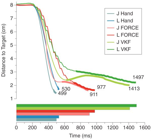
Mean distance to target. Top—the distance (cm) of the arm to the target at each time point averaged across all trials and reach directions for both monkeys. The thicker line is the duration between the first time the monkey acquired the target and the final time the monkey acquired the target. Light blue and blue show monkey J's and L's native hand performance. Light red and red show the FORCE decoder's performance for monkeys J and L in BMI mode. Light green and green show the VKF's performance for monkeys J and L in BMI mode. Bottom—the average last acquire times for both monkeys under all three conditions. Average last acquire time measures how long on average it takes the monkey to complete the task.
Across reach directions and trials, the monkeys took different amounts of time to complete the reaches. The histograms for the average time to reach the target are shown in figure 4. This is the time it took for a monkey to successfully acquire and hold a target without leaving the target box, minus the mandatory hold period of 500 ms, averaged across all trials. For both monkeys, the average acquired time histograms are more skewed toward shorter times for the FORCE decoder in comparison to the VKF.
Figure 4.
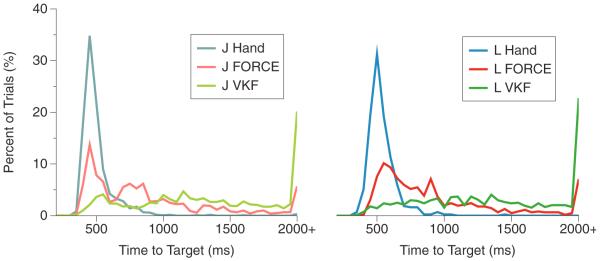
Average acquire time histograms. Left—the histograms of average acquire time (ms), the time it took the monkey to complete a successful trial, across all trials for monkey J. All trials with acquire times greater than 2000 ms are shown at `2000+' ms. (Light blue/native arm, light red/FORCE decoder and light green/VKF). Right—the histograms of average acquire time across all trials for monkey L (blue/native arm, red/FORCE decoder and green/VKF).
One feature of the FORCE decoder is the potential for more accurate kinematics profiles. In the left panel of figure 5, we show the speed profiles for monkey J with native hand (light blue), FORCE decoder in BMI mode (light red) and the VKF in BMI mode (light green). These speed profiles show the cursor speed (the magnitude of the velocity vector), averaged over trials at each time point. The right panel shows the same data for monkey L. These data show that the FORCE decoder was both faster during the initial attempt toward the target (just before 400 ms) and also slowed down more quickly (around 550 ms) as the target was acquired. While not as strong, this pattern also holds for monkey L (right panel, blue/hand, red/FORCE decoder, green/VKF).
Figure 5.
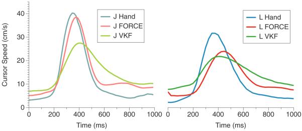
Mean cursor speed. Left—the mean cursor speed (cm s−1), the magnitude of the velocity of the cursor, for monkey J after target onset. Light blue shows monkey J's native hand speed. Light red shows the speed of the cursor with the FORCE decoder in BMI mode. Light green shows the mean cursor speed during operation of the VKF in BMI mode. Right: same as the left panel, but for monkey L (blue/hand, red/FORCE, green/VKF).
Finally, we assessed whether or not a FORCE decoder that was trained on center-out reaches could generalize to a task more difficult than center-out reaches. To test this, we used the FORCE decoder on a moderately more difficult task, known as the pinball task. Briefly, the pinball task uses randomized targets, where the starting position is the last target position and the next target is randomized somewhere within the workspace. To be considered a successful trial, we again enforced a 500 ms hold time of the cursor on the target. We allowed monkey J to continue working on the pinball task until he chose to stop. The results are shown in figure 6. For comparison, in blue is monkey J's native arm performance as measured by the hit rate, or successful targets per minute, over a time period of just over an hour from a separate day (all experimental parameters were the same). In light red, we show the performance of the FORCE decoder. Native arm performance at this task was about 52 targets per minute, while the FORCE decoder was about 37 targets per minute. We were unable to get monkey J to work with the VKF for long enough to take meaningful data with the pinball task, presumably because the VKF's relatively poor control offers too challenging a task for the monkey to use over an extended period of time. In summary, these data show that the FORCE decoder was able to operate constantly and effectively for over an hour on a task that was more general than the task on which the monkey was trained. This task was not attempted with monkey L.
Figure 6.
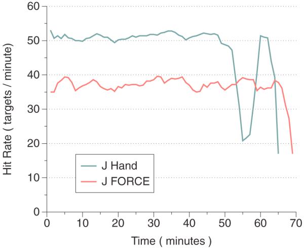
Generalization of the FORCE decoder. The decoder was trained on center-out 8 reaches and then the task was switched to the pinball task. The hit rate, which is the number of successful target acquisitions per minute, is shown for monkey J using his native arm (light blue) and in BMI mode with the FORCE decoder (light red). The monkey was able to sustain performance for over an hour on a more general task. Data for the VKF not shown because the monkey would not work with the VKF decoder long enough to take meaningful data.
Discussion
In this study, we introduced the FORCE decoder, which is a type of RNN with limited learning called an ESN trained with the FORCE learning algorithm, for use in cortical BMIs. We showed that the FORCE decoder outperforms the current standard decoder, the VKF, as measured by the time it takes the cursor to successfully reach the target on average (acquired time before a success). The histograms of the time it takes the cursor to get to the target are skewed toward briefer times for the FORCE decoder as compared to the VKF, primarily due to the reduction in `dial-in' time. Also the mean cursor speed for the FORCE decoder more resembled the speed profile of the monkeys' native arms in terms of acceleration, peak velocity and deceleration. Finally, for monkey J we demonstrated that the FORCE decoder trained on center-out reaches generalized to the more difficult pinball task, and did so for over an hour with a steady hit rate.
We found that the FORCE decoder functions better at faster Δt, allowing a neuronal time constant τ to be set such that network dynamics could successfully follow the velocity profiles of the monkeys' cursor kinematics when controlled by their arms. This better matching of decoder kinematics to native arm kinematics is shown clearly for monkey J (figure 5, left panel) when comparing the speed profile of native arm performance to that of the FORCE decoder in BMI mode.
In general, we had more difficulty training a FORCE decoder for monkey L, presumably because monkey L's array contained less information due to fewer well-modulated channels. Note, for example, monkey L's success rate with the VKF decoder (95.3%) versus the FORCE decoder (92.5%). The design choices that led to better performance were to increase the number of RNN neurons to N = 1500 (see table 1) at the expense of faster dynamics, since we had to increase Δt. In so doing, we attempted to squeeze as much information out of the electrode array as possible. Note that for monkey L, the FORCE decoder nevertheless showed a modest increase in the average maximum speed compared to the VKF. Clearly, having a larger network run at smaller Δt is preferable, but each network time step had to complete in a fixed amount of time, necessitating design tradeoffs for real-time application. The speed profiles shown in figure 5 are consistent with design choices emphasizing speed in monkey J and reliable decodes in monkey L.
Another major design choice was the selection of internal connection strength in the network, g, for each monkey. Again, this choice reflects our understanding of the quality of the information in each monkey's array. Since g scales the strength of internal connectivity in the network, a smaller g will more slavishly follow the inputs (g = 0 gives a feed-forward network). On the other hand, if g ≥ 1, a randomly connected RNN will have ongoing, chaotic dynamics when not driven by a strong input. So a larger g, along with appropriately scaled feedback, WFz(t), will allow a FORCE decoder to more easily and meaningfully generate parts of kinematic patterns that are potentially missing in the neural data. Of course, the potential risk is that those kinematics do not generalize well to novel conditions. Clearly, no amount of pattern generation will make up for the total loss of information in the array.
Since our FORCE decoder outputs both velocity and position (though it need not), we experimented with various combinations of velocity and position by changing the relative contribution parameter, β. For a purely positional decode, β = 0, the decode was noisy and the monkeys were easily frustrated. For a purely velocity-based decode, β = 1, the decoded kinematics were smooth, but were subject to some drift that negatively affected performance. Thus, we settled on β = 0.95, which allowed for a smooth, primarily velocity-based decode while incorporating some positional information to keep the cursor more tightly bound to the workspace.
There are some key next steps to investigate as part of further expanding the capabilities of RNNs as BMI decoders. First, we reported an algorithm named ReFIT-KF (recalibrated feedback intention trained Kalman filter) [42–45], which is a model-independent improvement to online BMI that takes advantage of a two-stage aspect of online decoding. It is possible that the FORCE decoder may also benefit from the application of the ReFIT algorithm. Second, the FORCE decoder learns in a continuous manner (online in the machine learning sense, meaning the updates to trained weights are done incrementally through time). Examining whether continuous learning of the weights of a FORCE decoder during online BMI control might lead to better and more robust decoder performance would also be interesting. Finally, it appears possible to make significant progress in the harder problem of training generically configured RNNs [46]. Given our initial results, investigation of new techniques to train generically configured RNNs applied to BMI could prove fruitful.
There are also some implementation questions that will need to be investigated, as part of using RNNs as BMI decoders in the laboratory setting as well as, potentially, in the fully implantable medical-device setting. Like the VKF, the expensive step of computing the state update of a RNN is the matrix-vector multiplication. First, in the laboratory setting a key question is how many neurons an RNN can have and still run in real time. By real time, we mean receiving inputs, computing, and having available at the output of the RNN the answer within some Δt. The time step Δt in this paper is 15 ms and 25 ms for monkey J and monkey L, respectively. Running on a standard xPC (Intel E8600 3.33 GHz, 2GB RAM) we were able to use 1200 neurons for monkey J and and 1500 neurons for monkey L in our RNNs. This bodes well for the laboratory setting as we were able to run, in real time, a sufficient number of neurons to exceed the state-of-the-art performance of the VKF. In future work, more powerful computers will be able to run ever larger number of neurons. Second, in the fully implantable medical-device context [47], key questions are form factor and power. In terms of form factor, RNNs can be implemented with just a few transistors per neuron and routing/weighting circuitry can also be quite lean. Therefore, replacing a Kalman filter or linear filter in current-integrated circuit designs with a RNN should be possible without significant area differences. In terms of power draw, this too should be possible without significant increases. In fact, it may be possible to substantially reduce the power requirements as RNNs can be implemented using neuromorphic design principles which include spiking neural networks and sub-threshold transistor operation [48, 49]. We have recently demonstrated the real-time operation of a decoder with a few thousand spiking neurons (performing Kalman filtering), which is projected to have substantially lower power draw than a Kalman filter with comparable performance implemented in traditional digital circuitry [50, 51].
Supplementary Material
Acknowledgments
We thank M Risch and J Aguayo for surgical assistance and veterinary care, B Otskotsky for IT support, and S Eisensee and E Castaneda for administrative assistance. This work was supported by a Burroughs Welcome Fund Career Awards in the Biomedical Sciences (KVS), the Christopher and Dana Reeve Paralysis Foundation (SIR, KVS), Stanford Graduate Fellowship (JMF), National Science Foundation Graduate Research Fellowships (JMF, JCK), National Science Foundation IGERT Grant 0734683 (SDS), Stanford Medical Scholars Program, HHMI Medical Research Fellows Program, Paul and Daisy Soros Fellowship, Stanford Medical Scientist Training Program (PN), Defense Advanced Research Projects Agency (DARPA) Revolutionizing Prosthetics 2009 N66001-06-C-8005 (KVS), DARPA Reorganization and Plasticity to Accelerate Injury Recovery N66001-10-C-2010 (KVS), US National Institutes of Health (NIH), National Institute of Neurological Disorders and Stroke Collaborative Research in Computational Neuroscience grant R01-NS054283 (KVS) and NIH Director's Pioneer Award 1DP1OD006409 (KVS).
Footnotes
Online supplementary data available from stacks.iop.org/JNE/9/026027/mmedia
FNNs are more commonly known as artificial neural networks (ANN) or multilayer perceptrons (MLP). We use the term feed-forward here to highlight the difference with a RNN.
In the case of i = 1 or m = 1, it is better to choose the weight from a uniform distribution between −1 and 1.
By `online' we mean in this context the presentation of single examples to the network and learning algorithm, to which the network responds and then the parameters are adjusted. This is in opposition to batch-learning algorithms where all the training data are used to make a single, large modification to the parameters. We do not mean online in the BMI sense of closed-loop interaction with the monkey.
References
- [1].Serruya MD, Hatsopoulos NG, Paninski L, Fellows MR, Donoghue JP. Instant neural control of a movement signal. Nature. 2002;416:141–2. doi: 10.1038/416141a. [DOI] [PubMed] [Google Scholar]
- [2].Taylor DM, Tillery SIH, Schwartz AB. Direct cortical control of 3D neuroprosthetic devices. Science. 2002;296:1829–32. doi: 10.1126/science.1070291. [DOI] [PubMed] [Google Scholar]
- [3].Carmena JM, Lebedev MA, Crist RE, O'Doherty JE, Santucci DM, Dimitrov DF, Patil PG, Henriquez CS, Nicolelis MAL. Learning to control a brain–machine interface for reaching and grasping by primates. PLoS Biol. 2003;1:E42. doi: 10.1371/journal.pbio.0000042. [DOI] [PMC free article] [PubMed] [Google Scholar]
- [4].Velliste M, Perel S, Spalding MC, Whitford AS, Schwartz AB. Cortical control of a prosthetic arm for self-feeding. Nature. 2008;453:1098–101. doi: 10.1038/nature06996. [DOI] [PubMed] [Google Scholar]
- [5].Mulliken GH, Musallam S, Andersen RA. Decoding trajectories from posterior parietal cortex ensembles. J. Neurosci. 2008;28:12913–26. doi: 10.1523/JNEUROSCI.1463-08.2008. [DOI] [PMC free article] [PubMed] [Google Scholar]
- [6].Shpigelman L, Lalazar H, Vaadia E. Kernel-ARMA for hand tracking and brain–machine interfacing during 3D motor control. Adv. Neural Inform. Process. Syst. 2009;21:1489–96. [Google Scholar]
- [7].Ganguly K, Carmena JM. Emergence of a stable cortical map for neuroprosthetic control. PLoS Biol. 2009;7:e1000153. doi: 10.1371/journal.pbio.1000153. [DOI] [PMC free article] [PubMed] [Google Scholar]
- [8].Suminski AJ, Tkach DC, Fagg AH, Hatsopoulos NG. Incorporating feedback from multiple sensory modalities enhances brain–machine interface control. J. Neurosci. 2010;30:16777–87. doi: 10.1523/JNEUROSCI.3967-10.2010. [DOI] [PMC free article] [PubMed] [Google Scholar]
- [9].Hochberg LR, Serruya MD, Friehs GM, Mukand JA, Saleh M, Caplan AH, Branner A, Chen D, Penn RD, Donoghue JP. Neuronal ensemble control of prosthetic devices by a human with tetraplegia. Nature. 2006;442:164–71. doi: 10.1038/nature04970. [DOI] [PubMed] [Google Scholar]
- [10].Kim S-P, Simeral JD, Hochberg LR, Donoghue JP, Friehs GM, Black MJ. Point-and-click cursor control with an intracortical neural interface system by humans with tetraplegia. IEEE Trans. Neural Syst. Rehabil. Eng. 2011;19:193–203. doi: 10.1109/TNSRE.2011.2107750. [DOI] [PMC free article] [PubMed] [Google Scholar]
- [11].Kim S-P, Simeral JD, Hochberg LR, Donoghue JP, Black MJ. Neural control of computer cursor velocity by decoding motor cortical spiking activity in humans with tetraplegia. J. Neural Eng. 2008;5:455–76. doi: 10.1088/1741-2560/5/4/010. [DOI] [PMC free article] [PubMed] [Google Scholar]
- [12].Graziano MSA. New insights into motor cortex. Neuron. 2011;71:387–8. doi: 10.1016/j.neuron.2011.07.014. [DOI] [PubMed] [Google Scholar]
- [13].Kalaska JF. From intention to action: motor cortex and the control of reaching movements. Adv. Exp. Med. Biol. 2009;629:139–78. doi: 10.1007/978-0-387-77064-2_8. [DOI] [PubMed] [Google Scholar]
- [14].Churchland MM, Shenoy KV. Temporal complexity and heterogeneity of single-neuron activity in premotor and motor cortex. J. Neurophysiol. 2007;97:4235–57. doi: 10.1152/jn.00095.2007. [DOI] [PubMed] [Google Scholar]
- [15].Scott SH. Optimal feedback control and the neural basis of volitional motor control. Nat. Rev. Neurosci. 2004;5:532–46. doi: 10.1038/nrn1427. [DOI] [PubMed] [Google Scholar]
- [16].Churchland MM, Cunningham JP, Kaufman MT, Ryu SI, Shenoy KV. Cortical preparatory activity: representation of movement or first cog in a dynamical machine? Neuron. 2010;68:387–400. doi: 10.1016/j.neuron.2010.09.015. [DOI] [PMC free article] [PubMed] [Google Scholar]
- [17].Afshar A, Santhanam G, Byron MY, Ryu SI, Sahani M, Shenoy KV. Single-trial neural correlates of arm movement preparation. Neuron. 2011;71:555–64. doi: 10.1016/j.neuron.2011.05.047. [DOI] [PMC free article] [PubMed] [Google Scholar]
- [18].Scott SH. Inconvenient truths about neural processing in primary motor cortex. J. Physiol. 2008;586:1217–24. doi: 10.1113/jphysiol.2007.146068. [DOI] [PMC free article] [PubMed] [Google Scholar]
- [19].Bishop CM. Pattern Recognition and Machine Learning. Springer; Berlin: 2006. [Google Scholar]
- [20].Taylor G, Hinton G, Roweis S. Modeling human motion using binary latent variables. Adv. Neural Inform. Process. Syst. 2007;19:1345–52. [Google Scholar]
- [21].Chapin JK, Moxon KA, Markowitz RS, Nicolelis MA. Real-time control of a robot arm using simultaneously recorded neurons in the motor cortex. Nature Neurosci. 1999;2:664–70. doi: 10.1038/10223. [DOI] [PubMed] [Google Scholar]
- [22].Wessberg J, Stambaugh CR, Kralik JD, Beck PD, Laubach M, Chapin JK, Kim J, Biggs SJ, Srinivasan MA, Nicolelis MA. Real-time prediction of hand trajectory by ensembles of cortical neurons in primates. Nature. 2000;408:361–5. doi: 10.1038/35042582. [DOI] [PubMed] [Google Scholar]
- [23].Rumelhart D, Hinton G, Williams R. Learning internal representations by error propagation. Parallel Distrib. Process. 1985;1:319–62. [Google Scholar]
- [24].Williams R, Zipser D. A learning algorithm for continually running fully recurrent neural networks. Neural Comput. 1989;1:270–80. [Google Scholar]
- [25].Doya K. Bifurcations in the learning of recurrent neural networks. Proc. IEEE Int. Symp. Circuits and Systems: ISCAS '92. 1992;6:2777–80. [Google Scholar]
- [26].Bengio Y, Simard P, Frasconi P. Learning long-term dependencies with gradient descent is difficult. IEEE Trans. Neural Netw. 1994;5:157–66. doi: 10.1109/72.279181. [DOI] [PubMed] [Google Scholar]
- [27].Fetz EE. Real-time control of a robotic arm by neuronal ensembles. Nature Neurosci. 1999;2:583–4. doi: 10.1038/10131. [DOI] [PubMed] [Google Scholar]
- [28].Fetz E. Are movement parameters recognizably coded in the activity of single neurons? Behav. Brain Sci. 1992;15:679–90. [Google Scholar]
- [29].Maier MA, Shupe LE, Fetz EE. Recurrent neural networks of integrate-and-fire cells simulating short-term memory and wrist movement tasks derived from continuous dynamic networks. J. Physiol. Paris. 2003;97:601–12. doi: 10.1016/j.jphysparis.2004.01.017. [DOI] [PubMed] [Google Scholar]
- [30].Maier MA, Shupe LE, Fetz EE. Dynamic neural network models of the premotoneuronal circuitry controlling wrist movements in primates. J. Comput. Neurosci. 2005;19:125–46. doi: 10.1007/s10827-005-0899-5. [DOI] [PubMed] [Google Scholar]
- [31].Jaeger H, Haas H. Harnessing nonlinearity: predicting chaotic systems and saving energy in wireless communication. Science. 2004;304:78–80. doi: 10.1126/science.1091277. [DOI] [PubMed] [Google Scholar]
- [32].Sussillo D, Abbott LF. Generating coherent patterns of activity from chaotic neural networks. Neuron. 2009;63:544–57. doi: 10.1016/j.neuron.2009.07.018. [DOI] [PMC free article] [PubMed] [Google Scholar]
- [33].Sanchez JC, Erdogmus D, Nicolelis MAL, Wessberg J, Principe JC. Interpreting spatial and temporal neural activity through a recurrent neural network brain–machine interface. IEEE Trans. Neural Syst. Rehabil. Eng. 2005;13:213–9. doi: 10.1109/TNSRE.2005.847382. [DOI] [PubMed] [Google Scholar]
- [34].Gunduz A, Sanchez JC, Carney PR, Principe JC. Mapping broadband electrocorticographic recordings to two-dimensional hand trajectories in humans motor control features. Neural Netw. 2009;22:1257–70. doi: 10.1016/j.neunet.2009.06.036. [DOI] [PubMed] [Google Scholar]
- [35].Cunningham JP, Nuyujukian P, Gilja V, Chestek CA, Ryu SI, Shenoy KV. A closed-loop human simulator for investigating the role of feedback control in brain-machine interfaces. J. Neurophys. 2011;105:1932–49. doi: 10.1152/jn.00503.2010. [DOI] [PMC free article] [PubMed] [Google Scholar]
- [36].Chestek CA. Long-term stability of neural prosthetic control signals from silicon cortical arrays in rhesus macaque motor cortex. J. Neural Eng. 2011;8:045005. doi: 10.1088/1741-2560/8/4/045005. [DOI] [PMC free article] [PubMed] [Google Scholar]
- [37].Santhanam G, Ryu SI, Byron MY, Afshar A, Shenoy KV, et al. A high-performance brain–computer interface. Nature. 2006;442:195–8. doi: 10.1038/nature04968. [DOI] [PubMed] [Google Scholar]
- [38].Ryu SI, Shenoy KV. Human cortical prostheses: lost in translation? Neurosurg. Focus. 2009;27:5. doi: 10.3171/2009.4.FOCUS0987. [DOI] [PMC free article] [PubMed] [Google Scholar]
- [39].Churchland MM, Byron MY, Sahani M, Shenoy KV. Techniques for extracting single-trial activity patterns from large-scale neural recordings. Curr. Opin. Neurobiol. 2007;17:609–18. doi: 10.1016/j.conb.2007.11.001. [DOI] [PMC free article] [PubMed] [Google Scholar]
- [40].Haykin S. Adaptive Filter Theory. 4th edn Prentice-Hall; Englewood Cliffs, NJ: 2001. [Google Scholar]
- [41].Simeral JD, Kim SP, Black MJ, Donoghue J, Hochberg L. Neural control of cursor trajectory and click by a human with tetraplegia 1000 days after implant of an intracortical microelectrode array. J. Neural Eng. 2011;8:025027. doi: 10.1088/1741-2560/8/2/025027. [DOI] [PMC free article] [PubMed] [Google Scholar]
- [42].Nuyujukian P, Fan JM, Kao JC, Ryu SI, Shenoy KV. Towards robust performance and streamlined training of cortically-controlled brain–machine interfaces. Program No 142.02: Neuroscience Meeting Planner; Washington, DC: Society for Neuroscience; 2011. [Google Scholar]
- [43].Gilja V, Nuyujukian P, Chestek CA, Cunningham JP, Fan JM, Yu BM, Ryu SI, Shenoy KV. A high-performance continuous cortically-controlled prosthesis enabled by feedback control design. Program No 20.7.2010: Neuroscience Meeting Planner.2010. [Google Scholar]
- [44].Nuyujukian P, Gilja V, Chestek CA, Cunningham JP, Fan JM, Yu BM, Ryu SI, Shenoy KV. Generalization and robustness of a continuous cortically-controlled prosthesis enabled by feedback control design. Program No 20.7.2010: Neuroscience Meeting Planner; San Diego, CA: Society for Neuroscience; 2010. [Google Scholar]
- [45].Gilja V, Nuyujukian P, Chestek CA, Cunningham JP, Yu BM, Ryu SI, Shenoy KV. High-performance continuous neural cursor control enabled by a feedback control perspective. Computational and Systems Neuroscience (COSYNE). Frontiers in Neuroscience: Conference Abstract (Salt Lake City, UT).2010. [Google Scholar]
- [46].Martens J, Sutskever I. Learning recurrent neural networks with Hessian-free optimization. Proc. 28th Int. Conf. on Machine Learning.2011. [Google Scholar]
- [47].Nurmikko AV, et al. Listening to brain microcircuits for interfacing with external world-progress in wireless implantable microelectronic neuroengineering devices: experimental systems are described for electrical recording in the brain using multiple microelectrodes and short range implantable or wearable broadcasting units. Proc. IEEE. Inst. Electr. Electr. Eng. 2010;98:375–88. doi: 10.1109/JPROC.2009.2038949. [DOI] [PMC free article] [PubMed] [Google Scholar]
- [48].Boahen K. Neuromorphic microchips. Sci. Am. 2005;292:56–63. doi: 10.1038/scientificamerican0505-56. [DOI] [PubMed] [Google Scholar]
- [49].Arthur JV, Kwabena BA. Silicon-neuron design: a dynamical systems approach. IEEE Trans. Circuits Syst. 2011;58:1034–43. doi: 10.1109/TCSI.2010.2089556. [DOI] [PMC free article] [PubMed] [Google Scholar]
- [50].Dethier J, Nuyujukian P, Eliasmith C, Stewart T, Elasaad S, Shenoy KV. Advances in Neural Information Processing Systems (NIPS) Vol. 24. MIT Press; Cambridge, MA: 2011. A brain–machine interface operating with a real-time spiking neural network control algorithm. http://hdl.handle.net/2268/100574. [PMC free article] [PubMed] [Google Scholar]
- [51].Dethier J, Gilja V, Nuyujukian P, Elassaad S, Shenoy KV, Boahen K. Spiking neural network decoder for brain–machine interfaces. 5th Int. IEEE EMBS Conf. on Neural Engineering; 2011. [DOI] [PMC free article] [PubMed] [Google Scholar]
Associated Data
This section collects any data citations, data availability statements, or supplementary materials included in this article.