An integrative variant analysis pipeline for accurate genotype/haplotype inference in population NGS data

Abstract

Next-generation sequencing is a powerful approach for discovering genetic variation. Sensitive variant calling and haplotype inference from population sequencing data remain challenging. We describe methods for high-quality discovery, genotyping, and phasing of SNPs for low-coverage (approximately 5×) sequencing of populations, implemented in a pipeline called SNPTools. Our pipeline contains several innovations that specifically address challenges caused by low-coverage population sequencing: (1) effective base depth (EBD), a nonparametric statistic that enables more accurate statistical modeling of sequencing data; (2) variance ratio scoring, a variance-based statistic that discovers polymorphic loci with high sensitivity and specificity; and (3) BAM-specific binomial mixture modeling (BBMM), a clustering algorithm that generates robust genotype likelihoods from heterogeneous sequencing data. Last, we develop an imputation engine that refines raw genotype likelihoods to produce high-quality phased genotypes/haplotypes. Designed for large population studies, SNPTools' input/output (I/O) and storage aware design leads to improved computing performance on large sequencing data sets. We apply SNPTools to the International 1000 Genomes Project (1000G) Phase 1 low-coverage data set and obtain genotyping accuracy comparable to that of SNP microarray.

Next-generation sequencing technologies (NGS) are rapidly becoming a desirable choice for population-level genomic studies. Until high-coverage sequencing becomes affordable for large cohort interrogation, study designs that aggregate NGS data across thousands of subjects are compelling (Li et al. 2011). Low-coverage population (approximately 3×–5× coverage over the whole genome) sequencing strategy aims to achieve both high-sensitivity population-level variant discovery and high-accuracy genotyping by utilizing redundancy of reads at loci across multiple samples. Borrowing strength across multiple samples improves identification of common and low-frequency (minor allele frequency, >0.5%–1%) genetic variants (The 1000 Genomes Project Consortium 2010). Linkage disequilibrium (LD) between variants allows for genotype imputation to improve sensitivity and specificity (Nielsen et al. 2011). For example, if two SNPs are tightly linked in the population (r² = 1), then their respective read depth can be shared/summed to obtain much more accurate genotype calls at both sites (Carlson et al. 2004; International HapMap Consortium 2005; Duitama et al. 2011; Le and Durbin 2011). This strategy was initially demonstrated by Liti et al. (2009) and on a large scale in the 1000G Pilot (The 1000 Genomes Project Consortium 2010).

Analytical challenges in low-coverage genome sequencing data had not been fully addressed by most SNP calling pipelines. For example, tools such as SOAPsnp (Li et al. 2008) detect SNP sites on a sample by sample basis. As a result, for a population-based study, each sample is evaluated independently and the analyzed data are then aggregated. These methods also tend to apply simple heuristics to read level information such as mapping and base quality (Li et al. 2008). For example, a common cut off is the phred-type quality score of Q20. The application of simple heuristics does not measurably impact high-coverage genome studies due to the high number of reads at each position (Nielsen et al. 2011); however, filtering for parameters such as mapping and base quality reduces the power to detect variants in low-coverage studies because of the limited number of reads at each locus. In addition, simple heuristics are difficult to generalize to new data due to sequencing platform, reagent, and mapping algorithm heterogeneity (Harismendy et al. 2009; Suzuki et al. 2011).

We devise an integrative pipeline, “SNPTools,” which achieves high-quality (1) variant site discovery, (2) genotype likelihood (GL) estimation, and (3) genotype/haplotype inference from population NGS data. The pipeline, in particular, introduces two new constructs for low-coverage data: (1) effective base depth (EBD) as a pseudo-count for read depth and (2) BAM-specific binomial mixture model (BBMM), which calculates GLs. The SNPTools pipeline demonstrates high performance when dealing with low-coverage (approximately 2×–6× per sample) data that are collected from heterogeneous platforms.

Results

SNPTools is organized by functionality into four modules (Fig. 1):

Figure 1.

Overview of the SNPTools Pipeline. The SNPTools pipeline utilizes binary sequence map (BAM) files and then processes them through four modular steps: calculation of effective base depth (EBD), SNP site discovery, BAM-specific binomial mixture modeling (BBMM) to calculate genotype likelihoods, and genotype and haplotype imputation.

1. EBD calculation: It summarizes mapping and base quality information to improve computational performance and reduce storage space.

2. SNP site discovery: The variance ratio statistic utilizes EBD information to provide high-quality SNP variant calls. Optional heuristic filters can be applied subsequently to further improve the specificity of these calls.

3. GL estimation: BBMM incorporates EBD to generate GLs at discovered variant sites. BAM-specific parameter estimation allows this algorithm to overcome data heterogeneity due to platforms, reference bias (from mapping or capture), and low-quality data.

4. Genotype/haplotype imputation: A “constrained Li-Stephens” population haplotype sampling schema that is based on genetic coalescence reduces computational burden when dealing with thousands of samples in cohort sequencing projects.

The variants from this pipeline are provided as phased genotype results in the variant calling format (VCF) (Fig. 1). Users have the option to apply the pipeline as an integrated NGS variant caller or to apply individual components to produce intermediate results. These individual modules and their intermediate results are compatible with a number of available tools. For example, if variant sites are discovered using SAMtools (Li et al. 2009), SNPTools can be applied to generate highly accurate GLs. The GLs can subsequently be used for genotype and haplotype inference through SNPTools' imputation algorithm or others such as Beagle (Browning and Browning 2007).

EBD summarizes read depth information after recalibration with base qualities and mapping qualities

Quality indicators such as base quality and mapping/alignment quality scores have been utilized in NGS to improve sensitivity and specificity in variant calling (DePristo et al. 2011; Li 2011a). These quality scores are under continuous improvement and are regularly recalibrated by different tools to attempt to accurately reflect the true underlying sequence qualities (Li 2011b) and are often used by different heuristic approaches for SNP discovery. For example, one may choose to remove all bases with a phred-type quality score below Q20 and reads with mapping quality score of zero. This approach is suitable for high-coverage studies (Koboldt et al. 2009; Nielsen et al. 2011); however, it can result in a pronounced reduction in sensitivity in data where average coverage is approximately 3×–5× coverage per individual.

To maximize the usable read depth information, we calculate a sample and locus-specific pseudo-count, EBD. For each genomic position, s, there are K_s number of reads covering the site. An EBD value is calculated for each nucleotide (A, C, G, and T) by weighing each individual read, k, with its base quality and mapping quality. Thus for each sample and locus, we calculate four EBD values, one for each nucleotide (Equation 1) (for derivation, see Supplemental Material):

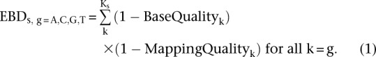In this framework, the maximum EBD value for a single read is one (base quality and mapping quality are defined as the probability of an error). This occurs when both base quality and mapping quality are high. If there is no read level evidence for a given alternative nucleotide, it is assigned a value of zero. SNPTools utilizes EBD as the underlying read depth throughout our pipeline. For example, EBD is used in SNP site discovery and in GL estimation and is used in all derivations in this manuscript.

Variance ratio statistic–based SNP site discovery

A major challenge in variant site discovery from low-coverage data stems from the relatively high error rate (∼1%) that originates from sequencing and mapping. These errors can introduce false allele counts that confound calls for the true alternative base(s). Rare variants with allele frequency <5% in low-coverage studies can be difficult to differentiate from this background noise due to the low allele counts in the population. To improve identification of variants, SNPTools utilizes a two-step SNP site discovery process that first aggregates reads from all the sequenced samples in order to identify the alternative alleles and then applies a statistical test to evaluate whether they are true variant alleles instead of sequencing errors.

To identify and select a possible alternative allele, we compute four population-level EBD values for each site, by summing the squared EBD values for each of the nucleotides over all samples i = 1,…,I. The reference allele is defined by human genome build hg19 (GRSCh37). We select the nonreference allele (of the remaining 3 nucleotides) that has the greatest squared EBD evidence as the alternative allele (for details, see Supplemental Material).

It is important to note that we are employing a biallelic assumption by selecting only a single alternative nucleotide. While there is evidence that poor modeling of triallelic alleles may result in false negatives (Le and Durbin 2011), we use a biallelic assumption because triallelic loci only comprise ∼0.2% of all SNPs (Hodgkinson and Eyre-Walker 2010). While this limits our ability to detect multiallelic variant sites segregating in the population, it nonetheless reduces by ∼60% the number of alternative bases that are called due to sequencing errors. Further, a biallelic assumption simplifies downstream analytical steps and reduces the computational cost in large-scale imputation.

After having selected a candidate alternative allele, we utilize the variance ratio statistic to evaluate the existence of an alternative allele. The numerator of the variance ratio statistic calculates the excess variation above the null hypothesis, i.e., the extra-binomial variation for a given site. For example, if reads for alternative alleles cluster among a few samples, the extra-binomial variation will be high when compared to a situation where the alternative alleles are distributed relatively evenly across samples. The latter case, the null hypothesis, describes the likely distribution when alternative alleles are generated by sequencing errors.

The first term in the numerator is the sum of the estimated variance in the observed data over all individuals. This is calculated by summing the square of the difference between the observed EBD of the alternative allele and the expected EBD of the alternative allele in the population. The second term is the Bernoulli variance for the population, assuming a null hypothesis (Equation 2). We omit the site level index, s, for readability:

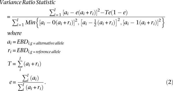To enhance our ability to detect true sites of genetic variation, we take advantage of the genotype property of biallelic SNPs. For a SNP, there are only three genotypes with corresponding binomial parameters (0, 0.5, and 1 for Ref/Ref, Ref/Alt, and Alt/Alt, respectively). We construct a goodness-of-fit test that sums over all samples the squared difference in the observed EBD for the alternative allele and the expected EBD for each of the three genotypes. The smallest sum provides the best fit for a given genotype. Placing the goodness of fit test in the denominator has the effect of maximizing the variance ratio statistic for true-positive sites (Equation 2). Thus the variance ratio statistic computes a ratio between the extra-binomial variation and the best genotype fit. Sites with high levels of extra-binomial variation and a best genotype model will have the highest computed statistic, while sites with low extra-binomial variation or no genotype fit will have the lowest statistic. We rank the candidate sites by their computed variance ratio statistic (for derivation, see Supplemental Material).

Estimation of GLs by BBMM

As evidence for alternative alleles in low-coverage sequencing data is limited, it is difficult to calculate the data likelihood for a particular genotype. Small amounts of variability in mapping and base quality may result in lower-confidence GL. This variability can also be exacerbated by operational heterogeneity between sequencing centers and between sequencing runs. For example, sequencing centers may vary in sequencers (platforms and versions), aligners, and other operational parameters, while sequencing runs may vary in reagent composition or by operator. If summed together, this variability will decrease the signal-to-noise ratio. In order to overcome the operational heterogeneity common to large-scale sequencing projects with several thousand BAMs such as the 1000G and projects like GO Exome Sequencing Project (ESP) (http://evs.gs.washington.edu/EVS/), we developed BBMM, which accurately estimates GLs for putative variant sites by modeling intra-BAM variability. The millions of putative SNP sites within each BAM provide SNPTools a large data set from which it is possible to perform accurate BAM-specific genotype class parameter estimation (Fig. 2A). These parameters are then used to calculate the GL in light of the EBD evidence for each putative site.

Figure 2.

Illustration of the BBMM. (A) BBMM models each BAM as a mixture of three binomials that represent the three genotypes classes (rr = Ref/Ref, ra = Ref/Alt, and aa = Alt/Alt). Each of these classes has a class-specific binomial probability, p_v which is defined as the probability of a reference read for a given genotype. BBMM estimates the parameters for each BAM by pooling data from all variant sites (approximately 34 million candidate sites that we discovered in the 1000G). (B–D) To qualitatively view the cluster assignment for each site, we compute an expected number of reference alleles by multiplying the genotype likelihood (GL) for each genotype by the number of reference alleles. We find that BBMM is able to cluster the genotypes for Illumina, SOLiD, and 454 sequencers. As representative samples, we plot HG00096 sequenced with the Illumina platform and aligned using BWA (B), HG00076 sequenced with the SOLiD platform and aligned using BFAST (C), and NA07347 sequenced by the 454 platform and aligned using SSAHA (D).

For each sample i, we model the BAM as a mixture of three binomials that each represent the three genotype classes rr = Ref/Ref, ra = Ref/Alt, and aa = Alt/Alt. Each of the three genotype classes has a weight coefficient w_v, where the sum of the weights is equal to 1, and a binomial probability p_v, which is defined as the probability of a reference read. If sequencing was error free, the binomial probability would be equal to 1, 0.5, and 0 for ; in practice, this parameter deviates from ideal values due to sequencing variability. To estimate the value of these parameters, we employ the expectation-maximization (EM) algorithm (Dempster et al. 1977; Bishop 2006).

We initialize the EM algorithm by introducing a binary three-dimensional latent variable , which assigns each site to a genotype class. This variable takes a 1 of V representation; i.e., if and only if the site is in genotype class (Bishop 2006). The EM algorithm allows us to iteratively compute the maximum likelihood expectation (MLE) of the latent variables and the unknown parameters. We start the E-step by initializing the parameters {} and computing the expectation of with respect to the initial parameters and the data {}. For the M-step, the updated parameters maximize the joint data likelihood of {} (for details, see Supplemental Material).

After convergence, we use these parameters to calculate the GL at each site given the genotype class (Equation 3):

A binomial mixture is a flexible continuous distribution composed of three parametric densities.

Genotype/haplotype inference via imputation using a “constrained Li-Stephens” algorithm

For most sites, utilizing a maximum likelihood method for genotyping will result in low-accuracy genotypes, particularly in heterozygous calls due to the dearth of coverage. Imputation is thus an integral part of accurate genotype calling in low-coverage sequencing projects (Li et al. 2011; Nielsen et al. 2011). Accurate phased genotype imputation requires capturing LD patterns that result from recombination (Scheet and Stephens 2006).

Many imputation algorithms are based on work on coalescent recombination processes (Kingman 1982; Hudson 1983). Hidden Markov model (HMM) block-based cluster models divide the genome into predetermined segments of high LD based on known recombination rates and allow cluster assignment to shift only along these boundaries (Greenspan and Geiger 2004). This approach, while computationally efficient, cannot accommodate more complex patterns of LD. The PAC model of Li and Stephens (2003), which underlies the Markov chain-based PHASE software, flexibly accommodates patterns of LD by conditioning the joint distribution of sampled haplotypes on the recombination rate. Additional HMM-based haplotype estimation packages such as fast PHASE (Scheet and Stephens 2006) and MaCH (Li et al. 2010) share these underlying features; i.e., these models utilize sampled haplotypes as a mosaic of a set of population haplotypes but improve computational time.

Our imputation method also derives from the genetic coalescence-based method. However direct application of the Li and Stephens (2003) method is computationally expensive; the estimation of a multihaplotype mosaic model by HMM is demanding due to the large number of hidden states that scales with the number of samples I [O (I²) states and O (I⁴) transitions]. In our model, the “constrained Li-Stephens” method, we use a haplotype template-sampling scheme that constrains the number of parental haplotypes to only four during the HMM. This tremendously eases the computational burden by allowing us to sample in constant time [from O (I⁴) to ∼O (I) time].

To begin the phasing and imputation process, we first initialize haplotypes for each individual by randomly generating haplotypes given the set of observed GL. We then iterate the following two steps to produce accurate phased genotypes. (1) For each sample H_i, we search for a set of four “parental” haplotypes, H_i*, by proposing haplotypes from the sample population based on observed GLs for each sample. We accept and reject it according to a Metropolis Hastings (M-H) acceptance criterion (see Supplemental Material). We repeat the M-H sampler a fixed number of times. (2) Once the set of four parental haplotypes are selected, we refine the sample's haplotype H_i, using a four-state HMM where the sample haplotype is a mosaic combination of the four parental haplotypes. We repeat the above procedure defined for all samples until convergence.

Applying SNPTools to obtain high-quality results from the 1000 Genomes Low-Coverage NGS data

The 1000G low-coverage component (LowCov) sequenced 1092 individuals from 14 ethnicities at an average coverage of ∼3×–6× (Methods) (Abecasis et al. 2012). The data were produced at nine different sequencing centers using three NGS platforms, Illumina, SOLiD, or Roche 454 (Methods). The alignments were produced using BWA (Li and Durbin 2009), BFAST (Homer et al. 2009), and SSAHA (Ning et al. 2001) for different platforms (Illumina, SOLiD, and Roche 454), respectively. This level of heterogeneity reflects the reality of many large cohort disease studies; therefore, the challenges of the 1000G can be generalized and transferred to other ongoing large-scale studies as well. We have applied SNPTools to the 1000G LowCov data as a proof of principle and obtained high-quality results.

Variance ratio statistic produces candidate SNP sites with high sensitivity and specificity

Using a cut-off of 1.5 for our variance ratio statistic (see Supplemental Material), we generated an autosomal unfiltered SNP site list with 34,656,295 candidate SNP sites. These sites had an overall SNP transition/transversion ratio (Ti/Tv) of 2.11, a value consistent with genome-wide expectations, ratios found using GATK (DePristo et al. 2011), and values found in the 1000G Pilot (Supplement Table S3; The 1000 Genomes Project Consortium 2010). The Ti/Tv ratio is an important metric for assessing the specificity of new SNP calls, with the caveat that uncertainties in Ti/Tv ratio limit its interpretation in cases of minor differences in Ti/Tv ratios (<0.05) (DePristo et al. 2011). We evaluated sensitivity and specificity of the unfiltered call set using sites on Illumina 2.5M OMNI SNP microarray (Methods). We compare to the microarray because it is an orthogonal technology to NGS (Supplemental Table 3). Sensitivity for polymorphic sites was 97.9% (2,138,395 of 2,183,344 polymorphic OMNI SNP sites were discovered). The false-discovery rate (FDR) was 1.95% (1946 of 99,817 monomorphic OMNI SNP sites were falsely discovered), similar to the rates found by QCALL in the 1000G Pilot CEU data (Supplemental Table 3; Le and Durbin 2011).

To improve SNP specificity, we applied the following optional heuristics: (1) maximum population read depth, (2) minimum population read depth, (3) strand bias as tested by a 2 × 2 contingency table, and (4) position bias to the unfiltered SNP site. These criteria effectively removed false-positive sites but at the cost of reducing sensitivity (Methods; Supplemental Table 1). After application of these heuristics, 5.5% of the originally discovered sites were removed. The remaining 32,737,954 SNP sites had an overall Ti/Tv from 2.11–2.15. This call set included 7.2M previously discovered SNPs (ascertained by comparing to dbSNP129) and 25.6M novel SNPs (Fig. 3A). As expected, the vast majority of novel SNPs had minor allele frequency (MAF) < 1%, with the majority of the SNPs with MAF < 0.25% (Fig. 3B). The Ti/Tv ratio for known and novel sites of 2.17 and 2.15, respectively, was comparable and indicated a high-quality discovery process (Fig. 3C). The false-positive rate was reduced to 1.29% (1284 of 99,817 monomorphic OMNI SNP sites were falsely discovered), a reduction of ∼30% in FDR when compared to the unfiltered call set. However the sensitivity was also reduced by 4.3% to 93.6% (Supplemental Table S2). The removed sites had a Ti/Tv ratio ranging from 1.30–1.74, a large deviation from genome-wide expectations and an indicator that these were largely false positive sites (Supplemental Table S3).

Figure 3.

SNP statistics for sites discovered in 1000G PHASE1 with SNPTools. SNP sites were discovered using the variance ratio statistic. The unfiltered autosomal site list was composed of 34,656,295 candidate SNP sites, with an average Ti/Tv ratio of 2.11. SNPs were filtered using four criteria (Supplemental Material) to produce a final list of 32,737,954 SNPs with a Ti/Tv ratio of 2.15. (A) We found that 78.3% of the ∼32.7 million SNP were novel when evaluated with dbSNP 129. These novel sites had a Ti/Tv ratio of 2.15, which was comparable to the Ti/Tv of known sites, 2.17. (B) The site frequency spectrum of our discovered SNPs reveals that most novel SNPs were rare with MAF < 0.5%. (C) We provide discovery statistics for Chr20 and for the whole genome. Known SNPs are defined as being present in dbSNP129. SNPTools had a low false-discovery rate of 1284 sites out of 99,817 monomorphic OMNI sites.

To validate the SNP discovery methods, the 1000G Consortium also conducted a SNP validation of 300 low-coverage sites in eight samples selected from the variant quality score recalibration (VQSR) consensus list version 2b (Methods). This site list was pooled from the SNP site lists of five different sequencing centers, which includes BCM SNPTools. The SNPTools filtered site list overlapped 297 of these randomly selected 300 selected sites. The three sites not included in our call set were singleton sites. By use of PCR, this study showed an overall confirmation rate of 98.2%, with 100% confirmation of sites with >1% MAF, all of which were included in the SNPTools call set. Although a small sample size, this study provides further support for the quality of our site list (Methods).

To further investigate the false-negative rate of the SNPTools discovery process, we compare our SNP discovery against the 363,034 sites discovered in the Phase 1 exome consensus. Sites discovered in the exome project benefit from the high coverage provided by exome capture and sequencing. This comparison provides an upper bound on the discovery rate. We found that our SNPTools discovery process was able to discover >43.6% (158,431) of all SNPs discovered in the Phase 1 exome project, with 96.7% sensitivity for SNPs with MAF > 1.0%. Of the undetected SNPs, 90.3% had a MAF < 0.10% (i.e., singletons, doubletons), while 99.1% had MAF < 0.50%. This mainly reflects the limitations of low-coverage sequencing and not SNPTools.

High-quality GLs were generated using BBMM

The BBMM algorithm overcomes platform, technology, and alignment heterogeneity by estimating BAM-specific parameters for the VQSR2b sites that were discovered in the 1000G Phase 1 (Methods). BBMM generates GLs by separately modeling each BAM over all VQSR2b sites as a mixture of three binomials (Fig. 2A). We plot the expected number of reference alleles for all sites for samples HG00096, HG00076, and NA07347 as examples. These samples were sequenced using the Illumina, SOLiD, and 454 platforms, respectively. Although these platforms utilize different technologies for sequencing, Illumina (sequencing by bridge amplification), SOLiD (bead and ligase based sequencing), and 454 (pyrosequencing) (Shendure and Ji 2008), we nevertheless found that BBMM is able to cluster the three different genotypes Ref/Ref, Ref/Alt, and Alt/Alt for the three. However the clustering between genotype groupings appears more distinct for the Illumina and SOLiD sequencers than for 454, particularly for Ref/Alt genotypes (Fig. 2B–D).

We further examine the classification of EBD into the three-genotype classes by evaluating the ability of raw GL to estimate genotypes using maximum likelihood. While genotypes estimated via imputation are more accurate, we compare chromosome 20 genotypes estimated from SNPTools GL using maximum likelihood and compared them to OMNI genotypes to identify a maximum error rate for genotype accuracy. We found that the genotype discordance rates over all samples for Ref/Ref, Ref/Alt, and Alt/Alt to be 0.4%, 28.2%, and 1.1%, respectively. The lower accuracy in heterozygous estimates is expected as the low-coverage nature of the project results in a high probability that only one of the two haplotypes have been sampled at a specific site. For example, for a heterozygous site with 5× coverage, there is an 18.75% (binomial distribution) chance that only zero or one alternative allele is sampled. This results in underrepresentation of heterozygous genotypes when using maximum likelihood variant calling. As suggested by Figure 2, B through D, there were sequencer-specific differences in genotype accuracy when estimated using maximum likelihood. Illumina had an average discordance rate of 0.43%, 27.0%, and 0.92% for Ref/Ref, Ref/Alt, and Alt/Alt alleles; however, SOLiD had discordance rates of 0.26%, 35.24%, and 2.70%, while 454 had discordance rates of 0.26%, 47.52%, and 1.13%. These differences were likely due to reference bias in SOLiD and comparatively lower read coverage in Roche 454.

To evaluate clustering quality in BBMM, we plotted the binomial probability, p_rr, (Ref/Ref) and p_aa, (Alt/Alt) for all samples (Figure 4A–D). As the binomial probability can reflect the sequencing variability in a BAM, we expect samples to have high correlation between the binomial probabilities. Although we find some variation between samples, binomial probabilities for these genotypes are highly correlated with r²values of 0.55, 0.85, and 0.75 for Illumina, SOLiD, and 454 sequencers, respectively. While the correlation of 0.55 for Illumina sequencers is not as high as for SOLiD or 454, the correlation is nonetheless significant given the increased number and diversity of ethnic populations completed on Illumina (946 BAMs, 14 populations) relative to SOLiD (142 BAMs, 12 ethnic groups) and 454 (15 BAMs, one ethnic group). In addition, Illumina samples were completed at multiple sequencing centers, while SOLiD and 454 samples were completed at a single sequencing center. These plots also revealed samples that diverge drastically from the main population of samples. These samples are located in the top left corner of Figure 4A; upon further examination, these deviated samples were sequencing runs that had poor coverage or operational issues such as lane swap (data not shown).

Figure 4.

Evaluation of estimated binomial probabilities by plotting all BAMs. BBMM models each BAM as a mixture of three binomials. For each sample on each NGS platform (Illumina, SOLiD, and Roche 454), we plot the binomial probability p_rr vs. p_aa. The error free expectation for these values is 1 and 0, respectively. As the binomial probability accounts for sequencing variation within a sample, we expect correlation between these two values. (A–C) We find that correlation is highest for SOLiD samples and lowest for Illumina samples. (D) While the binomial probabilities do vary between samples, BBMM is able to model variation within each sample even if they are sequenced using different technologies. Samples located in the top left corner of the plot (high-sequencing variability/error), upon further examination, are low quality due to known operational mishaps.

SNPTools imputation generated accurate genotypes/haplotypes from SNPTools GL

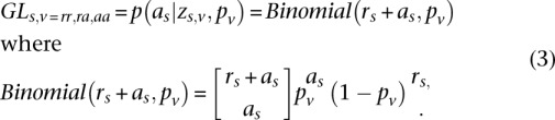
Using GLs generated by the BBMM module, we generated phased genotype imputation call sets of chromosome 20 using optimal parameters for the imputation engine (chunk size of 200 sites for 200 Markov chain Monte Carlo [MCMC] iterations) (Supplemental Material). The imputation generated highly accurate SNP genotypes when compared to OMNI microarray (Methods), with an overall discordance rate of 0.55%. This error rate is similar to the discordance rate found in site-independent, high-coverage individual calls (0.5%–1%) but is still higher than the microarray error rate (0.2%∼0.3%). In addition, the nonreference error rate, which is inclusive of all alleles that are not Ref/Ref, was 1.24% (Table 1).

Table 1.

Genotype discordance rates for SNPTools and Beagle

To evaluate genotype accuracy, we utilize benchmark genotypes generated by the 1000G with Illumina 2.5M OMNI SNP microarray. In Table 1, we compare the accuracy of data sets imputed with Beagle and SNPTools using GLs generated by SNPTools and SAMtools (Methods). Compared with SAMtools GL, SNPTools GL provided improvements in Non-Ref accuracy (Ref/Alt and Alt/Alt), with decreases in discordance from 1.40% to 1.24% and 1.67% to 1.38% when imputed using SNPTools and Beagle, respectively (Table 1). Overall, we found that SNPTools imputation was more accurate for Ref/Ref and Ref/Alt genotypes but that Beagle provided more accurate Alt/Alt imputation. A comparison of four genotype imputation methods using HapMap3 SNPs by Menelaou and Marchini (2012) also found that SNPTools provides the highest accuracy heterozygous and Non-Ref genotypes.

To evaluate haplotype quality, we utilize benchmark haplotypes generated by the 1000G for Phase 1 (Abecasis et al. 2012). These high-quality haplotypes were generated by phasing array genotypes (Illumina Omni 2.5M SNP array) for 1856 samples (all Phase 1 samples + family members + unrelated individuals for later phases of the project) using SHAPEIT (Methods; Delaneau et al. 2008, 2012). SHAPEIT handles mixtures of unrelated, duos, and trios. While SHAPEIT haplotypes are phased with statistical inference from a population and are thus not perfect, they nonetheless provide a high-quality comparison point. We compare our phasing results using SNPTools phasing with SNPTools GL against haplotypes generated by Beagle using SNPTools GL. Haplotype phasing was evaluated in the African (AFR), American (AMR), European (EUR), and Asian (ASN) populations using three metrics: switch accuracy, incorrect genotype percentage (IGP), and incorrect haplotype percentage (HIP) (Marchini et al. 2006) (Methods). In Figure 5A, we compare switch accuracy and found that switch accuracy with SNPTools was better in all populations compared with results produced by Beagle (P < 10⁻¹⁶, two-sample proportion test). When compared using IGP, SNPTools performed better in EUR and ASN populations but moderately worse than Beagle in the AMR and AFR admixture (P = 0.01, two-sample proportion test) (Fig. 5B). Evaluating HIP on all populations showed that SNPTools phased genotypes were more accurate, particularly at distances >40 kb [log₁₀ (40 kb)∼1.6] (Fig. 5C). Last, we evaluated each of the ethnic populations using SNPTools (Fig. 5C). With SNPTools (Beagle showed similar results), phasing of AFR haplotypes was less accurate at shorter distances, likely due to their higher genomic diversity, however after 100 kb [log₁₀ (100kb) = 2], all populations (EUR, AMR, and ASN) showed similar levels of HIP.

Figure 5.

Haplotype phasing accuracy evaluation. SNPTools and Beagle are compared against the benchmark haplotypes from the 1000G Phase 1. (A) Switch accuracy between SNPTools and Beagle showed that SNPTools had higher switch accuracy. (B) While SNPTools had moderately worse performance on incorrect genotype percentage (IGP) for admixture populations (American [AMR] and African [AFR]), it showed comparable performance on all other populations. (C) Incorrect haplotype percentage (HIP) for AFR samples (representative of all populations). Phasing by SNPTools and Beagle were comparable until 100 kb [log₁₀ (100kb) = 2]. At longer distances, SNPTools was moderately more accurate than Beagle. (D) Phasing by SNPTools on AFR, Asian (ASN), AMR, and European (EUR) populations shows that AFR samples were more likely to be incorrectly phased at a given distance (data not shown). However, at 100 kb, all populations have an HIP of 65%–70%.

Computational performance

SNPTools is a relatively lightweight variant calling pipeline. By using EBD, a whole genome with 4× coverage can be compressed from a 60 Gb BAM file into a 1- to 2-Gb .ebd file, a 30- to 60-fold compression. This allows for high performance input/output (I/O) when processing large numbers of samples and sites. Site discovery for the entire 1092 samples in the Phase 1 pipeline occurred in several hours. Once site discovery is complete, GL computation, using BBMM, is ∼1 h per BAM. Last, SNPTools can impute/phase ∼200,000 sites per hour when using 128 threads. As SNPTools is parallelizable, great improvements in computational time are possible (see Supplemental Material).

Discussion

Accurate variant calling (of both common and rare) from NGS data is critical for the success of many ongoing large-scale population and association studies (The 1000 Genomes Project Consortium 2010). Due to current NGS cost constraints, such consortium studies may utilize a low-coverage sequencing design (Li et al. 2011; Nielsen et al. 2011) carried out across multiple laboratories with different data generation and processing procedures. Therefore, this experimental design poses unique computational challenges for the accurate detection and genotyping of population SNPs. We herein provide an integrative pipeline, SNPTools, that applies novel algorithms to detect, impute, and phase SNPs. It has achieved high sensitivity and specificity from low-coverage, whole-genome sequencing in the 1000G data set.

We have designed our pipeline to be flexible in using inputs from other GL generation and imputation engines. For example, BBMM can intake any site list and evaluate the likelihood of potential SNPs for each sample. This means that we can utilize a comprehensive SNP list from a continually updated database such as dbSNP to ensure that every known putative SNP is evaluated in any samples in future population-based studies. Also, although we currently calculate GLs for only a single BAM, in cases where multiple BAMs are available for one sample, we can extend the above model to compute BAM-specific parameters while computing joint GLs from data observed across multiple BAMs. This is possible in the 1000G where there are BAMs from different platforms, SOLiD, Illumina, or Roche 454, for single samples using different designs (LowCov and Exome Capture). We expect this situation will become more common as exome capture is supplemented and supplanted by whole-genome sequencing. Last, our imputation engine may provide a unique pathway to incorporate prior information from SNP microarrays. For instance, known genotypes from arrays can be incorporated as strong priors (high likelihood). Given the large amount of knowledge that already and will continue to originate from array-based technology, our pipeline provides opportunities to integrate those results with NGS. Similarly our imputation platform also provides opportunities to incorporate GLs for biallelic structural variants, copy number variants, and INDELs (Lu et al. 2012) produced by other variant callers (Li et al. 2009; McKenna et al. 2010; Albers et al. 2011; DePristo et al. 2011; Handsaker et al. 2011). Nonetheless challenges remain; work on incorporating multiallelic SNPs as well as integration of polymorphic structural variants, copy number variants, and INDELs from low-coverage genomic data continues to be compelling. Adoption of these more complex genomic features will improve the fidelity of large-scale association studies.

Methods

Data set description

We applied our pipeline to LowCov Phase I BAMs (20110213 BAM index file). The data set contains 1092 individuals (1103 BAMs) from 14 populations (Americans of African ancestry in SW USA [ASW], Utah residents [CEPH] with Northern and Western European ancestry [CEU], Han Chinese in Beijing, China [CHB], Southern Han Chinese [CHB], Colombians from Medellin, Colombia [CLM], Finnish in Finland [FIN], British in England and Scotland [GBR], Iberian population in Spain [IBS], Japanese in Tokyo, Japan [JPT], Luhya in Webuye, Kenya [LWK], Mexican ancestry in Los Angeles, USA [MXL], Puerto Ricans from Puerto Rico [PUR], Toscani in Italia [TSI], and Yoruba in Ibadan, Nigeria [YRI]), representing continental groups—AFR, AMR, ASN, and EUR. These BAMs were sequenced on different platforms at nine different sequencing centers: Illumina GAII and HiSeq (946 BAMs), SOLiD (142 BAMs), and Roche 454 (15 BAMs) with an average coverage of 5× (http://www.1000genomes.org/sites/1000genomes.org/files/documents/20101214_1000genomes_samples.xls). These BAMs passed a series of consensus preprocessing procedures previously described in the Pilot paper (The 1000 Genomes Project Consortium 2010; Abecasis et al. 2012).

SNP site filtering

Although the unfiltered site list generated using our variance ratio statistic (see Results) provides high-sensitivity results, optional filtering of the site list using heuristics increases the specificity of SNP discovery, however, with some reduction in sensitivity. Our pipeline employs four widely used heuristics to improve SNP specificity: (1) maximum aggregated read depth in the population, (2) minimum aggregated read depth in the population, (3) strand bias, and (4) position bias to the read ends. For tests 1 and 2 involving population read depth, we removed SNP sites that deviated significantly from the median values for the remaining SNPs. To evaluate strand and position bias, the means of the reference and alternative bases were compared using Fisher exact test. We removed SNP sites based upon P-values (see Supplemental Material). Many of these filters can be executed on the VCF level.

SNP site validation

The 1000G Phase 1 conducted a SNP validation of 300 low-coverage sites on the VQSR2b consensus list using PCR. Two hundred ninety-seven of these sites were included in the SNPTools filtered site list. The filtered SNPTools site list was included in the 1000G Phase I release (http://www.1000genomes.org/node/506) and was combined with other call sets to produce the consensus VQSR2b (Methods) site list.

GL and genotype evaluation

SAMtools and SNPTools pipelines generated GLs at VQSR2b sites. Both sets of GL were then imputed using SNPTools and Beagle (Browning and Browning 2007). The 1000G Phase 1 VQSR2b site list is the consensus site list for the project. It was compiled with contributions from different variant callers including SNPTools.

The VQSR2b site list is located at ftp://ftp.1000genomes.ebi.ac.uk/vol1/ftp/technical/working/20110621_vqsr_sites_v2b/.

Phased imputed genotypes using SAMtools and SNPTools GL and Beagle are located at ftp://ftp.1000genomes.ebi.ac.uk/vol1/ftp/technical/working/20110512_wg_VQSRv2_GL_beagle_genotypes/. The GL are annotated directly into the vcf files for each chromosome.

Phased imputed SNPTools genotypes using SNPTools are located at ftp://ftp.1000genomes.ebi.ac.uk/vol1/ftp/release/20101123/interim_phase1_release/. GL for SAMtools were extracted from annotated VCF files from Beagle and then used for imputation in the SNPTools pipeline.

All individuals were genotyped using HumanOmni1-Quad BeadChip microarray from Illumina. Phasing was completing using SHAPEIT (Delaneau et al. 2012). The phased OMNI genotypes from the interim release are located at ftp://ftp.1000genomes.ebi.ac.uk/vol1/ftp/technical/working/20110426_omni_phased_vcfs/.

Discordance rates

We measure the error by the discordance rate (percentage) for the genotype classes, Alt/Alt, Ref/Alt, and Ref/Ref. Comparisons between discordance rates were completed using the two-sample proportion test on statistical software package R (version 2.12.0). We also evaluate a nonreference genotypes and an overall discordance rate. Total/pooled discordance rate and “non-ref” discordance rate are defined at http://www.broadinstitute.org/gsa/wiki/index.php/File:GenotypeConcordanceGenotypeErrorRate.png.

Evaluation of phased results

Phased results for chromosome 20 were compared against phased OMNI genotypes. Three different criteria were used to evaluate the accuracy of phased results (Li et al. 2011). These criteria were defined by Marchini et al. (2006) to evaluate phasing against trios.

1. Switch accuracy: Switch accuracy is one minus the percentage of switches in heterozygous sites necessary to recover the correct phase of an individual. It is defined in Lin et al. (2004) as (n – 1 – sw)/(n – 1), where n is the number of heterozygous sites and sw the number of switches between neighboring heterozygous sites needed to recover the original desired sequence (Marchini et al. 2006). Switch accuracy was calculated for each sample and averaged over the ethnic grouping.

2. IGP: This is defined as the number of heterozygotes that were phased incorrectly divided by the total number of imputed genotypes. IGP was calculated for each sample and averaged over the ethnic grouping.

3. HIP: This is the percentage of individuals whose haplotypes are not completely correct for a given distance. Note that this measurement eventually equals 100% at a long enough distance.

Data access

SNPTools can be found at http://sourceforge.net/projects/snptools/.

References

- The 1000 Genomes Project Consortium 2010. A map of human genome variation from population-scale sequencing. Nature 467: 1061–1073 [DOI] [PMC free article] [PubMed] [Google Scholar]
- Abecasis GR, Auton A, Brooks LD, DePristo MA, Durbin RM, Handsaker RE, Kang HM, Marth GT, McVean GA 2012. An integrated map of genetic variation from 1,092 human genomes. Nature 491: 56–65 [DOI] [PMC free article] [PubMed] [Google Scholar]
- Albers CA, Lunter G, Macarthur DG, McVean G, Ouwehand WH, Durbin R 2011. Dindel: Accurate indel calls from short-read data. Genome Res 21: 961–973 [DOI] [PMC free article] [PubMed] [Google Scholar]
- Bishop CM. 2006. Pattern recognition and machine learning. Springer Science, New York. [Google Scholar]
- Browning SR, Browning BL 2007. Rapid and accurate haplotype phasing and missing-data inference for whole-genome association studies by use of localized haplotype clustering. Am J Hum Genet 81: 1084–1097 [DOI] [PMC free article] [PubMed] [Google Scholar]
- Carlson CS, Eberle MA, Rieder MJ, Yi Q, Kruglyak L, Nickerson DA 2004. Selecting a maximally informative set of single-nucleotide polymorphisms for association analyses using linkage disequilibrium. Am J Hum Genet 74: 106–120. [DOI] [PMC free article] [PubMed] [Google Scholar]
- Delaneau O, Coulonges C, Zagury J-F 2008. Shape-IT: New rapid and accurate algorithm for haplotype inference. BMC Bioinformatics 9: 540. [DOI] [PMC free article] [PubMed] [Google Scholar]
- Delaneau O, Marchini J, Zagury J-F 2012. A linear complexity phasing method for thousands of genomes. Nat Methods 9: 179–181 [DOI] [PubMed] [Google Scholar]
- Dempster AP, Laird NM, Rubin DB 1977. Maximum likelihood from incomplete data via the EM algorithm. J R Stat Soc Ser B Methodol 39: 1–38 [Google Scholar]
- DePristo MA, Banks E, Poplin R, Garimella KV, Maguire JR, Hartl C, Philippakis AA, del Angel G, Rivas MA, Hanna M, et al. 2011. A framework for variation discovery and genotyping using next-generation DNA sequencing data. Nat Genet 43: 491–498 [DOI] [PMC free article] [PubMed] [Google Scholar]
- Duitama J, Kennedy J, Dinakar S, Hernández Y, Wu Y, Măndoiu II 2011. Linkage disequilibrium based genotype calling from low-coverage shotgun sequencing reads. BMC Bioinformatics 12: S53. [DOI] [PMC free article] [PubMed] [Google Scholar]
- Greenspan G, Geiger D 2004. Model-based inference of haplotype block variation. J Comput Biol 11: 493–504 [DOI] [PubMed] [Google Scholar]
- Handsaker RE, Korn JM, Nemesh J, McCarroll SA 2011. Discovery and genotyping of genome structural polymorphism by sequencing on a population scale. Nat Genet 43: 269–276 [DOI] [PMC free article] [PubMed] [Google Scholar]
- Harismendy O, Ng PC, Strausberg RL, Wang X, Stockwell TB, Beeson KY, Schork NJ, Murray SS, Topol EJ, Levy S, et al. 2009. Evaluation of next generation sequencing platforms for population targeted sequencing studies. Genome Biol 10: R32. [DOI] [PMC free article] [PubMed] [Google Scholar]
- Hodgkinson A, Eyre-Walker A 2010. Human triallelic sites: Evidence for a new mutational mechanism? Genetics 184: 233–241 [DOI] [PMC free article] [PubMed] [Google Scholar]
- Homer N, Merriman B, Nelson SF 2009. BFAST: An alignment tool for large scale genome resequencing. PLoS ONE 4: e7767. [DOI] [PMC free article] [PubMed] [Google Scholar]
- Hudson R 1983. Testing the constant-rate neutral allele model with protein sequence. Evolution 37: 203–217 [DOI] [PubMed] [Google Scholar]
- International HapMap Consortium 2005. A haplotype map of the human genome. Nature 437: 1299–1320 [DOI] [PMC free article] [PubMed] [Google Scholar]
- Kingman J 1982. Genealogy populations. J Appl Probab 19: 27–43 [Google Scholar]
- Koboldt DC, Chen K, Wylie T, Larson DE, McLellan MD, Mardis ER, Weinstock GM, Wilson RK, Ding L 2009. VarScan: Variant detection in massively parallel sequencing of individual and pooled samples. Bioinformatics 25: 2283–2285 [DOI] [PMC free article] [PubMed] [Google Scholar]
- Le SQ, Durbin R 2011. SNP detection and genotyping from low-coverage sequencing data on multiple diploid samples. Genome Res 21: 952–960 [DOI] [PMC free article] [PubMed] [Google Scholar]
- Li H 2011a. A statistical framework for SNP calling, mutation discovery, association mapping and population genetical parameter estimation from sequencing data. Bioinformatics 27: 2987–2993 [DOI] [PMC free article] [PubMed] [Google Scholar]
- Li H 2011b. Improving SNP discovery by base alignment quality. Bioinformatics 27: 1157–1158 [DOI] [PMC free article] [PubMed] [Google Scholar]
- Li H, Durbin R 2009. Fast and accurate short read alignment with Burrows-Wheeler transform. Bioinformatics 25: 1754–1760 [DOI] [PMC free article] [PubMed] [Google Scholar]
- Li N, Stephens M 2003. Modeling linkage disequilibrium and identifying recombination hotspots using single-nucleotide polymorphism data. Genetics 2233: 2213–2233 [DOI] [PMC free article] [PubMed] [Google Scholar]
- Li H, Ruan J, Durbin R 2008. Mapping short DNA sequencing reads and calling variants using mapping quality scores. Genome Res 18: 1851–1858 [DOI] [PMC free article] [PubMed] [Google Scholar]
- Li H, Handsaker B, Wysoker A, Fennell T, Ruan J, Homer N, Marth G, Abecasis G, Durbin R 2009. The sequence alignment/map format and SAMtools. Bioinformatics 25: 2078–2079 [DOI] [PMC free article] [PubMed] [Google Scholar]
- Li Y, Willer CJ, Ding J, Scheet P, Abecasis GR 2010. MaCH: Using sequence and genotype data to estimate haplotypes and unobserved genotypes. Genet Epidemiol 34: 816–834 [DOI] [PMC free article] [PubMed] [Google Scholar]
- Li Y, Sidore C, Kang HM, Boehnke M, Abecasis GR 2011. Low-coverage sequencing: Implications for design of complex trait association studies. Genome Res 21: 940–951 [DOI] [PMC free article] [PubMed] [Google Scholar]
- Lin S, Chakravarti A, Cutler DJ 2004. Haplotype and missing data inference in nuclear families. Genome Res 14: 1624–1632 [DOI] [PMC free article] [PubMed] [Google Scholar]
- Liti G, Carter DM, Moses AM, Warringer J, Parts L, James SA, Davey RP, Roberts IN, Burt A, Koufopanou V, et al. 2009. Population genomics of domestic and wild yeasts. Nature 458: 337–341 [DOI] [PMC free article] [PubMed] [Google Scholar]
- Lu JT, Wang Y, Gibbs RA, Yu F 2012. Characterizing linkage disequilibrium and evaluating imputation power of human genomic insertion-deletion polymorphisms. Genome Biol 13: R15. [DOI] [PMC free article] [PubMed] [Google Scholar]
- Marchini J, Cutler D, Patterson N, Stephens M, Eskin E, Halperin E, Lin S, Qin ZS, Munro HM, Abecasis GR, et al. 2006. A comparison of phasing algorithms for trios and unrelated individuals. Am J Hum Genet 78: 437–450 [DOI] [PMC free article] [PubMed] [Google Scholar]
- McKenna A, Hanna M, Banks E, Sivachenko A, Cibulskis K, Kernytsky A, Garimella K, Altshuler D, Gabriel S, Daly M, et al. 2010. The Genome Analysis Toolkit: A MapReduce framework for analyzing next-generation DNA sequencing data. Genome Res 20: 1297–1303 [DOI] [PMC free article] [PubMed] [Google Scholar]
- Menelaou A, Marchini J 2012. Genotype calling and phasing using next-generation sequencing reads and a haplotype scaffold. Bioinformatics 29: 1–8 [DOI] [PubMed] [Google Scholar]
- Nielsen R, Paul JS, Albrechtsen A, Song YS 2011. Genotype and SNP calling from next-generation sequencing data. Nat Rev Genet 12: 443–451 [DOI] [PMC free article] [PubMed] [Google Scholar]
- Ning Z, Cox AJ, Mullikin JC 2001. SSAHA: A fast search method for large DNA databases. Genome Res 11: 1725–1729 [DOI] [PMC free article] [PubMed] [Google Scholar]
- Scheet P, Stephens M 2006. A fast and flexible statistical model for large-scale population genotype data: Applications to inferring missing genotypes and haplotypic phase. Am J Hum Genet 78: 629–644 [DOI] [PMC free article] [PubMed] [Google Scholar]
- Shendure J, Ji H 2008. Next-generation DNA sequencing. Nat Biotechnol 26: 1135–1145 [DOI] [PubMed] [Google Scholar]
- Suzuki S, Ono N, Furusawa C, Ying B-W, Yomo T 2011. Comparison of sequence reads obtained from three next-generation sequencing platforms. PLoS ONE 6: e19534. [DOI] [PMC free article] [PubMed] [Google Scholar]