Linear mixed-effects modeling approach to FMRI group analysis

Abstract

Conventional group analysis is usually performed with Student-type t-test, regression, or standard AN(C)OVA in which the variance–covariance matrix is presumed to have a simple structure. Some correction approaches are adopted when assumptions about the covariance structure is violated. However, as experiments are designed with different degrees of sophistication, these traditional methods can become cumbersome, or even be unable to handle the situation at hand. For example, most current FMRI software packages have difficulty analyzing the following scenarios at group level: (1) taking within-subject variability into account when there are effect estimates from multiple runs or sessions; (2) continuous explanatory variables (covariates) modeling in the presence of a within-subject (repeated measures) factor, multiple subject-grouping (between-subjects) factors, or the mixture of both; (3) subject-specific adjustments in covariate modeling; (4) group analysis with estimation of hemodynamic response (HDR) function by multiple basis functions; (5) various cases of missing data in longitudinal studies; and (6) group studies involving family members or twins.

Here we present a linear mixed-effects modeling (LME) methodology that extends the conventional group analysis approach to analyze many complicated cases, including the six prototypes delineated above, whose analyses would be otherwise either difficult or unfeasible under traditional frameworks such as AN(C)OVA and general linear model (GLM). In addition, the strength of the LME framework lies in its flexibility to model and estimate the variance–covariance structures for both random effects and residuals. The intraclass correlation (ICC) values can be easily obtained with an LME model with crossed random effects, even at the presence of confounding fixed effects. The simulations of one prototypical scenario indicate that the LME modeling keeps a balance between the control for false positives and the sensitivity for activation detection. The importance of hypothesis formulation is also illustrated in the simulations. Comparisons with alternative group analysis approaches and the limitations of LME are discussed in details.

Introduction

Group analysis of FMRI datasets typically follows a two-tier approach. At the first level, the effects of interest are estimated voxel-wise in a time series regression model for each individual subject. At the second level, the effect estimates of interest are summarized and inferences generalized across subjects. The typical FMRI group analysis methodologies have matured over the past twenty years, especially using basic types of statistical tests (also known as ordinary least squares model) such as paired, one-sample, or two-sample Student t-test. With more complex designs, multi-way ANOVA models can help. Such models allow for purely categorical (qualitative, nominal, discrete, ordinal, or binary) variables that usually have two or more levels to be modeled. In addition, other traditional models such as ANCOVA and multiple regression analysis may also be adopted.

Even though it was historically developed independently from linear models or regression analysis, ANOVA can be seen as syntactic sugar for a special subgroup of linear models. Originally created by R. A. Fisher, significance testing involved in ANOVA requires cell means in a rigid and complete data structure and the decomposition of the sums of squared deviations. Of the virtues of ANOVA are the intuitive layout, technical simplicity, and computational frugality. However, this comes at the cost of design rigidity and simplistic assumptions about the variance-covariance structures. ANOVA offers limited flexibility in partitioning the variance components in the hierarchical structure of multi-levels, and corrections for the violation of assumptions such as compound symmetry,¹ and homogeneity. With both categorical and quantitative variables involved, the traditional ANCOVA framework becomes further cumbersome in handling the variance sources. These complications, plus software design flaws or users’ poor understanding, add to the difficulties and misuses of AN(C)OVA (McLaren et al., 2011) often occurring in brain imaging.

More complex experimental designs become cumbersome or impossible to handle within the traditional methods. For example, methods in most of the current FMRI software packages have difficulty handling the following scenarios at the group level: (1) taking within-subject variability into account when there are effect estimates from multiple runs or sessions; (2) continuous explanatory variables (covariates) modeling in the presence of a within-subject (repeated measures) factor, multiple subject-grouping (between-subjects) factors, or the mixture of the two; (3) subject-specific adjustments in covariate modeling; (4) group analysis with estimation of hemodynamic response (HDR) function by multiple basis functions; (5) various cases of missing data in longitudinal studies; and (6) group studies involving family members or twins.

To motivate the present exposition of the linear mixed effects approach (LME), we present a real FMRI group study to demonstrate a design complexity that requires the adoption of LME. Briefly, the experimental design involved two subject-grouping factors, age (two levels: youth and adults) and diagnosis (two levels: healthy and patients), dividing 82 subjects into four groups: 14 patient youth, 15 patient adults, 25 healthy youth, and 28 healthy adults. Stimuli were morphed images containing varying blends of two stimulus features and divided into eleven levels based on the feature blend. Stimuli were randomly presented during blocks where subjects were required to focus their attention on one of the three tasks (threat appraisal, explicit memory, and perceptual discrimination). Detailed scanning and stimulus parameters can be found in Britton et al. (under review).

The subjects were scanned in a mixed event-related and block-design experiment. Parameters for whole brain BOLD data on a 3.0 T scanner are: voxel size of 2.5×2.5×2.6 mm³, 36 contiguously interleaved slices, and repetition time (TR) of 2300 ms (TE=25 ms, FOV=240 mm, flip angle=90°). Two runs of data were acquired for each subject, and each run lasted for 11 min 8 s with 290 brain volumes. Each of the two runs included 12 randomly-ordered blocks where subjects were required to focus their attention on one of the three tasks. The tasks were randomly presented, and each was repeated four times per run. Each block randomly presented eleven distinct stimuli varying along a linear gradient of similarity, along with two blank trials to facilitate event-related analyses. The eleven stimuli represented morphed images containing varying blends of two stimulus features, ranging over 0%, 10%, …, 100%. Each stimulus lasted for 3000 ms with a 500 ms inter-stimulus interval.

At the group level, six explanatory variables considered are: 1) three subject-grouping (between-subjects) factors: age (two levels: youth and adults), diagnosis (two levels: healthy and patients), and scanner (subjects were scanned in two different scanners), 2) one within-subject (repeated-measures) factor: task with three levels, and 3) two quantitative variables: morphing levels and number of days between two phases of the experiment. Of special interest in the study are both linear and quadratic trends for the morphing effects and their interactions with the following three factors: age, diagnosis, and task. For example, does the FMRI data support the hypothesis that adolescents and adults with anxiety disorders are incapable of discriminating threat and safety cues under ambiguous situations? And what brain regions are deficit in detecting, appraising and differentiating threat? The fixed effects under consideration can be expressed as age*diagnosis*attention *morphing + age*diagnosis * attention * morphing² + scanner + days, where, in following notional convention in R (R Development Core Team, 2011), operator * for variables a and b in ‘a*b’ is interpreted as ‘a+b+a:b’, and ‘+’ and ‘:’ represent addition and interaction of all the variables including factors appearing in the term respectively.

The complexity and challenge for the analysis are five-fold: 1) the total number of variables involved, 2) the mixture of three types of variables: quantitative variables, within- and between-subjects factors, 3) the unbalanced data structure: unequal number of subjects across groups, 4) appraising and teasing apart the four-way interactions: age*diagnosis*attention*morphing, and age*diagnosis*attention*morphing², and 5) modeling the random effects: in addition to handling the potential correlation among the three tasks, the analyst should realize that each subject may deviate from the overall intercept, linear and quadratic fitting for the morphing effects. That is, we need to consider the covariance structures for the three tasks and for the three coefficients in the second-order polynomials. These intricacies are beyond the capabilities of traditional tools such as ANOVA, ANCOVA, or a general linear model (GLM, see Appendix A), but an LME framework can handle such a model.

When variance–covariance assumptions are violated, traditional ANOVA models that are special cases of LME models, can lead to inflated statistical power, as demonstrated in McLaren et al. (2011), Glaser and Friston (2007). The LME modeling strategy has recently been applied to simple cases such as the longitudinal volume changes of a brain region and cortex thickness (Bernal-Rusiel et al., 2012). The main thrust of our presentation, however, is not merely about the utility of LME under simple violations of ANOVA assumptions; rather, we introduce the LME framework as an additional tool to the brain imaging community for those cases where the traditional approach fails or does not apply at all.

The layout of the paper is as follows. First, we introduce the LME model formulation with GLM and conventional FMRI group analysis approaches as special cases. Intraclass correlation (ICC) can be defined in an LME model. Second, six prototypical examples of FMRI group analysis are outlined to showcase the uniqueness and flexibility of LME modeling strategy. Third, the implementation of LME modeling strategy in AFNI (Cox, 1996) was applied to real experimental data to overcome deficiencies with conventional GLM framework; and simulation data were used to reveal how the LME modeling performs in terms of type I error controllability and power relative to alternative approaches. Finally, we discuss its comparisons with other methodologies and the limitations of the LME approach.

Method

LME model formulation

The LME model decomposes the m_i-dimensional response or outcome vector ${\widehat{\mathbf{b}}}_i$ of the ith subject as (Pinheiro and Bates, 2000),

$${\widehat{\mathbf{b}}}_i=X_i\mathbf{a}+Z_i{\mathbf{d}}_i+{\mathbf{e}}_i,\text{or}{\widehat{\mathbf{b}}}_i\sim N\left(X_i\mathbf{a},Z_i\Psi Z_i^T+{\Sigma }_i\right),$$ (1a)

where ${\widehat{\mathbf{b}}}_{m_i\times 1}={\left({\widehat{\beta }}_1,\dots ,{\widehat{\beta }}_{m_i}\right)}^T$ are m_i effect estimates from the ith subject, a=(α₀,…,α_p)^T codes for p+1 fixed effects, d_i represents q random effects that are assumed to follow N(0, Ψ), columns of matrices X_i (of size m_i×(1+p)) and Z_i (of size m_i×q) are fixed-effects and random-effects regressors respectively, and residual term e_i is the m_i-dimensional within-subject residual vector that follows N(0, Σ_i). All the fixed effects have been incorporated in X_ia, thus the random effects d_i have a mean of 0, and the columns in Z_i are usually a subset of columns in X_i (i.e., q≤p+1). The two random effect components, d_i and e_i, are assumed independent across subjects and independent of each other for the same subject. In practice the cross-subjects variance–covariance matrix Ψ (of size q×q) can be patterned or restricted in some special form such as diagonal matrix (with q parameters), compound symmetry (with q+1 parameters), or general positive-definite symmetry (with q(q+1)/2 parameters). Similarly, for the structure of the within-subject variance-covariance matrix Σ_i (of size m_i×m_i) that shows the correlations among the within-subject residuals from the ith subject. The typical patterned structures seen in the literature for Σ_i are diagonal matrix (σ²I_mi, one parameter) associated with spherical distribution, autoregressive (AR) model (with two parameters) or autoregressive moving average (ARMA) structure, compound symmetry (with two parameters), or a general symmetric, positive semi-definite matrix (with m_i(m_i+1)/2 parameters). The response vector ${\widehat{\mathbf{b}}}_i$ in FMRI usually codes for either task/condition effects relative to the baseline or linear combinations of effects among two or more tasks/conditions.

It is noteworthy that our notation for the response or outcome variable, $\widehat{\beta }$ (or its vector form $\widehat{\mathbf{b}}$), instead of the conventional letter y (or y), reflects the following two characteristics of FMRI group analysis: 1) It is the regression coefficients (or their linear combinations) from individual subject analysis, often referred to as β values, that are taken to the group level in the conventional two-stage FMRI analysis; 2) each regression coefficient $\widehat{\beta }$ is an effect estimate (thus the hat notation ^) for BOLD response strength and is accompanied with certain reliability information.

With the subject index i hidden, the model (1a) can be further reformulated through stacking,

$$\widehat{\mathbf{b}}=X\mathbf{a}+Z\mathbf{d}+\mathbf{e}$$ (1b)

where $\widehat{\mathbf{b}}$ (of size Σm_i×1), X (of size Σm_i×(1+p)), d and e are the sequential stacking of ${\widehat{\mathbf{b}}}_i$, X_i, d_i and e_i respectively across all n subjects, and sparse matrix Z is a block-diagonal matrix with blocks of Z₁, Z₂,…, Z_n on the diagonal. That is,

$$\begin{array}{cc}\hfill \widehat{\mathbf{b}}& =\mathit{vec}\left({\widehat{\mathbf{b}}}_1,{\widehat{\mathbf{b}}}_2,\dots ,{\widehat{\mathbf{b}}}_n\right),X={\left(X_1^T,X_2^T,\dots ,X_n^T\right)}^T,\hfill \\ \hfill Z& =\text{diag}(Z_1,Z_2,\dots ,Z_n)=Z_1\oplus Z_2\oplus \dots \oplus Z_n,\mathbf{d}=\mathit{vec}({\mathbf{d}}_1,{\mathbf{d}}_2,\dots ,{\mathbf{d}}_n),\hfill \\ \hfill \mathbf{e}& =\mathit{vec}({\mathbf{e}}_1,{\mathbf{e}}_2,\dots {\mathbf{e}}_n),\hfill \end{array}$$

where vec and ⊕ are operators for column stacking and direct sum. It is typically assumed that d~N(0, ZGZ^T), and e~N(0, R), thus $\widehat{\mathbf{b}}\sim N\left(X\mathbf{a},Z\mathit{G}{Z}^T+\mathbf{R}\right)$, where G is a block-diagonal matrix with blocks of n repetitive Ψ matrices on the diagonal representing the variance-covariance structure at the group level, and R is a block-diagonal matrix with blocks of Σ₁, Σ₂, …, Σ_n on the diagonal representing the variance–covariance structure of the residuals. That is, G=diag(Ψ, Ψ, …, Ψ)=I_n⊕Ψ, and R=diag(Σ1, Σ₂, …, Σ_n), where⊕is the Kronecker product² operator. In a balanced situation where all subjects have the same amount of data (e.g., ANOVA), m₁=m₂=… m_n=m, Σ₁=Σ₂=…=Σ_n=Σ, and R=diag(Σ, Σ, …, Σ)=I_n⊕Σ. In the model formulation (1b), the random effects Zd are sometimes called “G-side” effects with “G” for grouping terms in general or group level in the context of FMRI data analysis, while e is termed as “R-side” effects with “R” for residuals.

There are several ways to characterize and differentiate the fixed- and random-effects (Gelman, 2005). A fixed effect measures the outcome at population level that is characterized by a coefficient associated to a factor level, the contrast of two factor levels, or a covariate. In contrast, a random effect indicates the deviation of each subject from the population average. To account for the observed phenomena $\widehat{\mathbf{b}}$, we may poetically say that the fixed effects Xa can be viewed as capturing the immutable and universal constants of a hypothetical population, the random effects Zd show the durable characteristics of individual subjects, and residuals e are but evanescent aberrations of the moment (Crowder and Hand, 1990). The outstanding difference between the LME model (1) and the traditional GLM (Appendix A) is that, in addition to a fixed-effects design matrix, a random-effects matrix Z is present in the LME model (1b) in which each indicator variable represents subject allocation to the levels of a random-effects component and allows one to model and then estimate the correlation structure, for example, among the multiple levels of a within-subject factor. Such explicit expression of random effects allows for multilevel and hierarchical experimental designs or data structure. Unlike GLM, LME is a nonlinear system due to the presence of multiple variance parameters, and is handled specially from both theoretical and numerical perspectives. The shrinkage phenomenon (shrinking toward zero for the random-effects estimates compared with each individual subject’s fit) in the LME system reflects a compromise between the random and fixed effects, pulling the individual fits toward the population averages (Pinheiro and Bates, 2000). Moreover, the shrinkage toward the fixed effects in the pooling process of solving LME is an indication of robustness against outlying behavior of individual subjects.

The unique feature of LME lies in its flexibility of modeling the two variance-covariance structures: Ψ and Σ_i. More specifically, when we apply the LME model (1) to group analysis of FMRI data, the vector ${\widehat{\mathbf{b}}}_i$ contains m_i effect estimates of interest or connectivity measures from the ith subject. The columns of the fixed-effects regressor matrix X_i code for categorical (e.g., positive, neutral and negative conditions in an emotion experiment, or three genotype groups – two homozygotes and one heterozygote – of subjects) and/or continuous explanatory variables (covariates). The residual term e_i measures the within-subject variability across the p+1 fixed effects, which is most often considered to have a spherical Gaussian distribution. Similarly, the columns of the random-effects matrix Z_i model the amount of deviations each subject is relative to the corresponding group effects (e.g., positive, neutral and negative condition) represented in the columns of fixed effect matrix X_i.

Conventional approaches as special cases of LME

The linear mixed-effects meta (or multilevel) analysis (MEMA) model (Appendix A) can be treated as a special scenario of the general LME model (Demidenko, 2004; Viechtbauer, 2007) in the sense that the within-subject variance estimate, ${\widehat{\sigma }}_i^2$, is available and m_i=1. In other words, when one incorporates the within-subject variability of each effect estimate into the group model, the analysis is statistically more robust (Worsley et al., 2002; Woolrich et al., 2004; Chen et al., 2012), and can be formulated under the LME scheme (1).

The traditional FMRI group analysis methods such as ANOVA, ANCOVA, multiple regression, paired, one- and two-sample Student t-tests can also be subsumed as special cases of the LME platform. For example, the LME model (1) reduces to a simple linear model with a one-sample (or paired) Student t-test with m_i=1, since each subject contributes only one effect (or contrast in the case of paired t-test) estimate, resulting in p=0, X_i=Z_i=1, d_i=0, e_i~N(0, σ²), or G=σ²I_n. The same is true for a two-sample Student t-test, except for the fixed-effects matrix X_i =(1, 0), (0, 1) or (1, 1) depending on the coding strategy and $R=\text{diag}({\sigma }_1^2{I}_{n_1},{\sigma }_2^2{I}_{n_2})$ assuming heterogeneous variances ${\sigma }_1^2$ and ${\sigma }_2^2$ between the two groups with n₁ and n₂ subjects respectively. In a balanced design with no missing cell or data, the traditional ANOVA assumes that the variance-covariance matrix Σ of the residuals e_i is of a special form such as compound symmetry (homogeneous variance and covariance across all levels of a factor), sphericity/circularity (homogeneous correlation between any two levels of a factor) and/or a stratification structure such as homo- or hetero-scedasticity in the within-subject residuals e_i involving multiple groups of subjects (Pinheiro and Bates, 2000). For example, the conventional two-way within-subject ANOVA can be reformulated under both GLM and LME (Appendix B). When covariates are considered, the conventional ANCOVA is quite easy to handle with the LME scheme, but difficult to implement under a regression framework such as GLM, especially when a within-subject variable is involved and requires the specifications of both within- and cross-subject variability.

Overall, the LME framework offers multiple advantages over the conventional AN(C)OVA scheme for its ability to handle: 1) mixture of quantitative and qualitative variables, 2) mixture of within- and between-subject variables, 3) unbalanced designs, such as unequal number of subjects or missing data, 4) no bound on the number of explanatory variables provided that enough sample size exists (e.g., at least five observations per variable), 5) multilevel (or hierarchical) variance structure, and 6) certain variance-covariance structures that violate the conventional AN(C)OVA assumptions. When economical and parsimonious assumptions such as compound symmetry or sphericity are violated, corrections such as methods proposed by Kenward and Roger (1997) inflate the estimated variances and then adjust the degrees of freedom through Satterthwaite (1946) correction. Instead of approximation, the flexibility in specifying the variance-covariance structures Ψ and Σ_i, or G and R in the LME model (1), allows one to assume alternatives such as AR and ARMA models, or a more relaxed structure such as a constant, symmetric, positive semi-definite variance-covariance matrix (the so-called “unstructured” variance-covariance matrix in the SAS terminology³) if enough data are available. For example, the residual variance–covariance matrix Σ in a traditional one-way repeated-measures (or within-subject) ANOVA is assumed to have a parsimonious structure of compound symmetry with two parameters that need to estimate (assuming k levels in the factor),

$$\Sigma ={\left(\begin{array}{cccc}\hfill {\sigma }^2\hfill & \hfill \rho {\sigma }^2\hfill & \hfill \cdots \hfill & \hfill \rho {\sigma }^2\hfill \\ \hfill \rho {\sigma }^2\hfill & \hfill {\sigma }^2\hfill & \hfill \cdots \hfill & \hfill \rho {\sigma }^2\hfill \\ \hfill ⋮\hfill & \hfill ⋮\hfill & \hfill \ddots \hfill & \hfill ⋮\hfill \\ \hfill \rho {\sigma }^2\hfill & \hfill \rho {\sigma }^2\hfill & \hfill \cdots \hfill & \hfill {\sigma }^2\hfill \end{array}\right)}_{k\times k}.$$

In contrast, when multiple samples for each factor level are available from each subject, the LME framework (1) of the corresponding model allows one to specify the residual variance–covariance structure Σ with various options such as the simplest (diagonal matrix with only one parameter), compound symmetry with two parameters, all the way up to the most general structure (general positive-definite symmetry with the most possible, k(k+1)/2, parameters),

$$\Sigma ={\left(\begin{array}{cccc}\hfill {\sigma }_1^2\hfill & \hfill {\omega }_{12}\hfill & \hfill \cdots \hfill & \hfill {\omega }_{1k}\hfill \\ \hfill {\omega }_{12}\hfill & \hfill {\sigma }_2^2\hfill & \hfill \cdots \hfill & \hfill {\omega }_{2k}\hfill \\ \hfill ⋮\hfill & \hfill ⋮\hfill & \hfill \ddots \hfill & \hfill ⋮\hfill \\ \hfill {\omega }_{1k}\hfill & \hfill {\omega }_{2k}\hfill & \hfill \cdots \hfill & \hfill {\sigma }_k^2\hfill \end{array}\right)}_{k\times k}.$$

It is noteworthy that the term Zd and e in the LME framework (1b) embody what are usually referred to as within- and between-subjects error terms under GLM and AN(C)OVA. The error partition correspondence can be seen from the LME formulation of the traditional two-way within-subject ANOVA (Appendix B). It is also this reformulation that lends it versatility in modeling both data stratifications and variance–covariance structures, and enables its applications to broader situations. With this subsumption of traditional approaches underneath the LME framework, differentiation is no longer needed in terms of the quantitative nature (categorical or continuous) of a variable and whether an explanatory variable is of interest to the researcher or not. This unified model provides us a convenient framework under which most analyses can be performed in one numerical scheme. We will show in the next section six prototypical examples where LME framework handles cases that are either cumbersome or even impossible to handle under the GLM context.

ICC formulated under LME

To investigate the test–retest reliability of FMRI data, the investigator may use the ICC to quantitatively measure the extent to which the individual levels of a grouping variable (e.g., session, scanner, site, subject) are related to each other. In other words, the ICC value reveals the consistency or reproducibility of the signal for each factor under consideration. The traditional approach to computing ICC relies on the partitioning of the total variance under the ANOVA framework (e.g., Shrout and Fleiss, 1979). For example, the popular usage of ICC(2,1) adopts a two-way random-effects single-measure ANOVA to assess the resemblance across the levels within each of the two factors (Shrout and Fleiss, 1979).

However, there are three aspects with the traditional ANOVA method in ICC assessment that could be improved: 1) explanatory variables (fixed-effects factors or covariates) are usually difficult to incorporate; 2) As in typical ANOVA, the decomposition of the total variance may lead to negative ICC values that are difficult to interpret; 3) ICC computation with a different number of variables requires a separate ANOVA model. These flaws can be avoided under the LME scheme. Suppose that one investigates three sources of variability with data acquired from different conditions, sites and subjects. In addition, age is suspected to have impact on the response. A model can be formulated with crossed random effects as follows,

$$\begin{array}{cc}\hfill & {\widehat{\beta }}_{\mathit{ijk}}={\alpha }_0+{\alpha }_1{x}_k+b_i+c_j+d_k+{\epsilon }_{\mathit{ijk}},b_i\sim N\left(0,{\tau }_1^2\right),c_j\sim N\left(0,{\tau }_2^2\right),d_k\sim N\left(0,{\tau }_3^2\right),\hfill \\ \hfill & {\epsilon }_{\mathit{ijk}}\sim N(0,{\sigma }^2),i=1,\dots ,n,j=1,\dots ,l,k=1,\dots ,m,\hfill \end{array}$$

where α₀ is an unobserved overall mean, x_k is the covariate value for the kth subject, b_i, c_j, and d_k are the unobserved random effects for the ith condition, jth site, and kth subject respectively, and ε_ijk is an unobserved residual term. The ICC values for the three sources can be defined as

$${\mathrm{ICC}}_i=\frac{{\tau }_i^2}{{\tau }_1^2+{\tau }_2^2+{\tau }_2^3+{\sigma }^2},i=1,2,3.$$

Implementation of LME modeling in AFNI

The LME framework has been implemented in a group analysis program 3dLME in AFNI in the open source statistical language R (R Core Team, 2012), taking advantage of the linear and nonlinear mixed-effects modeling packages nlme (Pinheiro et al., 2011) and lme4 (Bates et al., 2011), and parallel computing on multi-core systems with snow package (Tierney et al., 2011). Packages nlme and lme4 overlap in terms of LME modeling, but nlme exclusively has the capability to model spatial and temporal correlation structures, while lme4 can model crossed random effects and is computationally more efficient. Runtime varies from a few minutes up to many hours, depending on the data size, model complexity, and number of processors.

The fixed effects for a discrete variable (factor) in 3dLME are by default coded through dummy coding (or treatment contrast) with the first level as reference or base, although all coding strategies (Appendix C) are also available. In solving the LME system (1), the variance components are estimated through the optimization of the profiled log-restricted-likelihood of the model with a mixture of expectation-maximization (EM) and Newton algorithms. The EM algorithm starts first with 25 iterations by default, refining the initial estimates before switching to the more general Newton iterations (Pinheiro and Bates, 2000).

The conditional F-statistic for each explanatory variable is computed either sequentially (in the order the fixed effects are arranged in the model) or marginally (in the order each fixed effect enters the model as the last one).⁴ The interaction F-statistics are tested similarly. The numerators and denominators of the F-statistics are constructed similarly as in conventional ANOVA or GLM based on the random effect strata (or error partitions). In other words, the same F-statistics would be obtained in LME for the conventional ANOVA models. The degrees of freedom for the numerator and denominator of each F-statistic are also similarly determined (Pinheiro and Bates, 2000).

The fixed effect estimate and its significance for a continuous variable are straightforward because they are the direct output of modeling from the nlme package. Post hoc pairwise contrasts between two levels of a categorical variable can be obtained through direct estimation through dummy coding with a reference level, but are practically tested through package contrast (Kuhn, 2011) with conditional t-statistics. Each t-statistic tests the marginal significance of a fixed effect in the sense that all other fixed effects are included in the model already (Pinheiro and Bates, 2000).

With the capability to model crossed random effects through R package lme4 (Bates et al., 2011), we have implemented an AFNI program 3dICC that can calculate ICC values with unlimited number of variables, under the same platform of LME modeling through REML algorithms, and that renders nonnegative ICC values.

Advantageous applications of the LME framework

Prototypical example 1: group analysis with effects from multiple runs or sessions at individual subject level

FMRI data are usually acquired from each subject in multiple runs or sessions, and can be analyzed through concatenation in time series regression analysis (Chen et al., 2012), resulting in one effect estimate per condition. Alternatively, individual subject analysis can be performed with one effect estimate per condition for each run or session separately. With multiple effect estimates per condition, the common practice in FMRI data analysis is that the average effect estimate across those estimates is computed at the subject level and then fed to the group analysis. The average effect estimate per subject is typically obtained through equal weighting or fixed-effects analysis with weighting based on within-run/session variability (Chen et al., 2012; Lazar et al., 2002). The equal weighting approach makes the assumption that the cross-run/session variability is the same among all subjects, which may or may not be true, especially when the number of runs or sessions varies across subjects. A better approach is to incorporate the cross-run variability in a model under the LME scheme. In doing so, we decompose the effect estimate ${\widehat{\beta }}_{\mathit{ij}}$ from the ith subject during the jth run as

$${\widehat{\beta }}_{\mathit{ij}}={\alpha }_0+{\delta }_i+{\epsilon }_{\mathit{ij}},{\delta }_i\sim N\left(0,{\tau }^2\right),{\epsilon }_{\mathit{ij}}\sim N\left(0,{\sigma }^2\right),i=1,\dots ,n,j=1,\dots ,m_i,$$ (2)

where α₀ represents the average effect across n subjects, δ_i measures the deviation of the ith subject from the group fit α₀, ε_ij is the residual (or cross-run random effect within each subject) that indicates the deviation of effect estimate${\widehat{\beta }}_{\mathit{ij}}$ from the average effect of ith subject α₀+δ_i, and m_i is the number of runs/sessions in which the ith subject was scanned. It is reasonable to assume that the two random variables δ_i and ε_ij are independent from each other. Equivalently, the model can be written in the standard LME formulation (1a) with

$$\begin{array}{cc}\hfill {\widehat{\mathbf{b}}}_i& ={\left({\widehat{\beta }}_{i1},{\widehat{\beta }}_{i2},\dots ,{\widehat{\beta }}_{{\mathit{im}}_i}\right)}^T,\mathbf{a}={\alpha }_0,{\mathrm{X}}_i={\mathrm{Z}}_i=1_{m_i},{\mathbf{d}}_i={\delta }_i,\hfill \\ \hfill {\mathbf{e}}_i& ={\left({\epsilon }_{i1},{\epsilon }_{i2},\dots ,{\epsilon }_{{\mathit{im}}_i}\right)}^T,i=1,\dots ,n.\hfill \end{array}$$

With the assumptions of Ψ=τ², and Σ_i = σ²I_mi in the model (1a), or G=τ²I_n and $\mathit{R}={\sigma }^2{I}_M(M={\sum }_{i=1}^n{m}_i)$ in the model (1b), the LME framework has the flexibility of handling varying sample size m_i across subjects and the capability of weighting among subjects in estimating the within-subject variability σ² (cf. σ² is assumed the same across subjects in the conventional group analysis).

Even if the number of runs or sessions remains the same across subjects, it would be advantageous to bring the effect estimates from individual runs or sessions to group level, especially when the data structure is complex. For example, with effect estimates averaged across runs or sessions, a conventional one-way within-subject ANOVA can be represented under the GLM notation,

$${\widehat{\beta }}_{\mathit{ij}}=\mu +{\alpha }_j+b_i+{\epsilon }_{\mathit{ij}},b_i\sim N\left(0,{\tau }^2\right),{\epsilon }_{\mathit{ij}}\sim N\left(0,{\sigma }^2\right),i=1,\dots ,n,j=1,\dots ,m,$$ (3a)

where ${\widehat{\beta }}_{\mathit{ij}}$ is the effect estimate at the jth level of factor A for the ith subject, μ is the grand mean free of any factor effect, α_j is the jth level effect of factor A, b_i is the deviation of the ith subject, and ε_ij represents the residual associated with the ith subject at the jth level of factor A. Due to the fact that no data duplication exists, the conventional ANOVA with sphericity assumption, although economical, is the only choice at voxel level.

However, if one takes the effect estimates from individual runs or sessions to group analysis, the model (3a) changes to

$$\begin{array}{cc}\hfill {\widehat{\beta }}_{\mathit{ijk}}& =\mu +{\alpha }_j+b_i+c_{\mathit{ij}}+{\epsilon }_{\mathit{ijk}},b_i\sim N\left(0,{\tau }_1^2\right),c_{\mathit{ij}}\sim N\left(0,{\tau }_2^2\right),\hfill \\ \hfill {\epsilon }_{\mathit{ijk}}& \sim N\left(0,{\sigma }^2\right),i=1,\dots ,n,j=1,\dots ,m,k=1,\dots ,l,\hfill \end{array}$$ (3b)

where k is the run or session index, and c_ij, absent in the model (3a), models the deviation of the ith subject’s effect at the jth level of factor A. As shown in the model formulation (3b), the across-run variability is accounted for under LME. Furthermore, instead of assuming compound symmetry, one could further extend the model (3b), and account for unequal correlations (and unequal variances) across the factor levels with a general positive definite symmetric variance–covariance structure. However, such a covariance structure with the model (3b) cannot be modeled under the conventional ANOVA or GLM framework, but becomes straightforward as an LME instance. For simplicity, the model (3b) is presented with a balanced data structure; however, LME modeling allows for unequal number of runs as well as missing data (e.g., some subjects may not have effect estimates for all levels, cf. prototypical example 5).

Prototypical example 2: subject-specific random effect in covariate modeling

Trend detection across conditions, runs, or sessions is of special interest because of the implied effect of modulation, habituation, or saturation. Such trend analysis can be performed at individual level through, for example, effect comparisons, weighted test across multiple effects, or amplitude (or parametric) modulation. Furthermore, it would be usually desirable to generalize the trend effect through group analysis. A prototypical example is an FMRI experiment of n subjects with m stimuli along a linear gradient of similarity. Suppose that we want to test whether the BOLD response estimate ${\widehat{\beta }}_{\mathit{ij}}$ of relevant regions in the brain of the ith subject can be fitted, for example, in a quadratic fashion with respect to the jth image degradation x_j=(j–1)×10% (j=1, …, m) with the following model,

$${\widehat{\beta }}_{\mathit{ij}}={\alpha }_0+{\alpha }_1{x}_j+{\alpha }_2{x}_j^2+{\delta }_{0i}+{\delta }_{1i}{x}_j+{\delta }_{2i}{x}_j^2+{\epsilon }_{\mathit{ij}},i=1,\dots ,n,j=1,\dots ,m,$$

where ε_ij is the residual (within-subject error), and the random effects of the intercept (δ_0i), slope (δ_1i) and curvature (δ_2i) in the model allow each subject to have a separate second-order polynomial fitting from the group average intercept (α₀), linearity (α₁) and curvature (α₂). In other words, with these three random components the effect estimate from individual level, ${\widehat{\beta }}_{\mathit{ij}}$, is fitted with a subject-specific intercept (α₀+δ_0i), slope (α₁+δ_1i) and curvature (α₂+δ_2i). The model can be repackaged as the LME model (1) with

$$\begin{array}{cc}\hfill {\widehat{\mathbf{b}}}_i& =\left(\begin{array}{c}\hfill {\widehat{\beta }}_{i1}\hfill \\ \hfill {\widehat{\beta }}_{i2}\hfill \\ \hfill ⋮\hfill \\ \hfill {\widehat{\beta }}_{\mathit{im}}\hfill \end{array}\right),\mathbf{a}=\left(\begin{array}{c}\hfill {\alpha }_0\hfill \\ \hfill {\alpha }_1\hfill \\ \hfill {\alpha }_2\hfill \end{array}\right),{\mathrm{X}}_i={\mathrm{Z}}_i=\left(\begin{array}{ccc}\hfill 1\hfill & \hfill x_1\hfill & \hfill x_1^2\hfill \\ \hfill 1\hfill & \hfill x_2\hfill & \hfill x_2^2\hfill \\ \hfill ⋮\hfill & \hfill ⋮\hfill & \hfill ⋮\hfill \\ \hfill 1\hfill & \hfill x_m\hfill & \hfill x_m^2\hfill \end{array}\right),\hfill \\ \hfill {\mathbf{d}}_i& =\left(\begin{array}{c}\hfill {\delta }_{0i}\hfill \\ \hfill {\delta }_{1i}\hfill \\ \hfill {\delta }_{2i}\hfill \end{array}\right),{\mathbf{e}}_i=\left(\begin{array}{c}\hfill {\epsilon }_{i1}\hfill \\ \hfill {\epsilon }_{i2}\hfill \\ \hfill ⋮\hfill \\ \hfill {\epsilon }_{\mathit{im}}\hfill \end{array}\right),\hfill \\ \hfill {\mathbf{d}}_i& \sim N(0,{\Psi }_{3\times 3}),{\mathbf{e}}_i\sim N\left(0,{\sigma }^2{I}_{m\times m}\right),i=1,\dots ,n.\hfill \end{array}$$

In the model format (1b), G=I_n ⊕Ψ_3×3, and R=σI_nm×nm. By default the intercept α₀ is the average group effect at no degradation, but the group average effect at any other specific degradation can be inferred through properly centering the degradation variable x_j. The parameters to be estimated are fixed effects a, cross-subject variability Ψ, and within-subject variability σ². In this case the three random effect components (intercept δ_0i, slope δ_1i and curvature δ_2i) are more reasonably modeled with Ψ being a symmetric, positive semi-definite variance–covariance matrix (with six unknown parameters) than some special structures such as compound symmetry (same variance and covariance across the conditions). In other words, it is difficult to à priori justify that the variance–covariance matrix for the random effects of intercept, slope, and curvature has some preset structure. If the analysis is performed at one specific voxel or a region of interest, one could assess and compare models with various variance–covariance structures through likelihood ratio test and the comparisons of Akaike information criterion (AIC) or Bayesian information criterion (BIC) (Pinheiro and Bates, 2000). However, when running simultaneous voxel-wise analysis for all the voxels in the brain, such model tuning process is impractical from two reasons: a) the computation cost is generally great; b) the optimal model may end up different across voxels or regions in the brain.

Alternatively, the linearity (α₁) and curvature (α₂) for each subject could be obtained at individual level, and then the group effects are estimated separately with, for example, Student t-test. However, such an approach is suboptimal and not as robust to individual outlying data as the LME method. This is a feature of the shrinkage phenomenon of LME: the estimated slope (α₁+δ_1i) and curvature (α₂+δ_2i) for each subject with LME tend to be pulled toward the group effects (α₁ and α₂), compared with the estimates obtained from individual subject analysis.

Prototypical example 3: covariate modeling in the presence of a within-subject factor

Suppose that a study recruits subjects for scanning under m different conditions (e.g., m=3 emotions: positive, neutral, and negative), and the model would be one-way repeated-measures ANOVA at group level. We further assume that amplitude (or parametric) modulation is performed with reaction time (RT) collected at trial level in individual subject analysis to account for cross-trial variability. However, the average RT may vary across the m conditions and across all subjects as well. The incorporation of the average RT at the condition level of each subject in group analysis may further account for both within- and cross-subject variability, improving the statistical power. Two aspects of effect testing could be of typical research interest: a) whether the correlation between RT and BOLD response differs across the conditions; b) whether any difference exists among the condition after accounting for RT effect and for both within- and across-subject variability in RT. Although beyond the scope of the traditional ANCOVA framework that handles only between-subjects, not within-subject, factors, it is relatively easy to analyze the situation under the LME scheme. In this case we partition the effect estimate of the jth condition effect from ith subject, ${\widehat{\beta }}_{\mathit{ij}}$, as

$${\widehat{\beta }}_{\mathit{ij}}={\alpha }_{0j}+{\alpha }_{1j}{x}_{\mathit{ij}}+{\delta }_{0i}+{\delta }_{1i}{x}_{\mathit{ij}}+{\epsilon }_{\mathit{ij}},i=1,\dots ,n,j=1,\dots ,m,$$

where x_ij is the ith subject’s average RT under the jth condition, α_0j represents the group effect of the jth condition corresponding to reaction time x=0, α_1j is the marginal effect of RT under the jth condition at group level, δ1iX_ij measures the deviation of the linear fit of ith subject from the group fit α_1jX_ij, and ε_ij is the residual term (within-subject error) that reflects the deviation of ${\widehat{\beta }}_{\mathit{ij}}$ from the linear fit of ith subject. The above system allows a separate linear fit per condition for the RT data, and the ith subject’s fit varies from the linearity with a random slope δ_1i. The model can be reformatted as under the LME formulation (1a) with

$$\begin{array}{cc}\hfill {\widehat{\mathbf{b}}}_i& =\left(\begin{array}{c}\hfill {\widehat{\beta }}_{i1}\hfill \\ \hfill {\widehat{\beta }}_{i2}\hfill \\ \hfill ⋮\hfill \\ \hfill {\widehat{\beta }}_{\mathit{im}}\hfill \end{array}\right),X_i={\left(\begin{array}{ccccccc}\hfill 1\hfill & \hfill x_{i1}\hfill & \hfill 0\hfill & \hfill 0\hfill & \hfill \cdots \hfill & \hfill 0\hfill & \hfill 0\hfill \\ \hfill 0\hfill & \hfill 0\hfill & \hfill 1\hfill & \hfill x_{i2}\hfill & \hfill \cdots \hfill & \hfill 0\hfill & \hfill 0\hfill \\ \hfill ⋮\hfill & \hfill ⋮\hfill & \hfill ⋮\hfill & \hfill ⋮\hfill & \hfill \cdots \hfill & \hfill ⋮\hfill & \hfill ⋮\hfill \\ \hfill 0\hfill & \hfill 0\hfill & \hfill 0\hfill & \hfill 0\hfill & \hfill \cdots \hfill & \hfill 1\hfill & \hfill x_{\mathit{im}}\hfill \end{array}\right)}_{m\times 2m},\hfill \\ \hfill {\mathrm{Z}}_i& ={\left(\begin{array}{cc}\hfill 1\hfill & \hfill x_{i1}\hfill \\ \hfill 1\hfill & \hfill x_{i2}\hfill \\ \hfill ⋮\hfill & \hfill ⋮\hfill \\ \hfill 1\hfill & \hfill x_{\mathit{im}}\hfill \end{array}\right)}_{m\times 2},\mathbf{a}={\left(\begin{array}{c}\hfill {\alpha }_{01}\hfill \\ \hfill {\alpha }_{11}\hfill \\ \hfill {\alpha }_{02}\hfill \\ \hfill {\alpha }_{12}\hfill \\ \hfill ⋮\hfill \\ \hfill {\alpha }_{0m}\hfill \\ \hfill {\alpha }_{1m}\hfill \end{array}\right)}_{2m\times 1},{\mathbf{d}}_i=\left(\begin{array}{c}\hfill {\delta }_{0i}\hfill \\ \hfill {\delta }_{1i}\hfill \end{array}\right),{\mathbf{e}}_i=\left(\begin{array}{c}\hfill {\epsilon }_{i1}\hfill \\ \hfill {\epsilon }_{i2}\hfill \\ \hfill ⋮\hfill \\ \hfill {\epsilon }_{\mathit{im}}\hfill \end{array}\right),\hfill \\ \hfill {\mathbf{d}}_i& \sim N(0,{\Psi }_{2\times 2}),{\mathbf{e}}_i\sim N\left(0,{\sigma }^2{I}_m\right),i=1,2,\dots ,n.\hfill \end{array}$$

In the model (1b) formulation, G=I_n⊕Ψ_2×2, and R=σ²I_mn. Without loss of generality the model can be expanded from linear to a higher order polynomial fit. On the other hand, the model can be simplified if no interaction exists between the conditions and RT (dropping index j in α_1j) or when the covariate is measured at the subject level (e.g., age, IQ, etc.) (dropping index j in α_1j and X_ij),

$${\widehat{\beta }}_{\mathit{ij}}={\alpha }_{0j}+{\alpha }_1{x}_i+{\delta }_{0i}+{\delta }_{1i}{x}_{\mathit{ij}}+{\epsilon }_{\mathit{ij}},i=1,\dots ,n,j=1,\dots ,m.$$

Prototypical example 4: hemodynamic response modeled with multiple basis functions

The hemodynamic response (HDR) is commonly presumed to have a relatively fixed shape in modeling (Cohen, 1997; Henson et al., 2002), which works reasonably well especially with block designs, thanks to the physiological effect of temporal blurring modeled through convolution between stimulus timing and the assumed HDR function. However, it is not always realistic to believe that the HDR shape does not vary significantly across subjects, brain regions, tasks/conditions, and trials (Aguirre et al., 1998; Handwerker et al., 2004). One way to capture such shape variability is through the use of multiple basis functions (e.g., deconvolution or finite impulse response (FIR) modeling) in the time series regression analysis (Henson and Friston, 2007; Saad et al., 2006), which results in several consecutive effect estimates at individual subject level, showing the progression of the HDR corresponding to each condition/task.

At group level the shape differences are sometimes ignored by relying on a summarized effect size such as the area under the curve (AUC) (Beauchamp et al., 2003) or the coefficient of the principal basis function (e.g., Gamma variate) with other coefficients (e.g., time and dispersion derivatives) being à priori assumed to contain little information. With the AUC approach, the consecutive effects are summed over time to produce one value per condition, and then one adopts the same group analysis strategy as the HDR modeling with a fixed shape. However, the AUC approach can mask important information about HDR shape (e.g., HDR might have delayed peak, slower upstroke, different signs or durations), nullifying the original goal of modeling the HDR shape. Indeed, there have been instances where HDR shape differences are the target of interest at group level (Alvarez et al., 2011; Geier et al., 2007; Weissman et al., 2006).

In taking the m individual values of the reassembled HDR function, ${\widehat{\beta }}_{i1},\dots ,{\widehat{\beta }}_{\mathit{im}}$, to group analysis, we set a zero intercept in the LME model (1a) with X_i=I_m, Z_i=1, d_i~N(0, τ²), and e_i~N(0, Σ); that is,

$${\widehat{\beta }}_{\mathit{ij}}={\alpha }_j{x}_{\mathit{ij}}+{\delta }_i+{\epsilon }_{\mathit{ij}},i=1,\dots ,n,j=1,\dots ,m.$$

In addition, we use cell mean coding (Appendix C) for the convenience of interpretation,

$$x_{\mathit{ij}}=\{\begin{array}{cc}\hfill 1,\hfill & \hfill i\text{th sybject is at}j\text{th level}\\ \hfill 0,\hfill & \hfill \text{otherwise}.\end{array}\phantom{\}}$$

The coefficient α_j in the model conveniently shows the HDR effect for the jth time grid. Under the model formulation (1b), G=τ² I_n and R=diag(Σ, Σ, …, Σ)=I_n⊕Σ. Unlike the previous prototypes, it makes more sense to assume a serially correlated variance-covariance structure in the within-subject residuals e_i such as AR(1) or ARMA(1,1) (with two and three parameters respectively). One can make inference about the null hypothesis,

$$H_0:{\alpha }_1=\dots ={\alpha }_m=0\left(\text{no HDR at any time point}\right).$$ (4a)

When H₀ is rejected with an F-test, the HDR is significant among at least one of the m locations. This null hypothesis is similar to the one for omnibus F-test in a regression model or global null hypothesis involved in appropriate conjunction analysis (Nichols et al., 2005). It is not rare to see in the literature that the significance testing at group level with multiple basis functions is typically performed with the following null hypothesis in the context of one- or higher-way repeated-measures (or within-subject) ANOVA,

$$H_0:{\alpha }_1=\dots ={\alpha }_m.$$ (4b)

However, the F-test associated with (4b) is inappropriate in the context, leading to questionable inferences: if (4b) is rejected, it corresponds to the main effect of the m levels, and indicates that the magnitude of HDR is significantly different across those m locations. Instead (4a) should be considered in this scenario (Alvarez et al., 2011). In addition, when more than one group is involved, group comparisons can be analyzed; analysis with a within-subject factor and covariate modeling are also possible.

To reiterate, the subtle difference between the two null hypotheses (4a) and (4b) is the following: The rejection of (4a) occurs when any of the coefficients is significantly different from 0, which would suggest a consistent response at least at one time point over the duration modeled. This type of test is what is typically sought. The rejection of (4b) indicates that at least one coefficient differed from the others, which indicates that the response was not constant at some point over the duration modeled. The subtle differences will be highlighted in the section Simulations comparing LME with traditional approaches in Applications and results.

Prototypical example 5: Missing data in longitudinal study

There are two different types of missing data in FMRI group analysis. The first one involves missing effect estimates at voxel level from individual subjects that often occur in FMRI data along the edge of the brain, due to factors such as data acquisition limitations, susceptibility artifacts, and imperfect alignment in spatial normalization to standard space. The issue is even more prevalent in electrocorticographical (ECoG) data in neurosurgical patients where not all patients get the same cortical coverage and the subdural electrodes (SDEs) are implanted on cortex only in the immediate vicinity (Conner et al., 2011). This type of missing data issue can be handled at voxel level (Chen et al., 2012) or through multiple imputation (Vaden et al., 2012).

The second type of missing data is at the whole brain level. In a typical longitudinal study each subject is observed repeatedly over long periods of time, or before and after some treatment (exercise, drug intake, surgery, etc.). Participant dropout is a prevalent phenomenon in such studies, which complicates the statistical analysis due to the broken balance of the data structure. Even in an experiment involving multiple tasks, some subjects may fail to perform one of the tasks, and such subjects are usually removed from the conventional group analysis with ANOVA or paired t-test due to the loss of balance in data structure.

The essential issue about the second type of missing data in LME modeling is whether they can be considered as missing at random (MAR) or missing completely at random (MCAR). If the data is systemically missing (e.g., all female subjects did not perform task #3) including covariate-dependent dropout (CDD) and non-ignorable missingness (NI), subsequent analysis with LME would lead to biased inferences. Handling such a scenario requires alternate daunting computations and various imputation methods (e.g., Allison, 2001; Little and Rubin, 2002; Schafer, 1997) that are not currently applied in the neuroimaging community. However when the situation is truly MCAR/MAR, LME overcomes the difficulty of the conventional ANOVA or GLM where missing data breaks the rigid variance-covariance structure of the model. In ANOVA or GLM, the effect estimates and their standard errors are based on observed and expected mean sum of squares (or partitioned error strata), and the integrity in data balance is essential in partitioning the error terms. With enough subjects and observation per variable (e.g., 10-30), MCAR/MAR would not lead to information loss (Keselman et al., 2001; Little and Rubin, 2002). Parameters in the LME model are estimated through optimizing the (restricted) maximum likelihood function where a balanced structure is not required. In other words, the LME models are fitted using REML and produce results that are optimal with relatively accurate and robust results in significance testing (Pinheiro and Bates, 2000). Nevertheless, a simple and robust approach to a MCAR/MAR situation is to abandon those subjects with the missing data, or to adopt a simple method such as a Student t-test, when enough number of subjects remains.

For example, suppose that 20 children participated in an experiment that included two fear conditions each of which was arranged in two separate sessions. For various reasons (e.g., data quality, head motion issues, failure to show up, etc.) 13 subjects had usable data for both conditions, two and five subjects had data only for conditions 1 and 2 respectively. With the traditional group analysis approach of paired t-test to comparing the two conditions, only the data from those 13 subjects can be used, while the seven subjects that contain only one of the two conditions could also be included under the LME modeling framework.

Prototypical example 6: Data analysis in family or twin studies

Due to genetic information flow and inheritance, data collected among family members can be considerably correlated. FMRI data analyses of family members, including siblings and especially monozygotic (MZ) or dizygotic (DZ) twins, are increasingly common (Stoffers et al., 2012). To properly account for the heritability among the subjects, special handling has to be employed in the model. Here we present two cases to demonstrate the LME flexibility in analyzing data that involve family members. In the first, one focuses on the fixed effects while in the other random effects are of research interest.

In the first case let us assume that the effect estimate from the jth member in the ith family, ${\widehat{\beta }}_{\mathit{ij}}$, can be partitioned into

$${\widehat{\beta }}_{\mathit{ij}}={\alpha }_0+{\alpha }_1{x}_{\mathit{ij}}+{\delta }_{0i}+{\delta }_{1i}{x}_{\mathit{ij}}+{\epsilon }_{\mathit{ij}},i=1,\dots ,n,j=1,\dots ,m,$$

where α₀ is the overall mean across all families, x_ij is a fixed-effects variable (e.g., behavioral measure, control versus patients, or genotype coding), α₁ indicates the covariate effect, δ_0i and δ_1ix_ij embody the deviation of the linear fit of the ith family from the overall fit, and ε_ij codes for the within-subject residual term. Although one explanatory variable (besides the intercept) is considered in the model above, the number of fixed-effects can be increased without loss of generality. Compared to the previous prototypes, one unique feature about this model is that the data structure hinges around families instead of individual subjects.

This model can be reformatted as under the LME formulation (1a) in a similar way to Prototype 3 (covariate modeling in the presence of a within-subject factor),

$$\begin{array}{cc}\hfill {\widehat{\mathbf{b}}}_i& =\left(\begin{array}{c}\hfill {\widehat{\beta }}_{i1}\hfill \\ \hfill {\widehat{\beta }}_{i2}\hfill \\ \hfill ⋮\hfill \\ \hfill {\widehat{\beta }}_{\mathit{im}}\hfill \end{array}\right),X_i={\mathrm{Z}}_i=\left(\begin{array}{cc}\hfill 1\hfill & \hfill x_{i1}\hfill \\ \hfill 1\hfill & \hfill x_{i2}\hfill \\ \hfill ⋮\hfill & \hfill ⋮\hfill \\ \hfill 1\hfill & \hfill x_{\mathit{im}}\hfill \end{array}\right),\mathbf{a}=\left(\begin{array}{c}\hfill {\alpha }_0\hfill \\ \hfill {\alpha }_1\hfill \end{array}\right),\hfill \\ \hfill {\mathbf{d}}_i& =\left(\begin{array}{c}\hfill {\delta }_{0i}\hfill \\ \hfill {\delta }_{1i}\hfill \end{array}\right),{\mathbf{e}}_i=\left(\begin{array}{c}\hfill {\epsilon }_{i1}\hfill \\ \hfill {\epsilon }_{i2}\hfill \\ \hfill ⋮\hfill \\ \hfill {\epsilon }_{\mathit{im}}\hfill \end{array}\right),\hfill \\ \hfill {\mathbf{d}}_i& \sim N(0,{\Psi }_{2\times 2}),{\mathbf{e}}_i\sim N(0,{\Sigma }_{m\times m}),i=1,2,\dots ,n.\hfill \end{array}$$

In the model (1b) formulation, G=I_n ⊗ Ψ_2×2, and R=diag(∑, ∑, …,∑)=I_n⊗∑. As the covariances (off-diagonal terms of ∑) in phenotypic effects across the m family members are usually partitioned into additive genetic, dominance genetic, common environmental, and unique environmental effects (Neale et al., 1989), the correlation (or kinship) is different between parents, between a parent and a son/daughter, between siblings, and between DZ/MZ twins. In this example, the correlations for additive genetic effect are 1, 0.5 and 0.5 between MZ twins, between DZ twins, and between parent and son/daughter respectively, while the correlations for dominance genetic effect is 1, 0.25, and 0 respectively (Falconer and MacKay, 1996). Similar to the concept of kinship matrix in the mixed-effects modeling of association mapping (Yu et al., 2006), a generic symmetric, positive semi-definite variance-covariance matrix for both Ψ_2×2 and ∑_m×m is likely more reasonable than the presumption of compound symmetry for whole-brain analysis.

When missing data occur or when families have unequal number of members, the within-family variance–covariance is structured as R=diag(∑₁, ∑₂, …, ∑_n), and the LME framework should work well if the situation can be considered as MAR. If only DZ twins are involved in the study, the variance-covariance structure ∑ can be simplified to ${\sigma }^2{I}_2$, and, with the assumption ${\Psi }_{2\times 2}=\left(\begin{array}{cc}\hfill {\tau }_0^2\hfill & \hfill {\tau }_{01}^2\hfill \\ \hfill {\tau }_{01}^2\hfill & \hfill {\tau }_1^2\hfill \end{array}\right)$, the correlation between a DZ twin pair in the ith family is thus modeled as $\frac{{\tau }_0^2+{\tau }_{01}^2{\sum }_{j=1}^2{x}_{\mathit{ij}}+{\tau }_1^2{\prod }_{j=1}^2{x}_{\mathit{ij}}}{{\prod }_{j=1}^2\sqrt[]{{\tau }_0^2+2x_{\mathit{ij}}{\tau }_{01}^2+{\tau }_1^2{x}_{\mathit{ij}}^2+{\sigma }^2}}$. The approach has effectively been applied to a twins study with resting-state network analysis (Stoffers et al., 2012).

In the second scenario the identification of variance sources is of research interest. Suppose that m effect estimates (BOLD response, DTI data, or structural images) are collected from twin pairs who are either MZ or DZ. The kth measure (k=1, 2, …, m) from the jth twin (j=1, 2) of the ith pair (i=1, 2, …, n) can be fitted with an LME model (Min et al., 2012),

$$\begin{array}{cc}\hfill {\widehat{\beta }}_{\mathit{ijk}}=& \text{fixed}\text{effects}+p_{\mathit{ij}}+z_{i\left(j\right)}+e_{\mathit{ij}}\hfill \\ \hfill & +{\epsilon }_{\mathit{ijk}},p_{\mathit{ij}}\sim N\left(0,{\tau }_p^2\right),z_{i\left(j\right)}\sim N\left(0,{\tau }_z^2\right),e_{\mathit{ij}}\sim N\left(0,{\tau }_e^2\right),\hfill \\ \hfill {\epsilon }_{\mathit{ijk}}\sim N& \left(0,{\sigma }^2\right),i=1,2,j=1,2,k=1,\dots ,m,\hfill \end{array}$$

where the random effects p_ij, z_i(j), e_ij, and ε_ijj are pair (shared by a twin pair, regardless of zygosity), zygosity (common to an MZ pair but not by a DZ pair), individual environment, and residual effects, respectively. The variance partition is different from but related to the popular ACE or ADE model (Nicholson et al., 2011).

Under the above LME model, the familiality (the familial proportion of biological variance) can be obtained as $\frac{{\tau }_p^2+{\tau }_z^2}{{\tau }_p^2+{\tau }_z^2+{\tau }_e^2+{\sigma }^2},$ where ${\tau }_p^2$ indicates the combined phenotypic variance of genetic and common environmental effects between a DZ pair regardless of zygosity. While DZ pairs are common to half of the additive variance and their common environmental variance, the MZ pairs have an additional component, the other half of the additive variance, which is modeled by ${\tau }_z^2$. Therefore the heritability can be estimated as $\frac{2{\tau }_z^2}{{\tau }_p^2+{\tau }_z^2+{\tau }_e^2+{\sigma }^2}$ (Min et al., 2012). It is noteworthy that both familiality and heritability are essentially two ICC measures as discussed in section ICC formulated under LME. A recent development (Wang et al., 2011) recommended a likelihood ratio test with a mixture of χ²-distribution for the significance of familiality and heritability.

Applications and results

LME with real data

The following two candidate models were initially adopted to fit the data presented in Introduction,

$${\widehat{\beta }}_{i\left(\mathit{jk}\right)\mathit{lm}}=\text{fixed}\text{effects}+{\delta }_{0i,l}+{\delta }_{0i}+{\epsilon }_{i\left(\mathit{jk}\right)\mathit{lm}},$$ (5a)

$${\widehat{\beta }}_{i\left(\mathit{jk}\right)\mathit{lm}}=\text{fixed}\text{effects}+{\delta }_{0i,l}+{\delta }_{0i}+{\delta }_{1i}{x}_m+{\delta }_{2i}{x}_m^2+{\epsilon }_{i\left(\mathit{jk}\right)\mathit{lm}}.$$ (5b)

The “fixed effects” in the model included age*diagnosis* attention*morphing+age*diagnosis*attention * morphing²+scanner+days, where, following notional convention in R, operator * for variables a and b in ‘a*b’ is interpreted as ‘a+b+a:b’, and ‘+’ and ‘:’ are addition and interaction of all the variables and factors appearing in the term. The indices i, j, k, l and m code for subject, age, diagnosis, attention and morphing respectively (i=1, 2, …, 82; j=1, 2; k=1, 2; l=1, 2, 3; and m=1, 2, …, 11). The notation i(jk) implies each subject is nested within the two subject-grouping factors, age (j) and diagnosis (k). The difference between the two models (5a) and (5b) is that each subject has a unique intercept (or baseline) in the former while the latter allows variability for intercept, linear and quadratic fitting across subjects. To improve interpretability and reduce the amount of collinearity in the model, both quantitative variables (morphing x_m and number of days) were centered on their respective mean, and the second order orthogonal Legendre polynomials were used to fit for the morphing effect.

The random effects in the above two models (5a) and (5b) can be formulated respectively under the LME scheme (1a) with

$$Z_i=\left(\begin{array}{cccc}\hfill 1\hfill & \hfill 0\hfill & \hfill 0\hfill & \hfill 1\hfill \\ \hfill 0\hfill & \hfill 1\hfill & \hfill 0\hfill & \hfill 1\hfill \\ \hfill 0\hfill & \hfill 0\hfill & \hfill 1\hfill & \hfill 1\hfill \end{array}\right)\oplus 1_{11},{\mathbf{d}}_i=\left(\begin{array}{c}\hfill {\delta }_{0i,1}\hfill \\ \hfill {\delta }_{0i,2}\hfill \\ \hfill {\delta }_{0i,3}\hfill \\ \hfill {\delta }_{0i}\hfill \end{array}\right),\Psi =\left(\begin{array}{cc}\hfill {\Psi }_{3\times 3}^{\left(1\right)}\hfill & \hfill 0_{3\times 1}\hfill \\ \hfill 0_{1\times 3}\hfill & \hfill {\Psi }_{1\times 1}^{\left(2\right)}\hfill \end{array}\right),$$ (6a)

$$Z_i=\left(\begin{array}{cccccc}\hfill 1\hfill & \hfill 0\hfill & \hfill 0\hfill & \hfill 1\hfill & \hfill 1\hfill & \hfill 1\hfill \\ \hfill 0\hfill & \hfill 1\hfill & \hfill 0\hfill & \hfill 1\hfill & \hfill 1\hfill & \hfill 1\hfill \\ \hfill 0\hfill & \hfill 0\hfill & \hfill 1\hfill & \hfill 1\hfill & \hfill 1\hfill & \hfill 1\hfill \end{array}\right)\oplus 1_{11},{\mathbf{d}}_i=\left(\begin{array}{c}\hfill {\delta }_{0i,1}\hfill \\ \hfill {\delta }_{0i,2}\hfill \\ \hfill {\delta }_{0i,3}\hfill \\ \hfill {\delta }_{0i}\hfill \\ \hfill {\delta }_{1i}\hfill \\ \hfill {\delta }_{2i}\hfill \end{array}\right),\Psi =\left(\begin{array}{cc}\hfill {\Psi }_{3\times 3}^{\left(1\right)}\hfill & \hfill 0_{3\times 3}\hfill \\ \hfill 0_{3\times 3}\hfill & \hfill {\Psi }_{3\times 3}^{\left(2\right)}\hfill \end{array}\right),$$ (6b)

where i=1, 2, …, 82. Furthermore, δ_0i,1, δ_0i,2, and δ_0i,3 are random effects for the three attention levels with a variance–covariance structure ${\Psi }_{3\times 3}^{\left(1\right)}$, and δ_0i, δ_1i, and δ_2i code for random intercept, slope and curvature of the ith subject with a variance–covariance structure ${\Psi }_{1\times 1}^{\left(2\right)}$ or ${\Psi }_{3\times 3}^{\left(2\right)}$.

Although not practical for whole brain analysis due to high computation cost and heterogeneity across voxels, model building can be performed at a specific voxel or region. To demonstrate the building process and the LME flexibility, we fitted the two models (5a) and (5b) with the data from a voxel at the subgenual anterior cingulate (−9, 26, −9), with each model further split into different variance–covariance structures for random effects (G) and residuals (R) (Table 1). Models with different random effects can be compared through either the lesser of the information criteria or likelihood ratio test with chi-square distribution (with the degrees of freedom being the difference in the number of parameters used in the models) (Pinheiro and Bates, 2000). The results indicate that the model (5a) with random-effect specification (6a) struck a better balance with the experiment data at this voxel; specifically the variance–covariance matrix ${\Psi }_{3\times 3}^{\left(1\right)}$ for the three attentions was assumed to have a symmetric, positive definite structure with G=I₈₂⊗Ψ, while ∑=σ² I₃₃ (fitting A in Table 1).

Table 1.

Comparisons among models at a voxel in sgACC with different variance–covariance structures for random effects and residuals.

Model	Formulation		(6a)		(6b)
	Fitting		A	B	C	D
Ψ	Attention Ψ1)	structure	pdSymm	pdCompSymm	pdSymm	pdSymm
		parameters	6	2	6	6
	Morph Ψ2)	structure	intercept	intercept	pdSymm	pdCompSymm
		parameters	1	1	6	2
DF			46	42	51	47
AIC			1431.455	1444.031	1440.332	1433.455
BIC			1624.398	1620.196	1654.246	1630.592
logLik			−669.7277	−680.0156	−669.1657	−669.7277
LR (relative to model A), p			-	20.57585, 0.0004	1.124, 0.95	0, 1

¹⁾Coding: Specifications for variance–covariance structure used in nlme package: pdSymm– general positive-definite symmetry; pdCompSymm – compound symmetry; intercept – random effect for intercept only (without linear and quadratic random effects)

²⁾DF – degrees of freedom; AIC – Aikaike Information Criterion; BIC – Bayesian Information Criterion; logLik – log restricted maximum likelihood; LR: likelihood ratio test with χ²(k) comparing two models (where k is the DF difference between the two models), and p – probability corresponding to the χ²(k) value.

At the whole brain level the model (5a) with random-effect specification (6a) was fitted with the experiment data. The variance–covariance matrix ${\Psi }_{3\times 3}^{\left(1\right)}$ was assumed to have a symmetric, positive definite structure with G=I₈₂⊗Ψ, while ∑=σ²I₃₃ (fitting A in Table 1). The analysis, unfeasible under the GLM framework, was performed with 3dLME with 2706 effect estimates (regression coefficients) from individual subject analysis (82 subjects×3 attentions×11 morphs/subject).

Two regions, subgenual anterior cingulate and ventromedial prefrontal cortex were identified to have four-way interaction age×diagnosis×attention×morphing² (Fig. 1 and Table 2). The localization of these two regions was further used to guide ROI analysis and show consistency with behavioral data results.

Fig. 1.

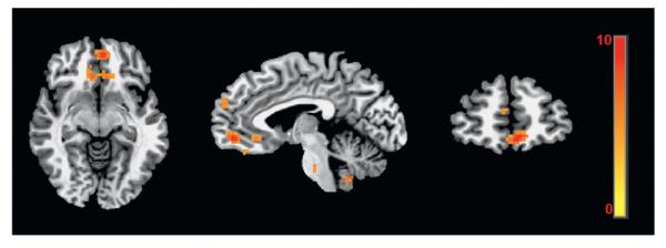
Four-way interactions (diagnosis×age group×cognitive instruction×quadratic trend) were detected with LMEmodeling in two regions, the subgenual anterior cingulate (−9, 26,−9) and the ventromedial prefrontal cortex (4, 49, −6). Image displayed in radiological convention (left=right) with colors indicating the F (2, 2592)-statistic range with FWE corrected p=0.05.

Table 2.

Tests for all the main effects and their interactions at a voxel in sgACC.

Term	F-value	Significance
Age	0.125 (1, 76)	0.724
Diagnosis	1.577 (1, 76)	0.213
Attention	3.962 (2, 2592)	0.019
Morph	0.278 (1, 2592)	0.598
Morph2	0.604 (1, 2592)	0.437
Age: diagnosis	0.032 (1, 76)	0.859
Age: attention	3.005 (2, 2592)	0.050
Age: morph	0.009 (1, 2592)	0.924
Age: morph2	7.488 (1, 2592)	6.25e–3
Diagnosis: attention	0.501 (2, 2592)	0.606
Diagnosis: morph	0.144 (1, 2592)	0.704
Diagnosis: morph2	5.578 (1, 2592)	0.018
Attention: morph	0.687 (2, 2592)	0.503
Attention: morph2	4.610 (2, 2592)	0.010
Age: diagnosis:attention	0.419 (2, 2592)	0.658
Age: diagnosis: morph	0.041 (1, 2592)	0.840
Age: diagnosis: morph2	13.079 (1, 2592)	3.04e–4
Age: attention: morph	1.159 (2, 2592)	0.314
Age: attention: morph2	6.478 (2, 2592)	1.56e–3
Diagnosis: attention: morph	0.100 (2, 2592)	0.905
Diagnosis: attention: morph2	4.261 (2, 2592)	0.014
Age: diagnosis: attention: morph	0.444 (2, 2592)	0.642
Age: diagnosis: attention: morph2	8.285(2, 2592)	2.59e–4
Scanner	0.272 (1, 76)	0.604
Days	0.684 (1, 76)	0.411

The two numbers within parentheses in the F-value column are the numerator and denominator degrees of freedom respectively

Simulations comparing LME with traditional approaches

Simulated data were generated using prototypical example 4 (serially correlated HDR results) so that the LME approach could be directly compared to the conventional ANOVA method. The simulations were designed to assess power and controllability for type I errors from the following three perspectives: a) the amount of serial correlation in the residuals of HDR estimates, b) the violation of assumption about the residuals (two levels: AR(1) and sphericity), and c) null hypothesis (two levels: proper and improper hypothesis (4a) and (4b)). The two factors in b) and c) form a 2×2 factorial design, leading to four analysis approaches with the aim to examine the performance of the conventional approaches when their underlying assumptions are violated or when an improper null hypothesis is tested:

1. LME+AR(1)+N0: LME with AR(1) assumption of the residuals testing the hypothesis (4a),

2. LME+AR(1)+N1: LME with AR(1) assumption of the residuals testing the hypothesis (4b),

3. LME+AR(0)+N0: LME with white noise assumption testing the hypothesis (4a), and

4. LME+AR(0)+N1: the conventional ANOVA with sphericity assumption testing the hypothesis (4b).

Here N0 and N1 indicate that the null hypotheses correspond to the LME models without and with an intercept respectively. The approach of LME+AR(0)+N1 can also be framed under the GLM formulation.

Three sample sizes (number of subjects) were considered: n=10,15, and 20. The simulated data were in the units of percent signal change. Nine effect estimates were created with a Gamma variate function (Cohen, 1997) peaked at an amplitude of 1, simulating an HDR spanning 16 s with TR=2 s. Additional AR(1) noise with variance of 1 was added to the nine effect estimates of each subject at one of the ten equally-spaced serial correlations: 0.0, 0.1, …, 0.9. With 5,000 datasets generated, type I error rate and power were assessed through counting the datasets with the perspective F-statistic surpassing the threshold corresponding to the nominal significance level of 0.05.

The simulation results are summarized with plots in Fig. 2 for n=15 subjects. In general, LME+AR(1)+N0 achieves the best balanced compromise between type I errors and power than the other three methods. More specifically, it demonstrates the overall controllability in false positives across the whole range of serial correlations. When no serial correlation exists in the noise, all four methods have reasonable control for false positives; however, the improper hypothesis (4b) leads to underpowered inferences. When serial correlation exists in the noise, the AR(1) modeling largely provides proper control for the false positives, and the slightly liberal type I error rate may be due to the fact that the variance estimates have to be nonnegative while the sum of squares for some terms in the conventional ANOVA is allowed to become negative so that individual sums of squares can add up to the total. In contrast, the type I errors in the two methods with AR not modeled are not properly controlled when the serial correlation in the residuals goes beyond 0.2. For all four methods, the power mostly deteriorates as the serial correlation in the residuals increases. When the AR(1) parameter is below 0.6, the improper hypothesis (4b) largely under-powers the significance testing, while the temporal correlation, if not modeled, significantly inflates the power. LME+AR(0)+N0 achieves the highest power (at the cost of poor type I error control), ANOVA is the worst, and the other two are in between. When serial correlation is present in the noise, methods without AR modeling inflate the statistical power at the cost of poor type I error control. As the AR(1) parameter goes above 0.6, methods with serial correlation modeled overtake the other two without AR modeling in power performance. Nevertheless, LME+AR(1)+N0 outperforms the conventional ANOVA in power achievement across the whole correlation spectrum. The above assessments and trends are roughly the same with the simulations of n=10 and 20 subjects. These simulation results highlight the importance of forming a proper hypothesis, and demonstrate the impact of assumption violation: poor controllability for type I errors and inflated power.

Fig. 2.

Simulation results for type I error and power with 15 subjects. Nine effect estimates from each subject were created to simulate the HDR over 16 s and contained AR(1) residuals with serial correlation at 10 equally-spaced values (0, 0.1, ..., 0.9). Four analysis approaches were considered with 2 (with serial correlation modeled and without)×2 (proper and improper hypothesis) factorial layout. The curves were fitted through loess smoothing with the second order of local polynomials

Discussion

The conventional statistical analysis that is still popular in general statistical education emphasizes the dichotomy of categorical and quantitative (or continuous) variables, while the differentiation of fixed versus random effects is usually minimally discussed. In addition, the balance of data structure (without missing data) is usually a prerequisite for the traditional approaches such as paired t-test, ANOVA structure and GLM approach when within-subject factors are involved.

The LME modeling scheme provides a different perspective in the sense that the boundary between categorical and quantitative variables is blurred and the full integrity of data structure is not needed. Instead, the emphasis is placed on the fixed/random effects dichotomy, the hierarchical structure of random effects, and the model building process in which the modeler engages the analysis interactively with the data. It is this paradigm shift that engenders the modeling flexibility that cannot be reached under the conventional framework. When few regions are to be tested, (i.e. ROI-based analysis), unlike the decomposition of the sums of squared deviations under the rigid framework of the conventional approach, the LME scheme offers model selection by fine-tuning the variance–covariance structure at both cross- and within-unit (subject, family) levels, while counterbalancing between model complexity and fit through likelihood ratio test (e.g., Table 1).

Modeling flexibility of LME platform

The LME approach provides a platform that describes a relationship between a response variable (e.g., BOLD response) and some explanatory variables that have been observed along with (e.g., face vs. house stimuli), or are believed to have impact upon (e.g., males vs. females), the response variable. Under the LME scheme, the response variable is usually collected from multiple observational units (e.g., subjects or families), and the fixed effects are considered coming from the reproducible components of the explanatory variables such as the levels of a factor or the effect of a quantitative variable. In contrast, random effects represent the deviations of the samples (e.g., subjects) from the fixed effects.

All the conventional approaches such as t-tests, linear models, and AN(C)OVA can be subsumed into the LME framework. While more complex to set up and less computationally efficient, the LME methodology shines with the following advantages: 1) the flexibility of allowing both categorical and quantitative variables, 2) modeling the correlation structures of those random effects, 3) the capability in handling scenarios such complex designs, crossed random-effects variables, and absence of data balance, as demonstrated in the six prototypical examples, and 4) the capability to accommodate nonlinear dynamics (e.g., psychophysics, behavioral measures) using systems such as asymptotic, bi-exponential, logistic, or Michaelis–Menten relationship.

Importance of model specifications

The importance of model specifications can be demonstrated with prototypical example 1 in which the effect estimate ${\widehat{\beta }}_{\mathit{ij}}$ of the ith subject during the jth run is modeled with the LME formulation (2). For comparison, we drop the deviation δ_i of the ith subject’s effect from the group mean α₀, and replace (2) with a fixed-effects model,

$${\widehat{\beta }}_{\mathit{ij}}={\alpha }_0+{\epsilon }_{\mathit{ij}},{\epsilon }_{\mathit{ij}}\sim N\left(0,{\sigma }^2\right),i=1,\dots ,n,j=1,\dots ,m_i.$$ (2a)

The fixed-effect model (2a) can be treated as a special case of the LME model (2) in which the random effects are constrained by δ_i=0, i=1, …, n. It may sound surprising and puzzling to note that the fixed-effect model (2a) renders a smaller standard error for the group mean α₀, leading to a higher t-statistic value than the LME model (2). The pivotal difference is that each subject is allowed to have a unique average effect α₀+δ_i in the LME model (2). In other words, the overall effect α₀ in the LME model (2) is simply estimated not as one common within-subject effect as in the fixed-effect model (2a), but the average of the varying (or random) effects across all subjects. A natural (and maybe seemingly counterintuitive) question is, why does a better (or more precise) model not lead to a more precise or reliable estimate for the effect of interest? The answer lies in the underlying assumption of the fixed-effect model (2a): the m_i effect estimates, ${\widehat{\beta }}_{\mathit{ij}}$ (j=1, …, m_i) of the ith subject from all the m_i runs are mistakenly assumed to be independent although they are not independent. Such an inappropriate assumption leads to the underestimation of the reliability (or standard error) of the overall effect estimate.

A model with broader flexibility gives more room for data variability and correlation stratifications. As an appropriate model characterizes the uncertainty of effect estimate more accurately than its alternatives, the flexibility may have to pay at the cost of effect estimate with a lower, not higher, precision. The moral of the above counterintuitive phenomenon is that modeling should not be plainly considered as a process that hinges on the statistical power, but focuses more on an appropriate model with adequate assumptions. Under inappropriate assumptions, a statistical analysis may inflate the statistical power as previously demonstrated in McLaren et al. (2011) even under relatively simple scenarios. Some publications in neuroimaging adopted the model (2a) with effect estimates directly from multiple runs or sessions, leading to highly inflated significance (McLaren et al., 2011). Although not optimal as the LME model (2), using the average effect estimates across runs or sessions from each subject would at least avoid this inflation problem.

Different approaches to modeling fixed and random effects

The selection of explanatory variables in GLM is as much an art as modeling in general. If one empirically believes that specific variables can mostly account for the data variability, a model can be à priori applied without any building process. This is largely the case in FMRI individual analysis where task-related effects, slow drift, and head motion are typically plugged into the model even though some effects (e.g., head motion) are not necessarily always present. On the other hand, when such prior information is lacking or uncertainty exists, the selection of explanatory variables may be limited by the number of data points or degrees of freedom available, and the risk of over-fitting may occur. Various techniques can assist the investigator in the model building process. For example, data examination through visualization or plotting can and should play a more crucial role in data preprocessing and modeling than what is practiced in reality. Stepwise methods (forward selection and backward elimination) are sometimes employed although they may be controversial. These considerations apply to the covariate selection at group level as well. One could consider infinite covariates in group analysis, for instance, age, psychometric measures, sex, genotype, education level, brain volume, cortical thickness, Big Five personality traits, cultural, ethnic, and socioeconomic attributes, etc. However, the typical number of subjects for group analysis does not allow one to have the luxury to exhaust the possible modeling strategies.

The same considerations apply to modeling random effects as well. If prior information is available (e.g., serial correlation in HDR estimates), one may adopt a parsimonious model with relatively meager parameters. When only one effect estimate per condition or task is available, the investigator is limited to a rigid covariance structure such as compound symmetry assumption in a voxel-wise model involving a within-subject factor, as shown in the conventional ANOVAs. If prior information about correlation structure is lacking, one can resort to the data and adopt a less constrained model for random effects (cf. the six prototypical examples). When multiple effect estimates per condition (e.g., from multiple runs) are available, one would have bigger wiggle room in parameterizing the covariance structures. The counterbalance between the two extreme approaches can be achieved and measured through criteria such as AIC and BIC, or likelihood ratio tests that are typically employed in model comparisons.

Comparisons of LME with other approaches to FMRI group analysis

In the conventional GLM (see Appendix A) an explanatory variable can be a subject-grouping factor, but not a within-subject (or repeated-measures) factor in which all the levels could be correlated to some extent. Such limitation can be overcome (Rutherford, 2001) to include within-subject factors by considering subject as a variable in the model through, for example, effect coding (see Appendix C). However, the coding process for subjects and their interactions with fixed-effect factors becomes relatively tedious, especially when more than one categorical factor is involved. Furthermore, the error terms have to be properly separated for effect testing when more than one factor is involved; otherwise inflated significance may occur (McLaren et al., 2011). These are the reasons that only one within-subject or one-way between-subject AN(C)OVA is usually considered with this approach in FMRI group analysis, as shown in SPM and FSL implementations.

The traditional suite of group analysis programs (3dttest++, 3dMEMA, 3dANOVAx, and GroupAna) in AFNI can analyze data structure with t-tests, ANCOVA with between-subjects factors, up to four-way ANOVA. A recent new program 3dMVM (http://afni.nimh.nih.gov/sscc/gangc/MVM.html) has been developed with multivariate GLM approach that can handle the conventional AN(C)OVA without bound on the number of explanatory variables provided that the sample size is appropriate (e.g., at least five observations per variable). In addition, it allows unequal number of subjects across groups.

As another recent extension of the GLM approach to FMRI group analysis, a Matlab package called GLM Flex (http://nmr.mgh.harvard.edu/harvardagingbrain/People/AaronSchultz/GLM_Flex.html) takes up to six-way interactions. More importantly, the error terms are properly partitioned across factors using the covariance estimates pooled across voxels. Covariate modeling is also possible with GLM Flex, but not allowed in the presence of a within-subject variable (i.e., repeated-measures ANCOVA), which requires the LME approach as shown in prototypical example 3. Under slightly different assumptions, GLM Flex and 3dMVM can handle cases 1 and 4 of the six prototypical examples.

Another recent development (Skup et al., 2012) uses multi-scale adaptive regression model (MARM) and its variants that address two major issues: potential problems involving spatial smoothing and voxelwise versus spatial modeling. The approach was developed specifically to deal with structural data such as T1 images or DTI data where the traditional method with volume data may suffer from poor alignment, and this point is highlighted by its major applications with the real data examples. Nevertheless, the methodology could be applied to group analysis of functional FMRI data; for example, twin studies (e.g., prototypical example 6) may benefit from the adoption of MARM (Li et al., 2012). It remains to be seen how MARM compares to the LME framework in terms of application breadth and modeling flexibility.

Limitations of LME

The LME flexibility to modeling data with complex structure comes with the difficulty in assigning the degrees of freedom for each testing statistic. The number of degrees of freedom is the dimension of the subspace under the null hypothesis when the data are projected on the linearly spanned space of the model matrix. With a balanced data structure with simple covariance layout and no missing data, the degrees of freedom can be clearly defined, and the F-statistics are truly F-distributed under the Gaussian assumption, as shown in the traditional ANOVA computations. However, with sophisticated covariance structure, missing data, or crossed random effects, the LME framework is not really a linear system in the sense that the presence of multiple variance parameters allows only for asymptotic approximations. The asymptotic property leads to not only the occasional failure of numerical convergence, but also the challenges in deciding the degrees of freedom; that is, the F-values are asymptotic as well.

Currently the degrees of freedom in 3dLME are based on the inner/outer property of each term relative to the random factor (e.g., subject) adopted in the R package nlme (Pinheiro and Bates, 2000). However, such an assignment approach for the degrees of freedom is controversial for a few scenarios. For example, when two or more within-subject factors are involved or when data structure is not balanced, the assignment tends to be inaccurate. Parametric bootstrapping (Halekoh and Højsgaard, in press) and Markov chain Monte Carlo (MCMC) simulations sampling (Baayen, 2011; Bates et al., 2011; Skaug et al., 2012) have been available for a more accurate significance testing, but they are not practical for FMRI group analysis due to the very high computational cost. A promising approach with the Kenward–Roger adjustment is currently under development (Halekoh and Højsgaard, in press) that may hold promise in improving the accuracy of significance testing for 3dLME in the future. As a rule of thumb, a higher number of subjects (e.g., 20 or more) would provide more robust analysis with 3dLME.

Conclusions

LME is a flexible modeling approach that handles complex experimental designs that Student t-test, AN(C)OVA frameworks cannot. LME can model a variety of variance–covariance structures, covariate modeling with multiple factors including either within-subject (or repeated-measures) or between-subjects (subject-grouping or independent-measures) factors, or both.

The six prototypical FMRI group analysis scenarios were presented to exemplify the unique advantages of the LME approach. ICC values can also be computed under the LME paradigm that can account for confounding effects. Our simulations indicate that the LME modeling strategy, when applied to FMRI group analysis, shows reasonable control for false positives and achieves sizeable statistical power.

Appendix A. General linear model (GLM)

The concept of general linear model provides a broad platform that subsumes Student t-test, F-test, ANOVA, ordinary linear regression, ANCOVA, MANOCA, and MANCOA. A GLM framework for FMRI group analysis can be formulated for the conventional group analysis of p+1 fixed effects with FMRI data of n subjects,

$${\widehat{\beta }}_i=\sum _{j=0}^p{\alpha }_i{\mathbf{x}}_{\mathit{ij}}+{\delta }_i={\mathbf{x}}_i^T\mathbf{a}+{\delta }_i,\text{or}{\widehat{\beta }}_i\sim N\left({\mathbf{x}}_i^T,\mathbf{a},{\tau }^2\right),i=1,2,..,n,$$ (7a)

where response variable ${\widehat{\beta }}_i$ is the effect estimate from the individual analysis of the ith subject, $x_i^T=(x_{i0},\dots ,x_{\mathit{ip}})$ denotes the intercept (x_i0=1) and p explanatory variables, a=(α₀,…,α_p)^T contains the p+1 fixed effect or regression coefficients, and δ_i is the subject-specific random component that is assumed to follow N(0, τ²). We can rewrite the GLM in a concise matrix formulation,

$$\widehat{\mathbf{b}}=X^T\mathbf{a}+\mathbf{d},\text{or}\widehat{\mathbf{b}}\sim N\left(X^T,\mathbf{a},{\tau }^2{I}_n\right),$$ (7b)

where ${\widehat{\mathbf{b}}}_{n\times 1}={\left({\widehat{\beta }}_1,\dots ,{\widehat{\beta }}_n\right)}^T,X_{n\times (p+1)}={({\mathbf{x}}_1,\dots ,{\mathbf{x}}_n)}^T,{\mathbf{d}}_{n\times 1}={({\delta }_1,\dots ,{\delta }_n)}^T\sim N\left(0,{\tau }^2{I}_n\right)$, and I_n is an n×n identity matrix. A one-sample Student t-test corresponds to model (7) with p=0. If p≥1, x_ij can be an indicator (dummy) variable coding, for example, the group to which the ith subject belongs, or a continuous variable, or an interaction among fixed effects. If τ² is significantly different from 0, the presence of d in (7b) may indicate either a heterogeneous group of subjects, or heterogeneity due to some unknown or unobservable factors. The former possibility may necessitate considering some subject-specific modulators. Furthermore, the effect estimate ${\widehat{\beta }}_i$ typically replaces the corresponding “true” effect β_i in “summary statistics” approach (Penny and Holmes, 2007) with the sampling error or estimate precision of ${\widehat{\beta }}_i$ ignored in the fixed-effects regression model (7). Most group analysis approaches can be formulated under the GLM framework (7), such as one-sample and paired t-tests, analyses with two ormore groups (e.g., two-sample t-test), and with continuous explanatory variables (e.g., age, IQ, etc.).

A statistically more robust model than (7) would be one that incorporates the within-subject variability, such as linear mixed-effect meta analysis (MEMA) (Worsley et al., 2002; Woolrich et al., 2004; Chen et al., 2012). More specifically, when the precision information (or variance) of the effect estimate ${\widehat{\beta }}_i$ is incorporated in the GLM (7), we have a mixed-effect multilevel system,

$${\widehat{\beta }}_i=\sum _{j=0}^p{\alpha }_i{x}_{\mathit{ij}}+{\delta }_i+{\epsilon }_i={\mathbf{x}}_i^T\mathbf{a}+{\delta }_i+{\epsilon }_i,\text{or}{\widehat{\beta }}_i\sim N\left({\mathbf{x}}_i^T\mathbf{a},{\tau }^2+{\sigma }_i^2\right),i=1,2,..,n,$$ (8a)

or,

$$\widehat{\mathbf{b}}=X^T\mathbf{a}+\mathbf{d}+\mathbf{e},\text{or}\widehat{\mathbf{b}}\sim N\left(X^T\mathbf{a},{\tau }^2,I_n+\Phi \right),$$ (8b)

where ${\mathbf{e}}_{n\times 1}={({\epsilon }_1,\dots ,{\epsilon }_n)}^T,{\Phi }_{n\times n}=\text{diag}{\left({\widehat{\sigma }}_1^2,\dots ,{\widehat{\sigma }}_n^2\right)}^T$, and ${\widehat{\sigma }}_i^2$ is the estimated variance for ${\sigma }_i^2$ from the individual analysis of the ith subject with the assumption ${\epsilon }_i\sim N(0,{\sigma }_i^2)$ (Chen et al., 2012).

The principal difference between the GLM(7) and MEMA (8) is that the latter model explicitly includes estimated within-subject variability (instead of presuming equal reliability across subjects), renderingmore accurate estimate and significance testing of group effect. However, a difficulty with such a robust approach with the MEMA model (8) occurs in handling the correlation structure among the multiple levels of a within-subject (or repeated-measures) factor.

Appendix B. LME formulation of two-way within-subject ANOVA

The conventional two-way within-subject (or repeated-measures) ANOVA can be formulated with a cell mean model under the GLM framework,

$$\begin{array}{cc}\hfill {\widehat{\beta }}_{\mathit{ijk}}=& {\alpha }^{\left(0\right)}+{\alpha }_j^{\left(A\right)}+{\alpha }_k^{\left(B\right)}+{\alpha }_{\mathit{jk}}^{\left(\mathit{AB}\right)}+b_i+r_{\mathit{ij}}+c_{\mathit{ik}}\hfill \\ \hfill & +{\epsilon }_{\mathit{ijk}},b_i\sim N\left(0,{\tau }_1^2\right),r_{\mathit{ij}}\sim N\left(0,{\tau }_2^2\right),c_{\mathit{ik}}\sim N\left(0,{\tau }_3^2\right),\hfill \\ \hfill {\epsilon }_{\mathit{ijk}}\sim N& \left(0,{\sigma }^2\right),i=1,\dots ,n,j=1,\dots ,l,k=1,\dots ,m,\hfill \end{array}$$ (9)

where ${\widehat{\beta }}_{\mathit{ijk}}$ is the effect estimate at the jth level of factor A and the kth level of factor B for the ith subject, μ is the grand mean free of any factor effect, ${\alpha }_j^{\left(A\right)}$ is the jth level effect of factor A, ${\alpha }_k^{\left(B\right)}$ is the kth level effect of factor B, ${\alpha }_{\mathit{jk}}^{\left(\mathit{AB}\right)}$ is the interaction effect at the jth level of factor A and the kth level of factor B, b_i is the deviation of the ith subject, r_ij is the interaction effect between the ith subject and the jth level of factor A, c_ik is the interaction effect between the ith subject and the kth level of factor B, and ε_ijk represents the residual associated with the ith subject at the jth level of factor A and the kth level of factor B.

The above GLM setup (9) for two-way within-subject ANOVA can be treated as an LME model of crossed random effects with exactly the same formulation (Pinheiro and Bates, 2000) with μ, α_j, β_k and γ_jk representing the fixed effects and b_i, r_ij and c_ik coding the random effects. And the formulation (9) can also be reformulated as (1a) with the following notations,⁵

$$\begin{array}{cc}\hfill {\widehat{\mathbf{b}}}_i& ={\left({\widehat{\beta }}_{i11,}\dots ,{\widehat{\beta }}_{i1l,}\dots ,{\widehat{\beta }}_{\mathit{im}1,}\dots ,{\widehat{\beta }}_{\mathit{iml}}\right)}^T,\hfill \\ \hfill \mathbf{a}& ={\left({\alpha }^{\left(0\right)},{\alpha }_1^{\left(A\right)},\dots ,{\alpha }_l^{\left(A\right)},{\alpha }_1^{\left(B\right)},\dots ,{\alpha }_m^{\left(B\right)},{\alpha }_{11}^{\left(\mathit{AB}\right)},\dots ,{\alpha }_{1l}^{\left(\mathit{AB}\right)},\dots ,{\alpha }_{m1}^{\left(\mathit{AB}\right)},\dots ,{\alpha }_{\mathit{ml}}^{\left(\mathit{AB}\right)}\right)}^T,\hfill \\ \hfill {\mathrm{X}}_i& =(1_{\mathit{lm}},I_m\otimes 1_l,1_l\otimes I_m,I_{\mathit{lm}}),{\mathrm{Z}}_i=(1_{\mathit{lm}},I_m\otimes 1_l,1_l\otimes I_m),\hfill \\ \hfill {\mathbf{d}}_i& ={\left(b_i,r_{i1},\dots ,r_{\mathit{il}},c_{i1},\dots c_{\mathit{im}}\right)}^T,{\mathbf{e}}_i={({\epsilon }_{i11},\dots ,{\epsilon }_{i1l,}\dots ,{\epsilon }_{\mathit{im}1,}\dots ,{\epsilon }_{\mathit{iml}})}^T,i=1,\dots ,n.\hfill \end{array}$$

where I_k is an identity matrix of size k, and 1_k denotes for a column vector of ones with its subscript k indicating the length. If a block diagonal variance–covariance structure is assumed for the random effects d_i, $\mathrm{Var}\left({\mathbf{d}}_i\right)={({\tau }_1^2,{\tau }_2^2,{\tau }_3^2)}^T\otimes \text{diag}(1,I_l,I_m)$, the LME model is essentially equivalent to the traditional two-way within-subject ANOVA with a compound symmetry structure for the random effects. However, the LME platform allows more room for flexibility in modeling the randomeffects. For example, the strict assumption of compound symmetry for Var(d_i) can be relaxed if justified. In addition, the rigid ANOVA data structure is not required under LME; that is, missing cells are allowed (e.g., no data is available from one subject at the level j₀ of factor A and level k₀ of factor B). Alternatively, the LME model for two-way within-subject ANOVA can be reduced to a random intercept model (without random terms r_ij and c_ik, for example) when necessary.

Appendix C. Coding a discrete variable

Both the fixed- and random-effect matrices X_i and Z_i in the LME model (3) involve quantifying categorical variables as indicators through various coding schemes, and deserve a brief description here. These indicator variables represent subject allocations to the k levels of a categorical variable (or factor). Although theoretically there are infinite approaches to coding or parameterizing a categorical variable x, three popular coding methods are typically seen in the literature due to their convenient interpretability.

A) Dummy coding (or treatment contrast). This scheme takes 0 and 1 values to allocate subjects among the k levels of a factor. Due to the presence of default intercept or constant in the model, only (k-1) indicators are considered to avoid multicollinearity and assigned by 1s, and one level is chosen to serve as a reference or base level and coded with

$$x_{\mathit{ij}}=\{\begin{array}{cc}\hfill 1,\hfill & \hfill i\text{th subject at}j\text{th level},\text{and}j\ne k\\ \hfill 0,\hfill & \hfill \text{otherwise}\end{array}\phantom{\}}$$ (10a)

implies that the corresponding effect shows the difference between the jth level (j=1, 2, …, k) and the reference (e.g., kth) level. The fixed-effect matrix X_i (of size k×k) for ith subject is of the structure (assuming the absence of other within-subject factors), in which each row corresponds to a level of the factor and the first column is associated with the intercept while the other (k-1) columns represent the (k-1) indicator variables,

$$X_i={\left(\begin{array}{ccccc}\hfill 1\hfill & \hfill 1\hfill & \hfill 0\hfill & \hfill \cdots \hfill & \hfill 0\hfill \\ \hfill 1\hfill & \hfill 0\hfill & \hfill 1\hfill & \hfill \cdots \hfill & \hfill 0\hfill \\ \hfill ⋮\hfill & \hfill ⋮\hfill & \hfill ⋮\hfill & \hfill \ddots \hfill & \hfill ⋮\hfill \\ \hfill 1\hfill & \hfill 0\hfill & \hfill 0\hfill & \hfill \cdots \hfill & \hfill 1\hfill \\ \hfill 1\hfill & \hfill 0\hfill & \hfill 0\hfill & \hfill \cdots \hfill & \hfill 0\hfill \end{array}\right)}_{k\times k}.$$

B) Effect (or deviation) coding. Instead of setting one level of the factor as reference or base that is denoted by all indicator variables taking value 0, the indicator variables in effect or deviation coding take the value −1 for the reference level. With the kth level as a reference, the coefficient associated with

$$x_{\mathit{ij}}=\{\begin{array}{cc}\hfill 1,\hfill & \hfill i\text{th subject at}j\text{th level},\text{and}j\ne k\\ \hfill 0,\hfill & \hfill i\text{th subject not at}j\text{th level},\text{and}j\ne k\\ \hfill -1,\hfill & \hfill i\text{th subject at}k\text{th level}\end{array}\phantom{\}}$$ (10b)

represents the difference between the jth level effect (j=1, 2, …, k) and the overall mean.⁶ The fixed-effects matrix X_i (of size k×k) for the ith subject is of the structure (assuming the absence of other within-subject factors),

$$X_i={\left(\begin{array}{ccccc}\hfill 1\hfill & \hfill 1\hfill & \hfill 0\hfill & \hfill \cdots \hfill & \hfill 0\hfill \\ \hfill 1\hfill & \hfill 0\hfill & \hfill 1\hfill & \hfill \cdots \hfill & \hfill 0\hfill \\ \hfill ⋮\hfill & \hfill ⋮\hfill & \hfill ⋮\hfill & \hfill \ddots \hfill & \hfill ⋮\hfill \\ \hfill 1\hfill & \hfill 0\hfill & \hfill 0\hfill & \hfill \cdots \hfill & \hfill 1\hfill \\ \hfill 1\hfill & \hfill -1\hfill & \hfill -1\hfill & \hfill \cdots \hfill & \hfill -1\hfill \end{array}\right)}_{k\times k}.$$

C) Cell mean coding. When the intercept in the LME model (3) is left out, a convenient coding with

$$x_{\mathit{ij}}=\{\begin{array}{cc}\hfill 1,\hfill & \hfill i\text{th subject is at}j\text{th level}\\ \hfill 0,\hfill & \hfill \text{otherwise}\end{array}\phantom{\}}$$ (10c)

allows one to directly interpret the coefficient as the effect for the jth level. The corresponding fixed-effect matrix X_i (of size k×k) for the ith subject can be represented as identity matrix, X_i = I_k×k.

Appendix D. Interface for running 3dLME

Program 3dLME is run, for example, on a tcsh terminal with a command line such as

3dLME model_spec.txt diary.txt

Here file diary.txt records the progression of the running process while file model_spec.txt specifies the modeling details and data structure. The data structure is presented through a matrix-like table, the concept of data frame in R, with each column coding an explanatory (categorical or quantitative) variable except for the last column that lists all the input files.

Data_type:Volume
Output:Results
MASK:mask+tlrc
Model:
Days+Scanner+Health*Age*Att*Morph+Health*Age*Att*Morph*Morph COV:
RanEff: 1, 0+Att
VarStr: 0
CorStr: 0
SS:marginal
Clusters:4
Subj	Health	Age	Att	Morph	Days	Scanner	InputFile
S1	heal	Adu	A	0	13	−1	stats.s1_0+tlrc
S1	heal	Adu	A	10	13	−1	stats.s1_10+tlrc
S1	heal	Adu	A	20	13	−1	stats.s1_20+tlrc
…
S1	heal	Adu	A	100	13	−1	stats.s1_100+tlrc
…
S37	pat	Kid	H	0	20	1	stats.s37_0+tlrc
S37	pat	Kid	H	10	20	1	stats.s37_10+tlrc
…

References

- Aguirre GK, Zarahn E, D’Esposito M. The variability of human, BOLD hemodynamic responses. Neuroimage. 1998;8(4):360–369. doi: 10.1006/nimg.1998.0369. [DOI] [PubMed] [Google Scholar]
- Allison PD. Missing Data. Sage Publications; Thousand Oaks, CA: 2001. [Google Scholar]
- Alvarez RP, Chen G, Bodurka J, Kaplan R, Grillon C. Phasic and sustained fear in humans elicit distinct activity in the extended amygdala. Neuroimage. 2011;55(1):389–400. doi: 10.1016/j.neuroimage.2010.11.057. [DOI] [PMC free article] [PubMed] [Google Scholar]
- Baayen RH. languageR: data sets and functions with “Analyzing Linguistic Data: A practical introduction to statistics”. 2011 http://CRAN.R-project.org/package=languageR.
- Bates D, Maechler M, Bolker B. lme4: Linear mixed-effects models using S4 classes. 2011 http://CRAN.R-project.org/package=lme4.
- Beauchamp MS, Lee KE, Haxby JV, Martin A. FMRI responses to video and point-light displays of moving humans and manipulable objects. J. Cogn. Neurosci. 2003;15(7):991–1001. doi: 10.1162/089892903770007380. [DOI] [PubMed] [Google Scholar]
- Bernal-Rusiel JL, Greve DN, Reuter M, Fischl B, Sabuncu MR, for the Alzheimer’s Disease Neuroimaging Initiative Statistical analysis of longitudinal neuroimage data with linear mixed effects models. Neuroimage. 2012;66:249–260. doi: 10.1016/j.neuroimage.2012.10.065. [DOI] [PMC free article] [PubMed] [Google Scholar]
- Britton JC, Grillon C, Lissek S, Norcross MA, Szuhany KL, Chen G, Ernst M, Nelson EE, Leibenluft E, Shechner T, Pine DS. Response to learned threat: an fMRI study in adolescent and adult anxiety. under review. [DOI] [PMC free article] [PubMed]
- Chen G, Saad ZS, Nath AR, Beauchamp MS, Cox RW. FMRI group analysis combining effect estimates and their variances. Neuroimage. 2012;60:747–765. doi: 10.1016/j.neuroimage.2011.12.060. [DOI] [PMC free article] [PubMed] [Google Scholar]
- Cohen MS. Parametric analysis of fMRI data using linear systems methods. Neuroimage. 1997;6:93–103. doi: 10.1006/nimg.1997.0278. [DOI] [PubMed] [Google Scholar]
- Conner CR, Ellmore TM, Pieters TA, DiSano MA, Tandon N. Variability of the relationship between electrophysiology and BOLD-fMRI across cortical regions in humans. J. Neurosci. 2011;31(36):12855–12865. doi: 10.1523/JNEUROSCI.1457-11.2011. [DOI] [PMC free article] [PubMed] [Google Scholar]
- Cox RW. AFNI: software for analysis and visualization of functional magnetic resonance neuroimages. Comput. Biomed. Res. 1996;29:162–173. doi: 10.1006/cbmr.1996.0014. ( http://afni.nimh.nih.gov) [DOI] [PubMed] [Google Scholar]
- Crowder MJ, Hand DJ. Analysis of Repeated Measures. Chapman and Hall/CRC; 1990. [Google Scholar]
- Demidenko E. Mixed Models: theory and Applications. Wiley-Interscience; 2004. [Google Scholar]
- Falconer DS, MacKay TFC. Introduction to Quantitative Genetics. 4th ed Longmans Green; Harlow, Essex, UK: 1996. [Google Scholar]
- Geier CF, Garver KE, Luna B. Circuitry underlying temporally extended spatial working memory. Neuroimage. 2007;35:904–915. doi: 10.1016/j.neuroimage.2006.12.022. [DOI] [PMC free article] [PubMed] [Google Scholar]
- Gelman A. Analysis of variance – why it is more important than ever. Ann. Stat. 2005;33(1):1–53. [Google Scholar]
- Glaser D, Friston KJ. Covariance components. In: Friston KJ, et al., editors. Statistical Parametric Mapping. Academic Press; 2007. [Google Scholar]
- Halekoh U, Højsgaard S. A Kenward-Roger approximation and parametric bootstrap methods for tests in linear mixed models – the R package pbkrtest. J. Stat. Softw. in press. [Google Scholar]
- Handwerker DA, Ollinger JM, D’Esposito M. Variation of BOLD hemodynamic responses across subjects and brain regions and their effects on statistical analyses. Neuroimage. 2004;21(4):1639–1651. doi: 10.1016/j.neuroimage.2003.11.029. [DOI] [PubMed] [Google Scholar]
- Henson RN, Friston KJ. Convolution models for fMRI. In: Friston KJ, editor. Statistical Parametric Mapping. Academic Press; 2007. [Google Scholar]
- Henson RN, Price CJ, Rugg MD, Friston KJ. Detecting latency differences in event-related BOLD responses: application to words versus nonwords and initial versus repeated face presentations. Neuroimage. 2002;15(1):83–97. doi: 10.1006/nimg.2001.0940. [DOI] [PubMed] [Google Scholar]
- Kenward MG, Roger JH. Small sample inference for fixed effects from restricted maximum likelihood. Biometrics. 1997;53(3):983–997. [PubMed] [Google Scholar]
- Keselman HJ, Algina J, Kowalchuk RK. The analysis of repeated measures designs: a review. Br. J. Math. Stat. Psychol. 2001;54(1):1–20. doi: 10.1348/000711001159357. [DOI] [PubMed] [Google Scholar]
- Kuhn M, Weston Steve, Wing Jed, Forester James. Contrast: a collection of contrast methods. 2011 with contributions from. http://CRAN.R-project.org/package=contrast.
- Lazar NA, Luna B, Sweeney JA, Eddy WF. Combining brains: a survey of methods for statistical pooling of information. Neuroimage. 2002;16(2):538–550. doi: 10.1006/nimg.2002.1107. [DOI] [PubMed] [Google Scholar]
- Li Y, Gilmore J, Wang J, Styner M, Lin WL, Zhu H. Twinmarm: two-stage spatial adaptive analysis of twin neuroimaging data. IEEE Trans. Med. Imaging. 2012;31:1100–1112. doi: 10.1109/TMI.2012.2185830. [DOI] [PMC free article] [PubMed] [Google Scholar]
- Little RJA, Rubin DB. Statistical Analysis with Missing Data. 2nd ed John Wiley; New York: 2002. [Google Scholar]
- McLaren DG, Schultz AP, Locascio JJ, Sperling RA, Atri A. Repeated-measures designs overestimate between-subject effects in fMRI packages using one error term. 17th Annual Meeting of Organization for Human Brain Mapping; Quebec City, Canada. 26–30 June 2011.2011. [Google Scholar]
- Min JL, Nicholson G, Halgrimsdottir I, Almstrup K, Petri A, Barrett A, Travers M, Rayner NW, Maegi R, Pettersson FH, Broxholme J, Neville MJ, Wills QF, Cheeseman J, Allen M, Holmes CC, Spector TD, Fleckner J, McCarthy MI, Karpe F, Lindgren CM, Zondervan KT. Coexpression network analysis in abdominal and gluteal adipose tissue reveals regulatory genetic loci for metabolic syndrome and related phenotypes. PLoS Genet. 2012;8(2):e1002505. doi: 10.1371/journal.pgen.1002505. [DOI] [PMC free article] [PubMed] [Google Scholar]
- Neale MC, Heath AC, Hewitt JK, Eaves LJ, Fulker DW. Fitting genetic models with LISREL: hypothesis testing. Behav. Genet. 1989;19(1):37–49. doi: 10.1007/BF01065882. [DOI] [PubMed] [Google Scholar]
- Nichols T, Brett M, Amdersson J, Wager T, Poline J-B. Valid conjunction inference with the minimum statistic. Neuroimage. 2005;25(3):653–660. doi: 10.1016/j.neuroimage.2004.12.005. [DOI] [PubMed] [Google Scholar]
- Nicholson G, Rantalainen M, Maher AD, Li JV, Malmodin D, Ahmadi KR, Faber JH, Hallgrímsdóttir IB, Barrett A, Toft H, Krestyaninova M, Viksna J, Neogi SG, Dumas ME, Sarkans U, Consortium, The Molpage. Silverman BW, Donnelly P, Nicholson JK, Allen M, Zondervan KT, Lindon JC, Spector TD, McCarthy MI, Holmes E, Baunsgaard D, Holmes CC. Human metabolic profiles are stably controlled by genetic and environmental variation. Mol. Syst. Biol. 2011;7:525. doi: 10.1038/msb.2011.57. [DOI] [PMC free article] [PubMed] [Google Scholar]
- Penny WD, Holmes AJ. Random effects analysis. In: Friston K, et al., editors. Statistical Parametric Mapping. Academic Press; 2007. [Google Scholar]
- Pinheiro JC, Bates DM. Mixed-Effects Models in S and S-PLUS. Springer; New York: 2000. [Google Scholar]
- Pinheiro J, Bates D, DebRoy S, Sarkar D, the R Development Core team nlme: Linear and nonlinear mixed effects models. R Package Version 3.1-96 2011.
- R Core Team . R: A language and environment for statistical computing. R Foundation for Statistical Computing; Vienna, Austria: 2012. ISBN 3-900051-07-0, URL http://www.R-project.org/ [Google Scholar]
- R Development Core Team . R: a language and environment for statistical computing. R Foundation for Statistical Computing; Vienna, Austria: 2011. (ISBN 3-900051-07-0, URL http://www.R-project.org/) [Google Scholar]
- Rutherford A. Introducing ANOVA and ANCOVA: A GLM Approach. SAGE Publications; 2001. [Google Scholar]
- Saad ZS, Chen G, Reynolds RC, Christidis PP, Hammett KR, Bellgowan PSF, Cox RW. Functional imaging analysis contest (FIAC) analysis according to AFNI and SUMA. Hum. Brain Mapp. 2006;27:417–424. doi: 10.1002/hbm.20247. [DOI] [PMC free article] [PubMed] [Google Scholar]
- Satterthwaite FE. An approximate distribution of estimates of variance components. Biometrics. 1946;2(6):110–114. [PubMed] [Google Scholar]
- Schafer JL. Analysis of Incomplete Multivariate Data. Chapman & Hall; London: 1997. [Google Scholar]
- Shrout P, Fleiss J. Intraclass correlations: uses in assessing rater reliability. Psychol. Bull. 1979;86(2):420–428. doi: 10.1037//0033-2909.86.2.420. [DOI] [PubMed] [Google Scholar]
- Skaug H, Fournier D, Nielsen A, Magnusson A, Bolker B. glmmADMB: generalized linear mixed models using AD model builder. R Package Version 0.7.2.12 2012.
- Skup M, Zhu H, Zhang H. Multiscale adaptive marginal analysis of longitudinal neuroimaging data with time-varying covariates. Biometrics. 2012;68:1083–1092. doi: 10.1111/j.1541-0420.2012.01767.x. [DOI] [PMC free article] [PubMed] [Google Scholar]
- Stoffers D, Diaz A, Chen G, den Braber A, van’t Ent D, Boomsma D, Mansvelder H, de Geus E, Van Sommeren E, Linkenkaer-Hansen K. Resting-state cognition is associated with resting-state network activation. The 3rd Biennial Resting State Conference; Magdeburg, Germany. September 5–7 2012.2012. [Google Scholar]
- Tierney L, Rossini AJ, Li N, Sevcikova H. snow: Simple Network of Workstations. 2011 http://CRAN.R-project.org/package=snow.
- Vaden KI, Gebregziabher M, Kuchinsky SE, Eckert MA. Multiple imputation of missing fMRI data in whole brain analysis. Neuroimage. 2012;60(3):1843–1855. doi: 10.1016/j.neuroimage.2012.01.123. [DOI] [PMC free article] [PubMed] [Google Scholar]
- Venables WN. Exegeses on Linear Models. 2000 http://www.stats.ox.ac.uk/pub/MASS3/Exegeses.pdf.
- Viechtbauer W. Hypothesis tests for population heterogeneity in meta-analysis. Br. J. Math. Stat. Psychol. 2007;60:29–60. doi: 10.1348/000711005X64042. [DOI] [PubMed] [Google Scholar]
- Wang X, Guo X, He X, Zhang H. Statistical inference in mixed models and analysis of twin and family data. Biometrics. 2011;67:987–995. doi: 10.1111/j.1541-0420.2010.01548.x. [DOI] [PMC free article] [PubMed] [Google Scholar]
- Weissman DH, Roberts KC, Visscher KM, Woldorff MD. The neural bases of momentary lapses in attention. Nat. Neurosci. 2006;9(7):971–978. doi: 10.1038/nn1727. [DOI] [PubMed] [Google Scholar]
- Woolrich MW, Behrens TEJ, Beckmann CF, Jenkinson M, Smith SM. Multilevel linear modelling for FMRI group analysis using Bayesian inference. NeuroImage. 2004;21(4):1732–1747. doi: 10.1016/j.neuroimage.2003.12.023. [DOI] [PubMed] [Google Scholar]
- Worsley KJ, Liao C, Aston J, Petre V, Duncan GH, Morales F, Evans AC. A general statistical analysis for fMRI data. NeuroImage. 2002;15:1–15. doi: 10.1006/nimg.2001.0933. [DOI] [PubMed] [Google Scholar]
- Yu J, Pressoir G, Briggs WH, Vroh Bi I, Yamasaki M, Doebley JF, McMullen MD, Gaut BS, Nielsen DM, Holland JB, Kresovich S, Buckler ES. A unified mixed-model method for association mapping that accounts for multiple levels of relatedness. Nat. Genet. 2006;38:203–208. doi: 10.1038/ng1702. [DOI] [PubMed] [Google Scholar]