Flattening Maps for the Visualization of Multibranched Vessels

Abstract

In this paper, we present two novel algorithms which produce flattened visualizations of branched physiological surfaces, such as vessels. The first approach is a conformal mapping algorithm based on the minimization of two Dirichlet functionals. From a triangulated representation of vessel surfaces, we show how the algorithm can be implemented using a finite element technique. The second method is an algorithm which adjusts the conformal mapping to produce a flattened representation of the original surface while preserving areas. This approach employs the theory of optimal mass transport. Furthermore, a new way of extracting center lines for vessel fly-throughs is provided.

I. Introduction

The techniques of surface deformation and mapping can be useful tools for the visualization of surfaces, especially for those surfaces which are highly undulated or branched. These methods can be used in surgical planning, noninvasive diagnosis, and image-guided surgery. For example, the brain cortical surface can be extracted from magnetic resonance imaging (MRI) images and flattened for better visualization of neural activity deep within the folds or sulci of the brain. Flattened representations of the colon surface can be used to identify colon polyps, since they provide unobstructed views of the entire colonic surface.

Recently, there has been a demand for evaluating computed tomography (CT) angiography as a diagnostic method for atherosclerosis. A key step of this technique is the visualization of arterial surfaces color-coded by the degree of calcification. Although direct three-dimensional surface rendering is a solution to this problem, a flattened representation of the vessel surface may be preferable. A flattened vessel surface provides a view of the entire vessel surface without visually obstructed “dead corners,” and the flattened surface makes it easier to quantify any pathological regions.

There have been many approaches for flattening representations of medical surfaces. Paik et al. [15] proposed a visualization technique which used cylindrical and planar map projections. Among others, methods based on quasi-isometric and quasi-conformal flattening of brain surfaces have been considered [4], [18]. Typically, these methods can distort the shape or do not guarantee bijectivity (one-to-one) of the mappings. Wang et al. [19], [20] presented an algorithm for unravelling colon surfaces based on an artificial electromagnetic field. This algorithm requires a central line as an input and sometimes needs to make compromises between large distortions and bijectivity.

In this paper, we propose two flattening approaches for the visualization of branched surfaces. The first one is a conformal mapping approach. A conformal mapping is a one-to-one mapping between surfaces which preserves angles, thus preserving local geometry as well. More specifically, the elements of the first fundamental form of the original surface (E, F, G) are transformed to (ρE, ρF, ρG) on the flattened surface. Here, ρ is a scalar function dependent upon the position on the surface. Our algorithm works on a Y-shaped vessel surface by cutting through a special point (the “branch-point”) and then flattening the surface. Both the real and imaginary part of the mapping function are solutions of second-order elliptic partial differential equations (PDEs) on the surface to be flattened, and they are harmonic conjugates of each other. The constructed mapping preserves angles (and, hence, is conformal) at all points except for the “branch-point.” For triangulated surfaces, the numerical solutions of the PDEs can be found in an efficient and reliable way by using a finite element method (FEM).

The conformal mappings thus constructed preserve angles, but they are not area-preserving in general; parts of the surface may be greatly enlarged or shrunk. This problem becomes particularly pronounced when we wish to flatten a multibranched surface, e.g., a coronary artery. Hence, a second approach, which starts from the results of the conformal mapping, is applied in order to obtain an area-preserving mapping. Our approach uses the theory of optimal transport and produces an area-preserving mapping with minimal distortion.

We now sketch the contents of this paper. In Section II, we outline the analytical procedure for finding a conformal mapping of a Y-shaped surface. In Section III, we describe the numerical method used for solving the conformal mapping problem. In Section IV, we explain how to extend our mapping algorithm from a Y-shaped surface to a multibranched surface, by using a harmonic skeleton. In Section V, we present the algorithm for constructing an area-preserving mapping by making area corrections on the output of the conformal mapping procedure. In Section VI, we illustrate the methods on some CT and MRA vessel images. Finally, in Section VII, we draw some conclusions about our approaches and propose some future research directions. Finally, we include an appendix providing more mathematical details for the area-preserving methods given in Section V.

II. Conformal Flattening of a Y-Shaped Vessel

To begin, we present the outline of our method of conformally flattening a Y-shaped tubular structure. This method involves using the basic theory of Riemann surfaces [6] and relevant results from the theory of partial differential equations [17].

Assume Σ ⊂ R³ represents an embedded surface (having no self-intersections), which is a tube with two branches (Fig. 1). The tube has three boundary components, which are topological circles. We denote these as σ₀, σ₁, and σ₂. We want to construct a conformal mapping [14], f = u + iv : Σ → C which maps to Σ a planar polygonal-shaped region.

Fig. 1.

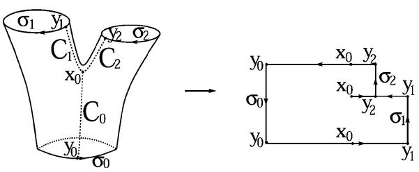
Mapping a Y-shaped vessel onto a plane. (After [24] © 2002 IEEE.)

The construction of the conformal mapping begins by finding the real part of f = u + iv. This is done by solving the Dirichlet problem Δu = 0 on Σ\(σ₀ ⋃ σ₁ ⋃ σ₂), with appropriate boundary conditions on σ₀, σ₁ and σ₂. The determination of the boundary conditions will be discussed in Section IV.

There is a well-known classical mathematical method for flattening a multiply-connected surface; see [14] and the references therein. The method involves solving the Dirichlet problem for each boundary component, then solving a simple linear system of equations to find the correct linear combination u of these functions, together with boundary conditions for its harmonic conjugate v. However, while mathematically elegant, we have found that the resulting mapping significantly distorts area. We adjust this algorithm to provide a mapping which is more practical for the purposes of medical visualization.

Analytically, there is a saddle point (also called a branch-point) x₀ on the surface where u’(x₀) = 0. We define three smooth curves C₀, C₁ and C₂ running from x₀ to σ₀, σ₁, and σ₂, respectively (Fig. 1), such that C₁ and C₂ are along the gradient direction of u and C₀ is opposite to the gradient direction of u. The curve C_i meets the boundary σ_i at point y_i(i = 0, 1, 2). Since u’(x₀) = 0, we can make C₁ and C₂ lie on a line in the neighborhood of x₀, while C₀ is perpendicular to the line.

These curves define a cut on Σ. The cut and the original boundaries σ₀, σ₁ and σ₂ define an oriented boundary B of the cut surface

$$y_0\stackrel{{\sigma }_0}{\to }{y}_0\stackrel{-C_0}{\to }{x}_0\stackrel{C_1}{\to }{y}_1\stackrel{{\sigma }_1}{\to }{y}_1\stackrel{-C_1}{\to }{x}_0\stackrel{C_2}{\to }{y}_2\stackrel{{\sigma }_2}{\to }{y}_2\stackrel{-C_2}{\to }{x}_0\stackrel{C_0}{\to }{y}_0$$

where –C_i implies that the boundary is oriented in the opposite direction of C_i.

The second step of constructing the mapping function is to calculate the harmonic conjugate of u by solving another Dirichlet problem Δv = 0. By the Cauchy-Riemann equations, we have

$$\frac{\partial v}{\partial s}=\frac{\partial u}{\partial n}$$ (1)

on B, and so the boundary condition of v satisfies

$$v\left(\zeta \right)={\int }_{{\zeta }_0}^{\zeta }\frac{\partial v}{\partial s}ds={\int }_{{\zeta }_0}^{\zeta }\frac{\partial u}{\partial n}ds$$ (2)

where ζ₀ is a given start point and ζ is any point on the boundary. The proof that the mapping is one-to-one (except on the branch-point) can be found elsewhere [14].

III. Numerical Method for Conformal Mappings

In Section II, we sketched the analytic approach for solving the conformal mapping problem on a Y-shaped tube. Here, we discuss the finite element method for finding an approximation to this mapping. See [12] for more details about this technique. The numerical method for finding the harmonic skeleton in Section IV is very similar to the method used here, with the specification of more boundary conditions. Related methods have been applied for brain flattening and colon flattening [2], [8]. The method used for vessel flattening is similar to these. However, due to the differences in topology, the boundary conditions have to be changed.

We now present the finite element method used to implement our flattening procedure. In this section, Σ is assumed to be a triangulated surface of a Y-shaped tube with three separate boundary components σ₀, σ₁ and σ₂. Let PL(Σ) denote the finite dimensional space of piecewise linear functions on Σ. A basis {φ_V} is defined on PL(Σ) such that for each vertex there is a corresponding piecewise linear basis function, which is 1 on this vertex and 0 on all other vertices, i.e.,

$$\begin{array}{cc}\hfill {\varphi }_V\left(V\right)=& 1\hfill \\ \hfill {\varphi }_V\left(W\right)=& 0,W\ne V\hfill \\ \hfill {\varphi }_V& \text{is linear on each triangle}.\hfill \end{array}$$ (3)

Any function u ∈ PL(Σ) can be approximated as the linear combination of these basis functions. The coefficients u_V are the values on vertices

$$u=\sum _V{u}_V{\varphi }_V.$$ (4)

The u we are seeking is continuous on Σ and piecewise linear on each triangle. From the classic theory of calculus of variations [17], it is known that the solution of the Laplace equation Δu = 0 is a harmonic function which minimizes the Dirichlet functional

$$\begin{array}{cc}\hfill D\left(u\right)=& \frac{1}{2}\int {\int }_{\Sigma }{\mid \nabla u\mid }^{2}dS,\hfill \\ \hfill u\mid \partial u_0=& {\alpha }_0,u\mid \partial u_1={\alpha }_1,u\mid \partial u_2={\alpha }_2.\hfill \end{array}$$ (5)

It can be proved [2] that u is the minimizer of the Dirichlet functional, if for each vertex Σ\(σ₀⋃σ₁⋃σ₂)

$$\sum _{W\in \Sigma \backslash ({\sigma }_0\cup {\sigma }_1\cup {\sigma }_2)}{D}_{VW}{u}_W=-\sum _{i=0,1,2}{\alpha }_i\sum _{W\in {\sigma }_i}{D}_{VW}.$$ (6)

D_VW is defined as

$$D_{VW}=\int \int \nabla {\varphi }_V\cdot \nabla {\varphi }_{W}dS$$ (7)

for any pair of vertices V and W.

Obviously, D_VW = 0 unless V and W are connected by an edge in the triangulation. Suppose VW is an edge belonging to two triangles VWX and VWY (Fig. 2). It is easy to show that for V ≠ W

$$D_{VW}=-\frac{1}{2}(\cot \angle X+\cot \angle Y)$$ (8)

where ∠X is the angle at the vertex X in the triangle VWX, and ∠Y is the angle at the vertex Y in the triangle VWY, as shown in Fig. 2. Further, we have

$$D_{VV}=-\sum _{W\ne V}{D}_{VW}$$ (9)

for V = W.

Fig. 2.

Triangle geometry.

What we are seeking is a flattening function f = u + iv. The computation for v is similar to that of u, using the boundary condition obtained from (2), which is derived from the Cauchy-Riemann equations.

IV. Harmonic Skeleton and Flattening of Multi-Branched Vessels

In this section, we will show how the conformal mapping algorithm can be extended to multibranched surfaces. The basic idea is to construct a skeleton of the branched vessel surface and to use this skeleton as a guide for dividing the whole surface into several Y-shaped tubes. Then the previously discussed mapping algorithm can be applied to each Y-shaped segment.

A number of algorithms have been considered for extracting a central line from a tubular surface. For example, the skeleton may be calculated by a “peeling the onion” technique, and is used as the central line [11]. However, the skeleton thus generated may not be smooth. Our method for extracting the central line is based on the solution of a harmonic equation on the tubular surface. Hence, we call it a “harmonic skeleton.” The harmonic skeleton is easy to compute and is guaranteed to be smooth. It can also automatically provide a viewing vector when used as the central line for fly-throughs. In addition, this algorithm can automatically provide the boundary conditions needed for the Dirichlet problem.

Again, let Σ denote an embedded surface (no self-intersections), which is topologically a tube with several branches. Each branch has boundary σ_i(i = 0, …, N), which is a topological circle.

The first step of the central line calculation is to solve the Dirichlet problem Δu = 0 on Σ\σ_i(i = 0, …, N) with appropriate boundary conditions. In our approach, we are working on a triangulated representation of Σ. One of the boundaries is designated to be the root, which can be selected arbitrarily or selected based on physiological considerations. The value of u on the root boundary is taken to be 0. We then perform the following region growing algorithm on the surface in order to determine the value of other boundaries:

1. mark the points on the root as “used” points;

2. mark all the neighbors of “used” points as “used” points;

3. step Number = step Number + 1;

4. repeat 2) & 3) until “used” points hit another boundary (target boundary);

5. set the value of target boundary as stepNumber.

In other words, we set a boundary’s value to be the number of triangles between the target boundary and the root boundary.

The second step is to build a tree-like structure, i.e., the harmonic skeleton. For a given u, we find all points on the surface with values equal to u(by interpolation). We then partition these points into several groups according to their positions on the surface. The centroid of each group corresponds to a point on the harmonic skeleton. By increasing from u 0 to the maximum value, we can build a structured tree. The locations of the bifurcations become obvious since it is easy to track where one circle splits into two.

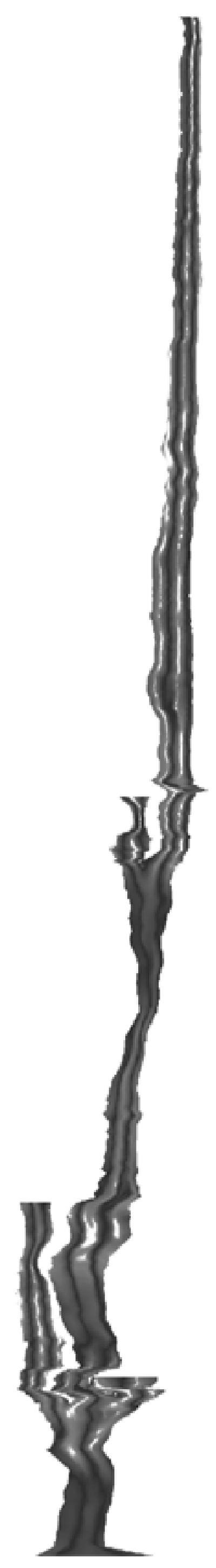
The third step is to refine the harmonic skeleton. In the first step, the boundary values are decided by triangle counts between the root and the other boundaries. This is a very coarse estimation. Now, we update them using the length of the preliminary harmonic skeleton, which is obtained in the second step. Then we solve the Dirichlet problem Δ u = 0 again and repeat the tree-extraction procedure (the second step) to get a refined harmonic skeleton. An example of a harmonic skeleton is shown in Fig. 3.

Fig. 3.

Harmonic skeleton for Fig. 4. (After [24] © 2002 IEEE.)

In applications such as virtual endoscopy and vessel crosssectional area measurement, we may also be interested in defining a forward direction for the camera. One straightforward method is to use the position differences of an ordered set of points on the skeleton. However, this often causes problems near bifurcations where the direction vector changes rapidly. This problem can be handled by using the singular value decomposition (SVD) [16]. When calculating the centroids in the second step, we can also do an SVD for each point group and choose the eigenvector associated with the smallest eigenvalue as the direction vector.

From the “tree” structure of the harmonic skeleton (Fig. 3), we can easily identify curve points, branch-points and end points. Ordinary curve points are connected to 2 points, branchpoints are connected to 3 points and end points are connected to only 1 point. This “tree” is then cut into several segments, each containing a Y-shaped structure. By using this partitioned skeleton as a reference, we can easily divide the whole vessel into several parts, each having only one branch-point.

The harmonic function u on the whole surface is found while building the harmonic skeleton. Next, cuts are made on each segment, and we solve for v (see Section II). Modifications are made to cuts where two segments meet. These modifications guarantee the mapping result is continuous on the whole surface.

V. Area-Preserving Mappings

The mappings constructed so far preserve angles. However, they are not area-preserving in general, since a flattening map to the plane cannot be both angle-preserving and area-preserving unless the original surface has zero Gaussian curvature. Some areas may be greatly enlarged or shrunk. This problem becomes particularly pronounced when we wish to construct a flattened representation for a multibranched surface. In a conformal representation, each time a vessel passes a branch point, it narrows approximately by a factor of two. In other words, the vessel at any point has approximately narrowed by a factor of 2^N, where N is the number of branch-points from the root. Hence, it may be interesting and useful to consider another type of one-to-one mapping that preserves areas instead of angles. In this section, we show how to use the theory of optimal mass transport to construct such an area-preserving mapping from the output of the conformal mapping algorithm. Here, we summarize the procedure; more technical details and a mathematical proof may be found in [9] and [23] and in the Appendix.

Assume we have the result for the conformal mapping f, which has range range(f) in the plane. We define a pseudodensity μ₀ on range(f) to be the area of a triangle on the original surface divided by the area of the triangle once flattened. The function μ₀ is extended to a rectangular region Ω₀ surrounding range(f) by setting μ₀ to a constant everywhere outside of range(f). The constant can be the mean of μ₀ inside range(f), or it can be several times the mean. Fig. 6 shows such a function μ₀. The dark color represents enlarged areas and the light color represents shrunken areas.

Fig. 6.

Area change ratio. (After [23] © 2003 Springer-Verlag.)

The target density map μ₁ is 1 everywhere on another rectangular region Ω₁, such that

$${\int }_{{\Omega }_0}{\mu }_0={\int }_{{\Omega }_1}{\mu }_1.$$ (10)

We find a mass preserving (MP) mapping function u from (Ω₀, μ₀) to (Ω₁, μ₁) such that

$${\mu }_0=\mid Du\mid {\mu }_1\circ u.$$ (11)

There exist many such mappings, however, we want to find an optimal one in the following sense: we minimize the functional

$$d{({\mu }_0,{\mu }_1)}^2=\int {\mid \mid u\left(x\right)-x\mid \mid }^2{\mu }_0\left(x\right)dx.$$ (12)

This is called the L² Monge-Kantorovich (MK) problem. This functional puts a penalty on the distance the map u moves each bit of material, weighted by the material’s mass. A fundamental theoretical result [7] shows there exists a unique optimal solution $\tilde{u}$, characterized as the gradient of a convex function (i.e., $\tilde{u}=\nabla w$).

Since μ₁=1, the constraint (11) reduces to ${\mu }_0=D\tilde{u}$, and so the mapping $\tilde{u}$ compensates exactly for the distortion in area which occurs during conformal flattening. Furthermore, since we minimize the functional (12) to find the optimal, our solution differs minimally from the identity.

The algorithm for finding the optimal mapping consists of finding an initial mapping u⁰, and then removing the curl of u⁰.

A. Finding an Initial Mapping

In principal, we can use any initial mass-preserving bijection. Since we are working on rectangular domains, the initial mapping can be constructed as follows. Set u⁰(x, y) = (a(x), b(x, y)). We can find a(x) by solving the equation

$${\int }_0^{a\left(x\right)}{\int }_0^{1}m{u}_1(\eta ,d\zeta )d\zeta d\eta ={\int }_0^x{\int }_0^1{\mu }_0(\eta ,\zeta )d\zeta d\eta$$ (13)

which is a one-dimensional (1-D) problem. In turn, b(x, y) may be found by solving

$$a^{\prime }\left(x\right){\int }_0^{b(x,y)}m{u}_1\left(a\right(x),\zeta )d\zeta ={\int }_0^y{\mu }_0(x,\zeta )d\zeta$$ (14)

which is a family of 1-D MK problems, each corresponding to a given x. Since we assume μ₀ and μ₁ are positive everywhere, a(x) is well-defined and strictly monotonically increasing, and b(x, y) is also well-defined and strictly monotonically increasing with respect to y. By construction, this initial mapping satisfies (11) and is guaranteed to be bijective.

B. Removing the Curl

Here, we will only briefly describe our iterative method; full details may be found in the Appendix. According to the theory of polar factorization [3], this initial mapping u⁰ can be factored as

$$u^0=(\nabla w)\circ \tilde{s}$$ (15)

where $\tilde{s}$ is an MP mapping from (Ω₀, μ₀) to itself.

The goal is to find the optimal MP mapping $\tilde{u}=\nabla w$. We consider the family of MP mappings in the form of u = u⁰○ s⁻¹, where s and its inverse function s⁻¹ are MP mappings from Ω₀ to Ω₀. Rather than do the polar factorization directly, we find it via a gradient descent method.

A mapping u (regarded as a vector field) may be expressed as the sum of two parts,

$$\begin{array}{cc}\hfill u=& \nabla w+\chi \hfill \\ \hfill \mathrm{div}\left(\chi \right)=& 0\text{and}\langle \chi ,\overrightarrow{n}\rangle =0\text{on}\partial {\Omega }_0\hfill \end{array}$$ (16)

where $\overrightarrow{n}$ is the normal to the boundary of Ω₀. In other words, the vector field u may be decomposed into two vector fields: one curl-free and the other divergence-free. The idea is to start with an initial MP function, u = u⁰, and evolve it in such a way as to kill the curl. In the two-dimensional case, the divergence-free vector field part can be written as χ = ∇^⊥f, where ∇^⊥f := (−f_y, f_x). The function f can be found by solving a Dirichlet boundary problem

$$\begin{array}{cc}\hfill -\mathrm{div}\left(u^{\perp }\right)=& \Delta f,\hfill \\ \hfill f=& 0\text{on}\partial {\Omega }_0.\hfill \end{array}$$ (17)

The evolution equation for u (see the Appendix below) is given by

$$u_t=\frac{1}{{\mu }_0}Du{\nabla }^{\perp }{\Delta }^{-1}\mathrm{div}\left(u^{\perp }\right)$$ (18)

which may be derived via a straightfoward gradient descent method. In practice, we update u iteratively until the curl goes below a certain predefined threshold.

VI. Implementation and Examples

We have tested our mapping algorithms on several datasets, and three of them are presented here. Please visit http://www.bme.gatech.edu/groups/minerva/publications/papers/zhu-tmi2004-color.pdf for color figures. All the programs were written in Matlab, partly using mex functions. Typically, the running time for a data set is approximately 30 min on a P4 3 GHz Linux computer, with 10 min for conformal mapping and 20 min for an area-preserving mapping.

The segmentation algorithm we used is a knowledge-based approach [21], which is similar to the method by Hernandez et al. [10]. In our algorithm, each voxel is assumed to be belong to one of several classes. A priori knowledge of each class is introduced by Bayes’ rule. Posterior probabilities obtained from Bayes’ rule are anisotropically smoothed, and the segmentation is obtained via the maximum a posteriori (MAP) classifications of the smoothed posteriors. An active contour model [5], [13] is applied to the blood class, and the desired arteries are extracted with subvoxel accuracy. This surface is then smoothed using a version of the mean curvature flow. The vessel caps are removed to generate an open-ended vessel surface.

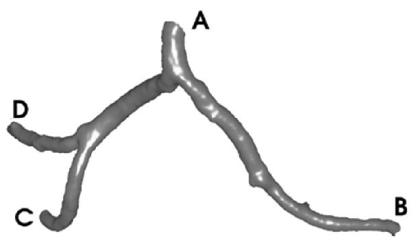
The first data set is a 256 × 256 × 47 brain MRA image provided by the Surgical Planning Lab of Brigham and Women’s Hospital. First, a triangulated representation of the frontal cerebral artery was obtained. Next, as described in Section IV, we generated the harmonic skeleton for the vessel, partitioned it, and assigned a boundary value to each end point. By using this partitioned skeleton as a reference, several sections of Y-shaped tubes were obtained. (In this dataset, the original vessel was partitioned into three Y-shaped sections.) Then, as described in Section II, the mapping function was solved for each Y-shaped section. The mapping results of all segments were put together to provide a, entire view of the vessel surface. We made some corrections where two Y-shaped sections meet, in order to make the flattened surface continuous. Finally, we made area preserving corrections on the conformal mapping result, and we generated a mapping that preserves area as described in Section V. In Fig. 4, an open-ended triangulated vessel surface is shown. The conformal mapping result is shown in Fig. 5(a), where the vertices have been assigned outward normals according to their original positions as seen in Fig. 4. The area change of this conformal mapping is shown in Fig. 6. As we have stated before, a light color indicates a shrinkage of area, and a dark color indicates a dilation. The initial mapping u⁰ for the area-preserving mapping is shown in Fig. 7, and the final area-preserving mapping is shown in Fig. 5(b). The corresponding locations between Figs. 4 and 5 are indicated by capital letters.

Fig. 4.

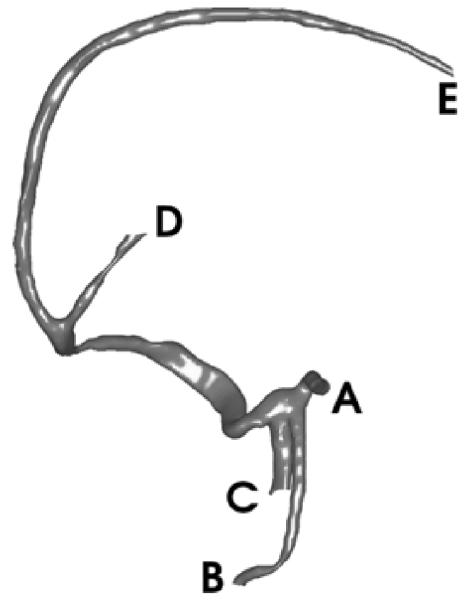
Original brain vessel. (After [23] © 2003 Springer-Verlag.)

Fig. 5.

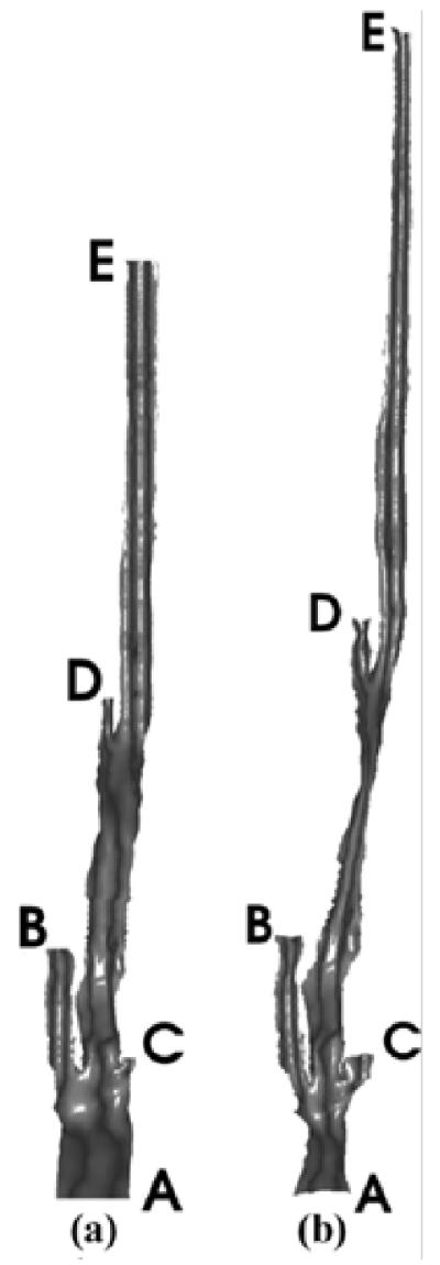
Flattened brain vessel shaded by original normal vectors. (a) Conformal mapping, (b) Area-preserving mapping. (After [23] © 2003 Springer-Verlag.)

Fig. 7.

The initial mapping for area-preserving mapping.

The second example is a coronary artery data set including left main coronary artery, LAD and LCX. This 512 × 512 × 200 set came from the Department of Radiology of Emory Hospital. The original surface of the coronaryartery is shownin Fig.8, and mapping results are presented in Fig. 9. Again, vertices have been assigned outward normals according to their original positions.

Fig. 8.

Original coronary artery.

Fig. 9.

Flattened coronary artery shaded by original normal vectors. (a) Conformal mapping, (b) Area-preserving mapping.

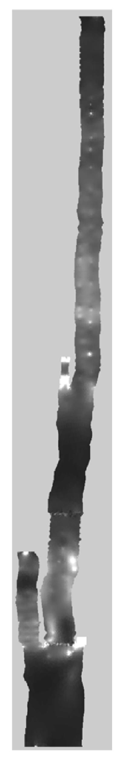
The last example is a 512 × 512 × 80 carotid artery dataset. By using the method described above, we generated its anglepreserving representation as well its area-preserving representation. In this case, there is only one Y-shaped structure (Fig. 10). The results from the two types of mappings are shown in Fig. 11. The surfaces are shaded by the computed axial wall shear stress (WSS) in dyne/cm². Regions with dark blue colors (indicating low axial WSS) correlate with atherosclerosis [22]. The histogram of area change in the conformal mapping is presented in Fig. 12, in which x axis represents the area changing ratios of triangles and y axis represents the number of triangles. We can see that most of the triangles have area changing ratios ranging from 0.3 to 2. After area corrections, the area changing ratios are from 0.8 to 1.1 for most triangles (Fig. 13). The ratios are not exactly 1 due to some numerical errors. Other geometric quantities, such as the cross-sectional area of vessels or the level of calcification can also be visualized in this manner.

Fig. 10.

Original carotid artery shaded by wall shear stress.

Fig. 11.

Flattened carotid artery shaded by wall shear stress. (a) Conformal mapping, (b) Area-preserving mapping.

Fig. 12.

Statistics of area changing in conformal mapping for carotid artery.

Fig. 13.

Statistics of area changing in area-preserving mapping for carotid artery.

VII. Conclusion

In this paper, we presented two methods for flattening tubular branched surfaces (e.g., blood vessels). The first method is based on conformal geometry and harmonic analysis, which preserves angles and the local geometry. The second method is an area-preserving approach, which is based on the theory of optimal mass transport. In this case, we use Monge-Kantorovich theory to construct an area-preserving mapping starting with the conformal mapping derived via the first procedure. We have also proposed a “harmonic skeleton” method for calculating the “center line” for a highly-branched tubular surface. This method can be used in other applications such as virtual colonoscopy.

Optimal mass transport theory, which is used in the construction of area-preserving mappings, has other applications in medical imagery and computer vision more generally. For example, it is a natural technique for solving certain types of registration problems in functional MR, if one desires to compare the degree of activity in various features deforming over time and generate a corresponding elastic registration map. We are now developing new registration algorithms with such a mass-preserving constraint. In addition to the medical applications, we plan to apply this methodology to certain natural images for image morphing and optical flow.

APPENDIX

In this appendix, we present some mathematical details omitted in Section V. We mainly focus on the proof of some MP mappings properties and the deduction of our gradient descent method. Full details of the mathematics underlying our methodology (including convergence to the optimal solution) may be found in [1].

A. Properties of Mass Preserving Mappings

A simple calculation verifies that the composition of two mass preserving mappings is an MP mapping, and that the inverse of an MP mapping is also an MP mapping. Since u⁰ is an MP mapping, and u = u⁰ ○ s⁻¹, we see that u is an MP mapping if and only if s⁻¹ (and also s) is an MP mapping. Hence, s should satisfy

$${\mu }_0=\mid Ds\mid {\mu }_0\circ s.$$ (19)

Next, rather than working with directly, we solve the polar factorization problem via gradient descent. Accordingly, we take to be a function of pseudotime parameter t, and we try to find the gradient direction which will decrease the L² Monge-Kantorovich functional. In what follows, the t subscript denotes differentiation with respect to the pseudotime t, while the D, ∇ and div all refer to spatial derivatives.

By taking the derivative of (19) with respect to t, we get

$$\begin{array}{cc}\hfill 0=& {\mid Ds\mid }_t{\mu }_0\circ s+\mid Ds\mid {({\mu }_0\circ s)}_t\hfill \\ \hfill 0=& \mid Ds\mid \left(\mathrm{div}\right(s_t\circ s^{-1})\circ s){\mu }_0\circ s+\mid Ds\mid \langle (\nabla {\mu }_0)\circ s,s_t\rangle \hfill \\ \hfill 0=& \left({\mu }_0\mathrm{div}\right(s_t\circ s^{-1}\left)\right)\circ s+\langle (\nabla {\mu }_0)\circ s,s_t\rangle \hfill \\ \hfill 0=& {\mu }_0\mathrm{div}(s_t\circ s^{-1})+\langle \nabla {\mu }_0,s_t\circ s^{-1}\rangle \hfill \\ \hfill 0=& \mathrm{div}({\mu }_0{s}_t\circ s^{-1}).\hfill \end{array}$$

Hence, s_t should have the following form

$$s_t=\left(\frac{1}{{\mu }_0}\zeta \right)\circ s$$ (20)

for some vector field ζ on Ω₀, with div(ζ) = 0 and $\langle \zeta ,\overrightarrow{n}\rangle =0$ on ∂Ω₀, $\overrightarrow{n}$ being the normal to the boundary of Ω₀.

Since u⁰ = u ○ s, differentiating it with respect to t yields

$$\begin{array}{cc}\hfill (Du\circ s)s_t+u_t\circ s=& 0\hfill \\ \hfill u_t\circ s=& -(Du\circ s)s_t\hfill \\ \hfill u_t=& -Du{s}_t\circ s^{-1}.\hfill \end{array}$$

From (20), we have

$$u_t=-\frac{1}{{\mu }_0}Du\zeta$$ (21)

with ζ as above.

B. Gradient Descent Method for L² Monge-Kantorovich Problem

Consider now the problem of minimizing the L² Monge-Kantorovich functional:

$$M={\int }_{{\Omega }_0}{\mid \mid u-x\mid \mid }^2{\mu }_0$$ (22)

$$={\int }_{{\Omega }_0}{\mid \mid u\mid \mid }^2{\mu }_0-2{\int }_{{\Omega }_0}\langle u,x\rangle {\mu }_0+{\int }_{{\Omega }_0}{\mid \mid x\mid \mid }^2{\mu }_0.$$ (23)

The last term is obviously independent of time. Interestingly, so is the first term. To see this, we set y = s⁻¹(x), and using the MP property of s and s⁻¹, we find

$${\mu }_0\left(x\right)dx={\mu }_0\circ s\left(y\right)ds\left(y\right)={\mu }_0\circ s\left(y\right)\mid Ds\left(y\right)\mid dy={\mu }_0\left(y\right)dy$$ (24)

since μ₀(y) = μ₀ ○ s(y)|Ds(y). Now we have

$$\begin{array}{cc}\hfill {\int }_{{\Omega }_0}{\mid \mid u\left(x\right)\mid \mid }^2{\mu }_0\left(x\right)dx=& {\int }_{{\Omega }_0}{\mid \mid u^0\circ s^{-1}\left(x\right)\mid \mid }^2{\mu }_0\left(x\right)dx\hfill \\ \hfill =& {\int }_{{\Omega }_0}{\mid \mid u^0\left(y\right)\mid \mid }^2{\mu }_0\left(y\right)dy\hfill \end{array}$$

which is a constant for all t. Turning now to the middle term, we do the same trick by setting y = s⁻¹(x). Now we have

$$\begin{array}{cc}\hfill {\int }_{{\Omega }_0}\langle u\left(x\right),x\rangle {\mu }_0=& {\int }_{{\Omega }_0}\langle u^0\circ s^{-1}\left(x\right),s\circ s^{-1}\left(x\right)\rangle {\mu }_0\left(x\right)dx\hfill \\ \hfill =& {\int }_{{\Omega }_0}\langle u^0\left(y\right),s\left(y\right)\rangle {\mu }_0\left(y\right)dy\hfill \end{array}$$

and taking s_t = ((1/μ₀)ζ) ○ s, we compute

$$\begin{array}{cc}\hfill -\frac{1}{2}{M}_t=& {\int }_{{\Omega }_0}\langle u^0\left(y\right),s_t\left(y\right)\rangle {\mu }_0\left(y\right)dy\hfill \\ \hfill =& {\int }_{{\Omega }_0}\langle u\circ s\left(y\right),\left(\frac{1}{{\mu }_0}\zeta \right)\circ s\left(y\right)\rangle {\mu }_0\left(y\right)dy\hfill \\ \hfill =& {\int }_{{\Omega }_0}\langle u\left(x\right),\frac{1}{{\mu }_0\left(x\right)}\zeta \left(x\right)\rangle {\mu }_0\left(x\right)dx\hfill \\ \hfill =& {\int }_{{\Omega }_0}\langle u\left(x\right),\zeta \left(x\right)\rangle dx.\hfill \end{array}$$

Now decomposing u as u = ∇w + χ, we have

$$\begin{array}{cc}\hfill -\frac{1}{2}{M}_t=& {\int }_{{\Omega }_0}\langle \nabla w+\chi ,\zeta \rangle \hfill \\ \hfill =& {\int }_{{\Omega }_0}\langle \nabla w,\zeta \rangle +{\int }_{{\Omega }_0}\langle \chi ,\zeta \rangle \hfill \\ \hfill =& {\int }_{{\Omega }_0}\left(\mathrm{div}\right(w\zeta )-w\mathrm{div}(\zeta \left)\right)+{\int }_{{\Omega }_0}\langle \chi ,\zeta \rangle \hfill \\ \hfill =& {\int }_{\partial {\Omega }_0}w\langle \zeta ,n\rangle +{\int }_{{\Omega }_0}\langle \chi ,\zeta \rangle \hfill \\ \hfill =& {\int }_{{\Omega }_0}\langle \chi ,\zeta \rangle \hfill \end{array}$$

where we’ve used the divergence theorem, div(ζ) = 0 and $\langle \zeta ,\overrightarrow{n}\rangle =0$ on ∂Ω₀. Choosing ζ = χ, recalling χ = ∇^⊥ f, and using (17) and (21), it is easy to see that

$$u_t=\frac{1}{{\mu }_0}Du{\nabla }^{\perp }{\Delta }^{-1}\mathrm{div}\left(u^{\perp }\right)$$ (25)

which is the required gradient flow equation.

References

- [1].Angenent S, Haker S, Tannenbaum A. Minimizing flows for the Monge-Kantorovich problem. SIAM J. Math. Anal. 2003;35(1):61–97. [Google Scholar]
- [2].Angenent S, Haker S, Tannenbaum A, Kikinis R. On the Laplace-Beltrami operator and brain surface flattening. IEEE Trans. Med. Imag. 1999 Aug;18(8):700–711. doi: 10.1109/42.796283. [DOI] [PubMed] [Google Scholar]
- [3].Brenier Y. Polar factorization and monotone rearrangement of vectorvalued functions. Commun. Pure Appl. Math. 1991;64:375–417. [Google Scholar]
- [4].Carman G, Drury H, Essen DV. Computational methods for reconstructing and unfolding the cerebral cortex. Cerb. Cortex. 1995;5(6):506–517. doi: 10.1093/cercor/5.6.506. [DOI] [PubMed] [Google Scholar]
- [5].Caselles V, Kimmel R, Sapiro G. Geodesic active contours. Int. J. Comput. Vis. 1997;22(1):61–79. [Google Scholar]
- [6].Farkas H, Kra I. Riemann Surfaces. Springer-Verlag; New York: 1991. [Google Scholar]
- [7].Gangbo W, McCann R. The geometry of optimal transportation. Acta Math. 1996;177:113–161. [Google Scholar]
- [8].Haker S, Angenent S, Tannenbaum A, Kikinis R. Nondistorting flattening maps and the 3-D visualization of colon CT images. IEEE Trans. Med. Imag. 2000 Jul;19(7):665–670. doi: 10.1109/42.875181. [DOI] [PubMed] [Google Scholar]
- [9].Haker S, Tannenbaum A. Optimal mass transport and image registration; Proc. Workshop Variational and Level Set Methods in Computer Vision (VLSM’01); 2001.pp. 29–36. [Google Scholar]
- [10].Hernandez M, Frangi A, Sapiro G. Three-dimensional segmentation of brain aneurysms in CTA using nonparametric region-based information and implicit deformable models: Method and evaluation. In: Ellis RE, Peters TM, editors. Proc. Medical Image Computing and Computer-Assisted Intervention (MICCAI 2003) 2003. pp. 594–602. [Google Scholar]
- [11].Hong L, Kaufman A, Wei Y, Viswambharan A, Wax M, Liang Z. 3-D virtual colonoscopy. Proc. Biomedical Visualization (BIOMEDVIS’95) 1995:26–32. [Google Scholar]
- [12].Hughes T. The Finite Element Method. Prentice-Hall; Upper Saddle River, NJ: 1987. [Google Scholar]
- [13].Kichenasamy S, Olver P, Tannenbaum A, Yezzi A. Conformal curvature flows: From phase transitions to active contours. Arch. Rational Mech. Anal. 1996;134(3):275–301. [Google Scholar]
- [14].Nehari Z. Conformal Mapping. Dover; New York: 1975. [Google Scholar]
- [15].Paik D, Beaulieu C, Jeffrey R, Karadi C, Napel S. Visualization modes for CT colonography using cylindrical and planar map projections. J. Comput. Assist. Tomogr. 2000;24(2):179–188. doi: 10.1097/00004728-200003000-00001. [DOI] [PubMed] [Google Scholar]
- [16].Press W, Teukolsky S, Vetterling W, Flannery B. Numeircal Recipes in C. 2 ed. Cambridge Univ. Press; Cambridge: 1992. [Google Scholar]
- [17].Rauch J. Partial Differential Equations. Springer-Verlag; New York: 1991. [Google Scholar]
- [18].Schwartz E, Shaw A, Wolfson E. A numerical solution to the generalized mapmaker’s problem: Flattening noncovex polyhedral surfaces. IEEE Trans. Pattern Anal. Machine Intell. 1989 Sep;11(9):1005–1008. [Google Scholar]
- [19].Wang G, Dave S, Brown B, Zhang Z, McFarland E, Haler J, Vannier M. Colon unraveling based on electrical field—Recent progress and further work. Proc. SPIE (Medical Imaging 1999: Physiology and Function from Multidimensional Images) 1999;3660:125–132. [Google Scholar]
- [20].Wang G, McFarland E, Brown B, Vannier M. GI tract unraveling with curved cross sections. IEEE Trans. Med. Imag. 1998 Apr;17(2):318–322. doi: 10.1109/42.700745. [DOI] [PubMed] [Google Scholar]
- [21].Yang Y, Tannenbaum A, Giddens D. Knowledge-based 3-D segmentation and reconstruction of coronary arteries using CT images; presented at the IEEE EMBS04; San Francisco, CA. 2004; [DOI] [PubMed] [Google Scholar]
- [22].Zarin C, Giddens D, Bharadvaj B, Sottiurai V, Mabon R, Glagov S. Carotid bifurcation atherosclerosis: Quantitative correlation of plaque localization with flow velocity profiles and wall shear stress. Circ. Res. 1983;53(4):502–514. doi: 10.1161/01.res.53.4.502. [DOI] [PubMed] [Google Scholar]
- [23].Zhu L, Haker S, Tannenbaum A. Area-preserving mappings for the visualization of medical structures. In: Ellis RE, Peters TM, editors. Proc. Medical Image Computing and Computer-Assisted Intervention (MICCAI 2003) 2003. pp. 277–284. [Google Scholar]
- [24].Zhu L, Haker S, Tannenbaum A, Bouix S, Siddiqi K. Anglepreserving mappings for the visualization of multi-branched vessels; Proc. Int. Conf. Image Processing 2002 (ICIP2002); 2002.pp. 945–948. [Google Scholar]