Accurate Molecular Polarizabilities Based on Continuum Electrostatics

Abstract

A novel approach for representing the intramolecular polarizability as a continuum dielectric is introduced to account for molecular electronic polarization. It is shown, using a finite-difference solution to the Poisson equation, that the Electronic Polarization from Internal Continuum (EPIC) model yields accurate gas-phase molecular polarizability tensors for a test set of 98 challenging molecules composed of heteroaromatics, alkanes and diatomics. The electronic polarization originates from a high intramolecular dielectric that produces polarizabilities consistent with B3LYP/aug-cc-pVTZ and experimental values when surrounded by vacuum dielectric. In contrast to other approaches to model electronic polarization, this simple model avoids the polarizability catastrophe and accurately calculates molecular anisotropy with the use of very few fitted parameters and without resorting to auxiliary sites or anisotropic atomic centers. On average, the unsigned error in the average polarizability and anisotropy compared to B3LYP are 2% and 5%, respectively. The correlation between the polarizability components from B3LYP and this approach lead to a R² of 0.990 and a slope of 0.999. Even the F₂ anisotropy, shown to be a difficult case for existing polarizability models, can be reproduced within 2% error. In addition to providing new parameters for a rapid method directly applicable to the calculation of polarizabilities, this work extends the widely used Poisson equation to areas where accurate molecular polarizabilities matter.

1. Introduction

The linear response of the electronic charge distribution of a molecule to an external electric field, the polarizability, is at the origin of many chemical phenomena such as electron scattering¹, circular dichroism², optics³, Raman scattering⁴, softness and hardness⁵, electronegativity⁶, etc. In atomistic simulations, polarizability is believed to play an important and unique role in intermolecular interactions of heterogeneous media such as ions passing through ion channel in cell membranes⁷, in the study of interfaces⁸ and in protein-ligand binding⁹.

Polarizability is considered to be a difficult and important problem from a theoretical point of view. Much effort has been invested in the calculation of molecular polarizability at different levels of approximation. At the most fundamental level, electronic polarization is described by quantum mechanics (QM) electronic structure theory such as extended basis set density functional theory (DFT) and ab initio molecular orbital theory. However, the extent of the computational resources required is an impediment to the wide application of these methods on large molecular sets or on large molecular systems such as drug-like molecules¹⁰. In order to circumvent these limitations, empirical physical models based on classical mechanics have been parameterized to fit experimental or quantum mechanical polarizabilities.

In this article, we explore a new empirical physical model to account for electronic polarizability in molecules. The Electronic Polarization from Internal Continuum (EPIC) model uses a dielectric constant and atomic radii to define the electronic volume of a molecule. The molecular polarizability tensor is calculated by solving the Poisson equation (PE) with a finite difference algorithm. The concept that a dielectric continuum can account for solute polarizability has been examined previously. For example, Sharp et al.¹¹ showed that condensed phase induced molecular dipole moments are accounted for with the continuum solvent approach and that it leads to accurate electrostatic free energy of solvation. More recently Tan and Luo¹² have attempted to find an optimal inner dielectric value that reproduces condensed phase dipole moments in different continuum solvents. In spite of these efforts, we found that none of these models can account correctly for molecular polarizability. Here, the concept is explored with the objective of producing a high accuracy polarizable electrostatic model. Therefore, we focus on the optimization of atomic radii and inner dielectrics to reproduce the B3LYP/aug-cc-pVTZ polarizability tensor.

In this preliminary work, we seek to establish the soundness and accuracy of the EPIC model in the calculation of the molecular polarizability tensor on three classes of molecules: homonuclear diatomics, heteroaromatics and alkanes. These molecular classes required special attention with previous polarizable models due to their high anisotropy^13–15. Overall, 53 different molecules are used to fit our model and 45 molecules to validate the results. Six specific questions are addressed: Can the EPIC model accurately calculate the average polarizability? If so, can it further account for the anisotropy and the orientation of the polarizability components? How few parameters are needed to account for highly anisotropic molecules and how does this compare to other polarizable models? How transferable are the parameters obtained with this model? Is the model able to account for conformational dependency? In answering these questions, we obtained a fast and validated method with optimized parameters to accurately calculate the molecular polarizability tensor for a large variety of heteroaromatics not previously considered.

The remainder of the article is organized as follows. In the next section, we briefly review the most successful existing polarizable approaches, focusing on aspects relevant to this study. Then we introduce the dielectric polarizable method with a polarizable sphere analytical model. A methodology section in which we outline the computational details follows. The molecular polarizability results are then reported. This is followed by a discussion and conclusion.

2. Existing Empirical Polarizable Models

2.1 Point Inducible Dipole

The point inducible dipole model (PID) was first outlined by Silberstein in 1902¹⁶. This model has been extensively used to calculate molecular polarizability^{14,15,17–22} and to account for many-body effects in condensed phase simulations^23–25. Typically, in the PID, an atom is a polarizable site where the electric field direction and strength together with the atomic polarizability define the induced atomic dipole moment. Since the electric field at an atomic position is in part due to other atoms’ induced dipoles, the set of equations must be solved iteratively (or through a matrix inversion). In 1972, Applequist¹⁹ showed that the PID can accurately reproduce average molecular polarizability of a diverse set of molecules, but also that the mathematical formulation of the PID can lead to a polarizability catastrophe. Briefly, when two polarizable atoms are close to each other, the solution to the mathematical equations involved is either undetermined (with the matrix inversion technique) or the neighboring dipole moments cooperatively increase to infinity. To circumvent this problem, Thole^14,22 modified the dipole field tensor with a damping function, which depends on a lengthscale parameter meant to represent the spatial extent of the polarized electronic clouds; his proposed exponential modification is still important and remains in use^13,14,26.

2.2 Drude Oscillators

The Drude oscillator (DO) represents electronic polarization by introducing a massless charged particle attached to each polarizable atom by a harmonic spring²⁷. When the Drude charge is large and tightly bound to its atom, the induced dipole essentially behaves like a PID. The DO model is attractive because it preserves the simple charge-charge radial Coulomb electrostatic term already present and it can be used in molecular dynamics simulation packages without extensive modifications. The DO model has not yet been extensively parameterized to reproduce molecular polarizability tensors, but recent results suggest that it could perform as well as PID methods. Finally, the DO model also requires a damping function to avoid the polarizability catastrophe²⁶.

2.3 Fluctuating Charges

A third class of empirical model, called fluctuating charge (FQ), was first published in a study by Gasteiger and Marsili²⁸ in 1978 to rapidly estimate atomic charges. Subsequently, FQ was adapted to reproduce molecular polarizability and applied in molecular dynamic simulations^29,30. It is based on the concept that partial atomic charges can flow through chemical bonds from one atomic center to another based on the local electrostatic environment surrounding each atom. The equilibrium point is reached when the defined atomic electronegativities are equal. The FQ model, like the DO, has mainly been used in condensed phase simulations and not specifically parameterized to reproduce molecular polarizabilities. A major problem with FQ is the calculation of directional polarizabilities (eigenvalues of the polarizability tensor). For planar or linear chemical moieties (ketones, aromatics, alkane chains, etc.) the induced dipole can only have a component in the plane of the ring or in line with the chain. For instance, the out-of-plan polarizability of benzene can only be correctly calculated if out-of-plane auxiliary sites are built. For alkane chains, though, there is no simple solution³¹. For this reason, the ability of the FQ model to accurately represent complex molecular polarizabilities is clearly limited.

2.4 Limitations with the PID related methods

The PID and the related models have been parameterized and show an average error on the average polarizability around 5%. However, errors in the anisotropy are often around 20% or higher^15,20. Diatomic molecules are not handled correctly by any of these methods leading to errors of 82% in the anisotropy for F₂ for example^13,14. Heteroaromatics, which are abundant moities in drugs, are often poorly described by PID methods. This limitation is due to the source of anisotropy in the PID model i.e. the interatomic dipole interaction located at static atom positions. It is nevertheless possible to improve these models. For example, using full atomic polarizability tensors instead of isotropic polarizabilities have reduced the errors in polarizability components from 20% to 7%^20,21. In the case of the DO model, acetamide polarizabilities have been corrected by the addition of atom-type-dependent damping parameters and anisotropic harmonic springs³². In these cases, the improvement required a significant amount of additional parameters which brings an additional level of difficulty in their generalization. As illustrated below, our model seems to address most of these complications without additional parameters and complexity.

3. Dielectric polarizability model

The mathematical model that we explore in this article is based on simple concepts that have proved extremely useful in chemistry^33–38. We propose a specific usage that we clarify and describe in this section.

3.1 The model

Traditionally in Poisson-Boltzmann (PB) continuum solvent calculations, the solute is described as a region of low dielectric containing a set of distributed point charges; the polar continuum solvent (usually water) is described by a region of high dielectric. This theoretical approach gives the choice to either include average solution salt effects (PB) or to use the pure solvent (PE). Solving PE for such a system is equivalent to calculating a charge density around the solute surface at the boundary where the dielectric changes³⁹. This, among other things, allows the calculation of the free energy of charging of a cavity in a continuum solvent where, at least in the case of water, polarization comes mostly from solvent nuclear motion average. While the dielectric boundary is de facto representing the molecular polarization, the dielectric constants and radii employed traditionally are parameterized by fitting to energies (such as solvation or binding free energies) without regard for the molecular polarizabilities themselves. These energies are also dependent on details of the molecular electronic charge distribution, the solvent/solute boundary, and sometimes the nonpolar energy terms, all of which obfuscate the parameterization with respect to the key property of molecular polarizability.

Our approach is to use an intramolecular effective dielectric constant, together with associated atomic radii, to accurately represent the detailed molecular polarizability. For this to be a widely applicable model of polarizability, the generality between related chemical species of a given set of intramolecular effective dielectric constants and associated atomic radii would have to be demonstrated. Such a polarizability model, independent per se of the molecule’s charge distribution, could then subsequently be combined with a suitable static charge model to produce a polarizable electrostatic term applicable to force fields.

To evaluate the model, the simplest starting point is gas-phase polarizabilities, using a higher dielectric value inside the molecule and vacuum dielectric outside⁴⁰. This way, the charge density formed at the exterior/interior boundary comes from the polarization of the molecule alone. Comparison of the polarizability tensors from such calculations directly to those from B3LYP/aug-cc-pVTZ calculations allows proof-of-concept of the model. The resulting parameters can be used to rapidly calculate molecular polarizabilities on large molecules.

To calculate the molecular polarizability, we first solve EPIC for a system in which the interior/exterior boundary is described by a van der Waals (vdW) surface, an inner dielectric and a uniform electric field. The electric field is simply produced from the boundary conditions when solving on a grid (electric clamp). From the obtained solution, it is possible to calculate the charge density from Gauss’ law (i.e. from the numerical divergence of the electric field) and the induced dipole moment is simply the sum of the grid charge times its position as shown by eqn 1 below.

$${\stackrel{\rightharpoonup }{\mu }}^{\mathit{ind}}=\sum _{i=1}^{\mathit{grid}}{\stackrel{\rightharpoonup }{r}}_i·q_i$$ 1

Knowing the applied electric field, it is then possible, as shown in eqn 2, to compute the polarizability tensor given that three calculations are done with the electric field applied in orthogonal directions; in eqn 2, i and j can be x, y or z.

$${\alpha }_{ij}={\mu }_i^{\mathit{ind}}/E_j$$ 2

3.2 Spherical dielectric

For the sake of clarifying the internal structure of the model, let us first consider the induced polarization of a single atom in vacuum under the influence of a uniform external electric field – the EPIC model for an atom. Given a sphere of radius R, a unitless inner dielectric ε_in and the uniform electric field E, we can exactly calculate the induced dipole moment with eqn 3.

$${\stackrel{\rightharpoonup }{\mu }}^{\mathit{ind}}=4\pi {\epsilon }_0\left(\frac{{\epsilon }_{in}-1}{{\epsilon }_{in}+2}\right)R^3·\stackrel{\rightharpoonup }{E}$$ 3

Here, the atomic polarizability is given by the electric field E pre-factor, which is a scalar given the symmetry of the problem. The induced dipole moment originates from the accumulation of a charge density at the boundary of the sphere opposing to uniform electric field³⁹. From eqn 3, we see that the polarizability has a cubic dependency on the sphere radius and that the inner dielectric can reduce the polarizability to zero (ε_in=1), while the upper limit of its contribution is a factor of 1 (ε_in ≫ 1). The contribution of ε_in to the atomic polarizability asymptotically reaches a plateau as shown in Figure 1. Thus at high values of ε_in, the atomic radius becomes the dominant dependency in the electric field pre-factor; we find similar characteristics for non-spherical shapes.

Figure 1.

The dielectric contribution to the sphere dielectric continuum polarizability goes asymptotically to one and most of the contributions are below ε_in = 10.

It is interesting to make a parallel between eqn 3 and the PID model, where the polarizable point would be located exactly at the nucleus. In this particular case, it is possible to equate the polarizability from PE, induced by the radius and the dielectric, to any point polarizability¹¹. However, when the electric field is not uniform, the PID induced atomic dipole originating from the evaluation of the electric field at a single point may not be representative, leading to inaccuracies⁴¹. This is in contrast with the EPIC model that builds the response based on the electric field lines passing locally through each part of the atom’s surface, allowing a response more complex than that of a point dipole. In molecules, the atomic polarizabilities of the PID model do not find their counterparts in the EPIC model since it is difficult to assign non-overlapping dielectric spheres to atoms and obtain the correct molecular behavior. The Cl₂ molecule studied in this work is an example.

4. Methods

4.1 Calculations

Prior to the DFT calculation, SMILES^42–44 strings of the desired structures were transformed into hydrogen-capped three-dimensional structures with the program OMEGA⁴⁵. The n-octane conformer set was also obtained from OMEGA. The resulting geometries were optimized with the Gaussian’03⁴⁶ program using B3LYP^47–49 with a 6–31++G(d, p) basis set^50,51 without symmetry. The atomic radii and molecular inner dielectrics were fit based on molecular polarizability tensors calculated at the B3LYP level of theory⁵² with the Gaussian’03 program. The extended Dunning’s aug-cc-pVTZ basis set^53,54, known to lead to accurate gas phase polarizabilities, was used⁵⁵. An extended basis set is required to obtain accurate gas phase polarizabilities that would otherwise be underestimated.

The solutions to the PE were obtained with the finite difference PB solver Zap⁵⁶ from OpenEye Inc. modified to allow voltage clamping of box boundaries to create a uniform electric field. The electric field is applied perpendicularly to two facing box sides (along the z axis). The difference between the fixed potential values on the boundaries is set to meet: Δϕ = E_z × ΔZ, where Δϕ is the difference in potential, E_z is the magnitude of the uniform electric field and ΔZ is the grid length in the z direction. The salt concentration was set to zero and the dielectric boundary was defined by the vdW surfaces. The grid spacing was set to 0.3 Å and the extent of the grid was set such that at least 5 Å separated the box wall from any point on the vdW surface. As detailed in the Supporting Information, grid spacing below 0.6 Å did not show significant deterioration of the results. Small charges of ±0.001e were randomly assigned to the atoms to ensure ZAP would run, typically converging to 0.000001 kT.

In tables where optimized parameters are reported, a sensitivity value associated with each fitted parameter is also reported. The sensitivity of a parameter corresponds to its smallest variation producing an additional 1% error in the fitness function considering only molecules using this parameter. The sensitivity is calculated with a three-point parabolic fit around the optimal parameter value and the change required obtaining the 1% extra error is extrapolated. Therefore, the reported sensitivity indicates the level of precision for a given parameter and whether or not some parameters could be eventually merged.

4.3 Fitting procedure

Eqn 4 shows the fitness function F utilized in the fitting of the atomic radii, and the inner dielectrics.

$$F(\{R\},\{\epsilon \})=\frac{1}{3N}\sum _{i=1}^N\sum _{j=xx,yy,zz}\frac{\mid {\alpha }_{ij}^{QM}-{\alpha }_{ij}\mid }{{\alpha }_{ij}^{QM}}+\frac{1}{N_{\theta }}\sum _{i=1}^{N_{\theta }}\frac{1-\left|{\stackrel{\rightharpoonup }{v}}_{ij}^{QM}·{\stackrel{\rightharpoonup }{v}}_{ij}\right|}{1-cos45°}$$ 4

In eqn 4, N corresponds to the number of molecules used in the fit, α_ij to the polarizability component j of the molecule i and ν_ij to the eigenvector of the polarizability component j of molecule i. N_θ is the number of non-degenerate eigenvectors found in all the molecules. This fitness function is minimal when the three calculated polarizability components are identical to the QM values and when the corresponding component directions are aligned with the QM eigenvectors of the polarizability tensor.

As shown in the Cl₂ example of Figure 2, the hypersurface of eqn 4 has a number of local minima; it is important that our fitting procedure allows these to be examined. Because the calculations were fast, we decided to proceed in two steps: First, a systematic search was carried out varying each fitted parameter over a range and testing all combinations. The 30 best sets of parameters were then relaxed using a Powell minimization algorithm and the set of optimized parameters leading to the smallest error was kept.

Figure 2.

The EPIC model behavior is explored for Cl₂. The average polarizability (a) and the anisotropy (b) isolines (in a.u.) are plotted as a function of the Cl atomic radius, used to define the vdW surface, and the value of the inner dielectric. The target Cl₂ B3LYP values are 31.43 (average) and 18.24 (anisotropy) (c.f. Table 1). The polarizability tensor error function $(2\mid {\alpha }_{\perp }^{QM}-{\alpha }_{\perp }^{\mathit{EPIC}}\mid +\mid {\alpha }_{\left|\right|}^{QM}-{\alpha }_{\left|\right|}^{\mathit{EPIC}}\mid )/3{\alpha }_{\mathit{avg}}^{QM}$ isolines in (c) identify the regions where the EPIC model matches the B3LYP polarizability tensor. The external dielectric is set to one and the inter-nuclear distance of Cl₂ is fixed at 2.05Å. These figures show that a high dielectric value is required to match the QM anisotropy, and that a number of minima can be found on the error hypersurface.

4.4 Definitions

The polarizability tensor is a symmetric 3×3 matrix derived from six unique values. It can be used to calculate the induced dipole moment μ_i (i takes the value x, y and z) given a field vector E:

$${\mu }_i^{\mathit{ind}}={\alpha }_{ix}{E}_x+{\alpha }_{iy}{E}_y+{\alpha }_{iz}{E}_z$$ 5

In this work, we use the eigenvalues and eigenvectors of the polarizability tensor. The eigenvalues are rotationally invariant and their corresponding eigenvectors indicate the direction of the principal polarizability components. The three molecular eigenvalues are named α_xx, α_yy, α_zz and by convention α_xx ≤α_yy ≤α_zz. The average polarizability (or isotropic polarizability) is calculated with eqn 6 below. We also define the polarizability anisotropy in eqn 7. This particular definition of anisotropy is an invariant in the Kerr effect and has been often used in the literature⁵⁷.

$${\alpha }_{\mathit{avg}}=\frac{{\alpha }_{xx}+{\alpha }_{yy}+{\alpha }_{zz}}{3}$$ 6

$$\mathrm{\Delta }\alpha =\sqrt{\frac{{({\alpha }_{xx}-{\alpha }_{yy})}^2+{({\alpha }_{xx}-{\alpha }_{zz})}^2+{({\alpha }_{yy}-{\alpha }_{zz})}^2}{2}}$$ 7

Eqn 7 can be rewritten in terms of only two independent differences in the polarizabilities as shown in eqn 8,

$$\mathrm{\Delta }\alpha =\sqrt{a^2+b^2+ab}$$ 8

where a = α_zz − α_yy and b = α_yy − α_xx. In the case of degenerate molecules as in diatomics, eqn 8 reduces to the unsigned difference between two different polarizability eigenvectors.

We now define errors as used in the rest of this article. Eqn 9 gives the average unsigned error of the approximated anisotropy (Δα) where N corresponds to the number of molecules, α_i,avg to the average polarizability (eqn 6) of molecule i and QM corresponds to the DFT values.

$${\delta }_{\mathit{aniso}}=1/N\sum _{i=1}^N\frac{\left|\mathrm{\Delta }{\alpha }_i^{QM}-\mathrm{\Delta }{\alpha }_i\right|}{{\alpha }_{i,\mathit{avg}}^{QM}}$$ 9

Similarly, the average unsigned error of the average polarizability is defined by

$${\delta }_{\mathit{avg}}=1/N\sum _{i=1}^N\frac{\left|{\alpha }_{i,\mathit{avg}}^{QM}-{\alpha }_{i,\mathit{avg}}\right|}{{\alpha }_{i,\mathit{avg}}^{QM}}$$ 10

Finally we define an average angle error between the eigenvectors ν from QM and our parameterized model as

$$\theta =1/N_{\theta }\sum _{i=1}^{N_{\theta }}\left|{cos}^{-1}({\stackrel{\rightharpoonup }{v}}_i·{\stackrel{\rightharpoonup }{v}}_i^{QM})\right|$$ 11

We prefer the use of the error in the average polarizabiliy, the anisotropy and the deviation angle over the error in the polarizability components or the tensor elements. This allows us to analyze the physical origin of the errors, and in particular how much comes from anisotropy, normally a more stringent property to fit.

4.5 Molecule datasets

Our dataset is made to challenge the EPIC model with anisotropic cases known to be difficult. It is formed from three chemical classes: diatomics, heteroaromatics, and the alkanes. While not comprehensive, these datasets were deemed sufficient for proof of concept. Except for the diatomics, all the molecules examined are subdivided into 12 datasets and 6 chemical classes as in Figure 3. For each class there is a training set (‘-t’ postfix), used in the parameterization, and a validation set (‘-v’ postfix) to verify the transferability of the obtained parameters.

Figure 3.

The molecules used are divided in 12 datasets and six chemical classes: the heteroaromatics training set ‘aromatics-t’ (a), the heteroaromatics validation set ‘aromatics-v’ (b), the pyridones training set ‘pyridones-t’ (c), the pyridones validation set ‘pyridones-v’ (d), the furans training set ‘furans-t’ (X=O), the pyrroles training set ‘pyrroles-t’ (X=N), the thiophenes training set ‘thiophenes-t’ (X=S) (e), the furans validation set ‘furans-v’ (X=O), the pyrroles validation set ‘pyrroles-v’ (X=N), the thiophenes validation set ‘thiophenes-v’ (X=S) (f), the alkanes training set ‘alkanes-t’ (g) and the alkanes validation set ‘alkanes-v’ (h). The X atoms in a molecule are either all O, all S, or all NH. In the case of n-butane, n-hexane and n-octane, two conformers are considered: all trans (t) and gauche (g).

Trying to cover a broad range of unsubstituted aromatic molecules, we selected 5 classes of aromatics: aromatics, pyridones, pyrroles, furans and thiophenes. The aromatics are limited to C, H and divalent N atoms. The pyridones contain aromatic amides; while these also exist under their hydroxypyridine tautomers, in water the equilibrium is strongly driven toward the pyridone form, which we exclusively study. The pyrroles, furans and thiophenes classes are made from the same scaffolds except differing by one atomic element for each class. In the training sets, balancing the number of molecules is important to avoid overfitting. Each non-degenerate molecular polarizability tensor contributes six datapoints (i.e. from six independent tensor elements). Degenerate molecules contribute either four or one independent data points, depending on the degree of symmetry. The pyridones-v, the pyrroles-v, the thiophenes-v and the furans-v sets all contain multiple functional groups.

The alkanes-t set contains both small and large isotropic molecules (methane and neopentane). It also contains anisotropic molecules like trans-hexane. We included two conformers of butane and hexane because their isotropic polarizability is similar but their anisotropy differs. Cyclic species are also included due to their special nature. The alkanes-v set contains fused cyclic alkanes and an octane in two different conformations of which the trans form is highly anisotropic. We also mixed cyclic alkanes with chain alkanes in the validation set; all this with the desire of having a validation set significantly different from the training set to really assess the transferability of the fitted parameters. For this reason, none of the molecules from the validation sets are used in the parameterization.

5. Results

5.1 Diatomics: The Cl₂ Polarizability Hypersurface

The Cl₂ homonuclear diatomic is the simplest molecule that unveils the dependency of the polarizabilities on the radius and the inner dielectric. In Figure 2, parameter hypersurfaces are illustrated for Cl₂ made of two spheres of radius R separated by 2.05 Å (DFT equilibrium distance) within which the inner dielectric is higher than one and the outer dielectric set to the vacuum value of one. When the two spheres overlap (R >1Å), the molecular volume is described by a vdW surface. Figure 2a shows the contour plot of the average polarizability of the molecule as a function of the Cl radius and inner dielectric. As with the sphere polarizability, the radius has a strong impact on the average polarizability and the influence of the inner dielectric is significantly reduced beyond a value of 10. The anisotropy, however, is more affected by the dielectric constant and varies less rapidly and over a larger range of radius and dielectric than the average polarizability. The Cl₂ example illustrates the need for high dielectric compared to experimental values and this is especially true when a molecule is highly anisotropic. Figure 2b shows that for low values of the inner dielectric, the dependence of the anisotropy on the radius diminishes.

Importantly, it is clear that the EPIC model does not have the polarizability catastrophe problem associated with the PID family of polarizable models. When two polarized spheres start to overlap, the interaction between the induced dipoles does not diverge. One reason for this is that the induced polarization is spread over space, rather than being concentrated at a point. Also, when two atoms approach each other their volumes, and hence the total polarizability is decreased. Hence, the atomic radii in the EPIC model play a role somewhat similar to the Thole shielding factor used in PID and DO models.

The Cl₂ bond-parallel and -perpendicular polarizabilities obtained by DFT are 25.4 and 43.6 a.u. respectively, leading to an average polarizability of 31.4 a.u. and an anisotropy of 18.2 a.u. Pairs of radius and dielectric that can reproduce the DFT values can be visually identified by plotting the isolines of the fitness function as shown in Figure 2c. Four local minima are identified (three are

$$F(R,\epsilon )=\frac{2\left|{\alpha }_{\perp }(R,\epsilon )-{\alpha }_{\perp }^{QM}\right|+\left|{\alpha }_{\left|\right|}(R,\epsilon )-{\alpha }_{\left|\right|}^{QM}\right|}{3{\alpha }_{\mathit{avg}}^{QM}}$$

obvious from the figure) from which two, located at (R=1.4, ε=11.5) and (R=1.3, ε=20.0) produce an overall error less than 5%. The existence of the multiple minima is due to the multi-objective nature of the fitness function: the error surface has minima where the isolines of ~30 a.u. in Figure 2a and the isoline of ~20 a.u. in Figure 2b are close to each other, simultaneously matching the DFT values. Higher minima are found when only one of the anisotropy or the average polarizability match the DFT values. For instance, at (R=1.5, ε=7.0) the average value is matched but not the anisotropy. Similar hypersurfaces have been found with PE in a different context^37,58.

Finally, it is interesting to note, as alluded to in the previous section, that for Cl₂ it is not possible to assign a small sphere (< 1 Å) to each atom, no matter how large is the dielectric, and reproduce the correct polarizability. This clarifies the difference between the EPIC and PID models. Although they both serve the same purpose, the two models do not present identical physical pictures. For instance, shielding must be introduced explicitly in PID whereas it is intrinsic to the physics of the EPIC model.

5.2 Diatomics: Polarizability

Homonuclear diatomic molecules constitute a difficult test for a polarizable model. For example, the FQ model does not allow for bond-perpendicular polarizability, which is typically half of the bond-parallel polarizability. van Duijnen et al.¹⁴ have re-parameterized the PID-Thole model and they obtained 22% error on the average polarizabilities of H₂, N₂ and Cl₂. Their error in the anisotropy is significantly larger. More recently, a special parameterization for homo-halides with the PID-Thole model gave an error of 9% and 82% on the average polarizability and anisotropy of F₂ respectively¹³. In the case of Cl₂, the error on the average polarizability and anisotropy are 2% and 20%; finally for Br₂ the same authors found 0.8% and 13%. However, Birge²⁰ assigned anisotropic atomic polarizabilities and obtained the experimental values for H₂ and N₂. These large errors of the models without atomic anisotropy corrections have been attributed to the difficulty of increasing the atomic induced dipole interaction. Fitting our model to match B3LYP/aug-cc-pVTZ molecular polarizabilities led to significantly smaller errors as shown in Table 1. In the best case, we fit a different inner dielectric and radius for each element. This is a good example of overfitting since two parameters are used to reproduce two polarizabilities. However, it is a way to verify that the dielectric model is flexible enough to deal with the diatomics without using atomic anisotropy parameters. Table 1 shows the results for five diatomic molecules and the reported errors for the average polarizability and anisotropy are: 0.1% and 0.3% for H₂, 1.8% and 3.7% for N₂, 0.5% and 1.5% for F₂, 0.9% and 0.1% for Cl₂, 1.0% and 2.2% for Br₂. These results clearly show enough flexibility to account for both average polarizability and anisotropy. The second fitting scenario involved a single dielectric for all five molecules and five atomic radii, fitting 6 parameters to 10 data points. The optimal parameters give results still in relatively good agreement with DFT with a maximum of 16% error made in the case of F₂ anisotropy. For both optimal parameter sets, the radii and dielectrics are reported in Table 1 in parenthesis.

Table 1.

Compared polarizabilities (a.u.) of diatomic molecules when the radii and ε_in are fit to B3LYP/aug-cc-pVTZ polarizabilities – two fitting methods are involved: 1 radius and 1 dielectric per element, 1 radius per element and a single dielectric for all five.

			α⊥	α||	αavg	Δα	δavg (%)b	δaniso (%)b
H2	EPIC	(0.88, 7.8)c	4.92	6.83	5.55	1.91	0.1	0.3
		(0.83)d	4.47	6.60	5.18	2.12	6.7	4.1
	B3LYP		4.92	6.81	5.55	1.89
	Expa		4.86	6.28	5.33	1.42
N2	EPIC	(1.02,19.5)c	10.49	15.89	12.29	5.40	1.8	3.7
		(1.03)d	10.35	15.58	12.09	5.23	0.2	2.3
	B3LYP		10.42	15.38	12.07	4.96
	Expa		9.8	16.1	11.90	6.3
F2	EPIC	(0.86,20.5)c	6.26	12.64	8.39	6.37	0.5	1.5
		(0.84)d	6.06	11.20	7.77	5.14	6.9	16.3
	B3LYP		6.18	12.68	8.35	6.50
Cl2	EPIC	(1.34,19.3)c	25.64	43.90	31.73	18.26	0.9	0.1
		(1.34)d	25.38	43.03	31.26	17.65	0.7	1.9
	B3LYP		25.35	43.59	31.43	18.24
	Expa		24.5	44.6	31.15	20.1
Br2	EPIC	(1.53,17.5)c	36.84	62.42	45.37	25.57	1.0	2.2
		(1.52)d	36.19	62.73	45.04	26.54	1.7	0.1
	B3LYP		36.96	63.53	45.82	26.57

^aExperimental values are from reference 19.

^bError relative to B3LYP values using equations 9 and 10 with N=1.

^cThe number in the parentheses are the optimal (radius Å, dielectric) individually fit for each molecule.

^dThe optimal radius (in Å) fit for each individual diatomic is reported in parentheses given a globally fit dielectric of 18.0.

These encouraging results on diatomics show that the EPIC model can correctly account for polarizability on a minimal group of two atoms. Therefore, we expect that the local polarizability may be well represented in larger molecules.

5.3 Organic Datasets: Typical PB parameters

As an initial check on how well typical radii and inner dielectric used in PB applications could reproduce the molecular polarizabilities, we first examined the set of parameters obtained by Tan and Luo¹² that lead to reasonable dipole moments in different continuum external dielectrics. In their work, they not only fit the inner dielectric but also the atomic charges. They use the PCM radii and obtained a best inner dielectric of 4. This combination of parameters produces an error of 52% in the average polarizability (eqn 10) compared to B3LYP (all molecules from Figure 3) and an error of 18% (eqn 9) in the anisotropy as outlined in Table 2. In both cases, the standard deviations (STDEV) of the errors are large. The other two sets of radii examined are those from CHARM22⁵⁹ and Bondi⁶⁰. We applied four representative inner dielectrics: 2, 4, 8 and 16 spanning the range of dielectrics often reported to be optimal. Table 2 shows very high errors for all the combinations, the best being Bondi radii with an inner dielectric of 4 which led to an average polarizability error of 9% with a STDEV of 6% and an anisotropy error of 26% with a STDEV of 15%. These particular parameters have a bimodal error distribution producing smaller errors for alkanes than for aromatics, which is consistent with other findings (vide infra). Clearly, the parameters from previous studies are not appropriate for the calculation of vacuum molecular polarizabilities and they do not accurately account for the electronic polarization. When attempting to only optimize the inner dielectric, while keeping the atomic radii to their Bondi values, it was not possible to obtain small errors on the anisotropy.

Table 2.

Unsigned average errors for all molecules in Figure 3, relative to B3LYP/aug-cc-pVTZ, of average polarizability and anisotropy obtained with various parameters typically used in PB applications

Radii	εin	δavg (%)	STDEV (%)	δaniso (%)	STDEV (%)
Tan et al.a	4	52	20	18	10
CHARM22b	2	40	13	47	23
	4	26	26	28	13
	8	84	40	17	26
	16	129	50	54	44
Bondi c	2	51	6	47	23
	4	9	6	26	15
	8	51	15	14	16
	16	91	17	52	29
EPIC/P2Ed	4.98, 14.55	2	2	5	4
EPIC/P1Ed	11.7	2	2	6	6

^aReference 12.

^bReference 59.

^cBondi radii from reference 60. The Hydrogen radius is set to 1.1 Å following Rowland and Taylor’s recommendations⁷¹.

^dEPIC used with parameters fit in this work as reported in Table 3.

In the next sections, we present details about new parameterizations that are in much better agreements with DFT values. As outlined in Table 2, we reduced the error produced by the best Bondi combination by a factor of 4 for both the average polarizability and anisotropy. The STDEV is also greatly reduced allowing for more confidence and robustness in the polarizability predictions.

5.4 Alkanes and aromatics

Figure 4a and b summarize the results obtained with the best parameter set, fitted with two inner dielectrics (P2E), for the 12 sets formed by the 6 classes: alkanes, aromatics, pyridones, pyrroles, furans and thiophenes. The optimal parameters with the atom-typing scheme used to generate the molecular polarizabilities are given in Table 3, along with Bondi radii⁶⁰. In Figure 4, the comparisons are between the DFT polarizabilities and the EPIC model. The errors are reported with histograms and error bars corresponding to the average unsigned errors (eqns 9, 10 and 11) and the corresponding STDEV indicating the range of variation of the errors.

Figure 4.

Comparison between B3LYP/aug-cc-pVTZ polarizabilities and EPIC models P2E and P1E for all molecules from Figure 3. The averaged relative error on average polarizability (eqn 10), anisotropy (eqn 9) and the deviation angle of the eigenvectors (eqn 11) are shown together with the corresponding STDEV reported as error bars. The results for the 2-dielectric fit (P2E) training sets (a) and validation sets (b) show small errors in the average polarizability and relatively small errors in the anisotropy. The results for the 1-dielectric fit (P1E) training sets (c) and the validation sets (d) show larger errors in the alkanes anisotropy and generally larger errors than the P2E parameters (shown under combined P2E). Combined errors of the training and validation sets are similar.

Table 3.

Optimized radii (Å) and inner dielectrics with sensitivity^a accounting for all molecule sets (Figure 3) – parameter sets P2E and P1E

Atom type description	Optimal value (P2E)	Sensitivity (P2E)	Optimal value (P1E)	Sensitivity (P1E)	Bondi Radiib
alkanes
C alkyl	1.39	0.04	1.13	0.03	1.70
H bond on an alkyl C	0.99	0.02	0.78	0.05	1.20
Dielectric alkanes	4.98	0.27	11.70	1.18
aromatics
C aromatic	1.32	0.05	1.30	0.04	1.70
H bonded to aromatic C or N	0.64	0.09	0.78	0.05	1.20
N aromatic	1.06	0.16	1.10	0.14	1.55
O furan-like aromatic	0.74	0.23	0.75	0.27	1.52
O in pyridone carbonyl	0.95	0.25	1.03	0.16	1.52
S thiophene-like	1.50	0.06	1.58	0.05	1.80
Dielectric aromatics	14.56	1.50	11.70	1.18

^aSmallest parameter variation required to produce a 1% additional error in fitting function (see Method section for details).

^bReference 60.

In Figure 4a, the error on the average polarizabilities is less than 3% for all classes of the training sets, less than 1% for the thiophenes-t set and the combined average error is less than 2%. The corresponding error on the average polarizabilities for the validation sets in Figure 4b is slightly higher with a maximum of 3.2% for the pyrrole-v set; the combined error is 2.4%.

While this low level of error obtained in the average polarizability has also been observed with other polarizable methods, the anisotropy of the polarizability is less tractable. To capture anisotropy, previous models normally require the use of directional atomic polarizabilities^15,20,21 especially for aromatics. In our training sets, as shown in Figure 4a, we obtain a combined error for the anisotropy of 4%. The worst set, pyridones-t, has an average error of only 7.1%. Although this class is found in biologically active molecules, we could not find published results from other empirical polarizable models for molecular polarizability tensors. We believe that this class might be particularly difficult due to variable aromaticity and accounting for a range of chemical functionalities with the same parameters (imidazolones, 2-pyridones, 4-pyridones, etc.).

The anisotropy average error on the validation set in Figure 4b ranges from 2.5% for the alkanes-v up to 7.4% for the aromatics-v. It is not surprising that the error is larger for the validation sets than for the training sets. Overall, however, when comparing the anisotropy error made on the combined sets, it is not significantly higher: 5.3% for the validation sets versus 4% for the training sets. On the other hand, the STDEV is significantly higher in the validation set.

The aromatics class shows the highest anisotropy shift from the training set to the validation set. Phenazine and phenanthrene are responsible for two out of three large discrepancies between B3LYP and EPIC. It is interesting to note that when comparing B3LYP average polarizability and anisotropy to experiment, the errors are 11% and 30% for phenazine, 17% and 20% for anthracene. The same errors, when comparing our model and experiment, are 5% and 15% for phenazine, 1.7% and 1.4% for anthracene. The EPIC model is thus more accurate for these molecules, which can be partly explained by the known size-consistency defect of DFT for oligocenes (benzene, naphthalene, anthracene, tetracene, etc.) that are usually too anisotropic⁵⁵. In general, DFT methods have problems reproducing the polarizability of long delocalized molecules and this has been attributed to deficiency of the currently used functionals to account for a self-interaction correction⁶¹. It is therefore possible that our model, fit on smaller molecules, tend to produce better behavior on these large delocalized molecules. Another implication is that large molecules should not be used for the training of a polarizable model to fit DFT polarizabilities. Figure 5a shows that in fact the correlation between the polarizability components of the entire set of molecules of Figure 3 is excellent up to 150 a.u. Part of the discrepancy might be attributable to a different behavior of DFT methods in that range of polarizabilities. In this respect, optimized effective potential (OEP) and time-dependent DFT methods have shown significant improvement^62–64, but these are still considerably more resources-intensive. The third worst anisotropy discrepancy between B3LYP and EPIC of this aromatics-v set comes from the cycl[3.3.3]azine molecule which has already shown differences with regular polyacenes in terms of excited states⁶⁵. The transferability for that particular molecule is good, all things considered, with an average polarizability error of 8.6% and anisotropy error of 12.8%.

Figure 5.

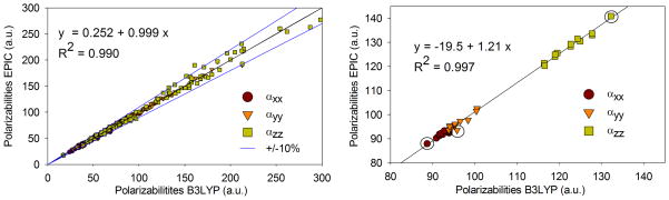
Correlation between B3LYP/aug-cc-pVTZ polarizability components and the EPIC model P2E. In (a), the polarizability components for all sets of Figure 3 are correlated and the ±10% error lines are illustrated. The linear regression shows excellent agreement, especially for polarizabilities smaller than 150 a.u. In (b), 13 stable conformers of n-octane are examined. The all trans conformation polarizabilities are identified with circles. The average polarizability error on the 13 conformers is 1.9% and the anisotropy error is 5.8%. A linear regression gives a R² of 0.997, a slope of 1.21 and an ordinate at the origin of −19.5. This means that the EPIC model P2E overestimates the polarizability of n-octane consistently through all conformers.

The pyridones-v set is the most challenging with the highly functionalized purine derivates (purine, hypoxanthine and uric acid) and the substituted pyridones with five member heteroaromatic rings. For example, the geometry optimized 1-(2-thienyl)-pyridin-4-one shows an angle of 58 degrees between the two aromatic rings as opposed to the 1-(oxadiazol)-imidazolone that has the two connected rings coplanar and a fully delocalized electron π system. This dataset is similar to the chemical functionalization of drug-like molecules.

The average angles between the eigenvectors of the polarizability components of B3LYP and EPIC are less than 5.5 degrees in all sets, although in some molecules the angles can be as large as 23 degrees, i.e. for thiazole. For the pyridones-t and pyridones-v sets, the angular diffences remain surprisingly small.

Finally, Table 4 shows that compared to experimental values, the parameterized EPIC method performs comparably to B3LYP against the subset of 25 molecules for which experimental data is available. Indeed, EPIC produces a δ_avg of 3.9% with experiment compared to 4.1% for B3LYP. It also gives a δ_aniso of 9.0% with experiment compared to 10.5% in the case of B3LYP. The STDEV of the errors from B3LYP match EPIC values. The discrepancy between B3LYP and EPIC calculated for the molecules of Figure 3 is smaller leading to a δ_avg of 1.9% and a δ_aniso of 4.6%. The level of error compared to experiment obtained with both B3LYP and EPIC is not necessarily beyond experimental uncertainty.

Table 4.

Average errors and stdev against experiment^a for all molecules in Figure 3.

Method	δavg (%)	Stdev (%)	δaniso (%)	stdev (%)
Tan et al.b	58.4	19.8	13.6	9.4
Bondic	8.3	6.2	22.4	13.5
EPIC/P2Ed	3.9	4.1	9.0	9.5
EPIC/P1Ed	3.8	3.1	7.3	6.4
B3LYP	4.1	4.1	10.5	9.9

^a25 experimental average polarizabilities and 18 anisotropy data. Details given in Supporting Information.

^bReference 12.

^cBondi radii and ε_in = 4.

^dEPIC used with parameters fit in this work reported in Table 3.

5.5 Conformational dependency of polarizability

Although we avoided comparing the polarizability of flexible molecules to experimental data, it is obvious that a good empirical method should account for the conformational dependency of the polarizability, the anisotropy and the orientation of the polarizability tensor eigenvectors. In addition to the deliberate choice of a wide range of 3D diversity in our molecular sets, we examined the case of n-octane, the most flexible molecule of the sets. Taking 13 diverse B3LYP geometry optimized conformers of n-octane, we computed the polarizability, anisotropy and the eigenvectors using the P2E parameters. The EPIC method gives average polarizability error and anisotropy error of 1.9% and 5.8% respectively. Figure 5b shows a correlation graph between B3LYP polarizability components and our model (α_xx, α_yy, α_zz). The correlation is perfectly linear as shown by a linear regression leading to a R² of 0.997 although the slope of the regression is 1.21, consistent with the average errors outlined above. Moreover, in Figure 5a, we clearly see that correlation of the polarizability components for all the molecules of Figure 3 is excellent with a slope of 1 and a R² of 0.990. This result leads to the conclusion that our model is at least consistently making the same errors for n-octane conformers compared to B3LYP. Finally, the orientations of the polarizability components differ by 0.97 degrees with a maximum value of 3.7 degrees; this is in spite of the broken symmetry in the gauche octane conformers.

6. Discussion

6.1 Transferability

Shanker and Applequist¹⁵, with a variation of the PID model, studied seven nitrogen heterocyclic molecules that we also included in our sets: pyridine, pyrimidine, pyrazine, 9H-purine, quinoxaline, quinoline and phenazine. Using 12 parameters including directional atomic polarizabilities, they show an average polarizability (eqn 10) and anisotropy errors (eqn 9) of 10% and 12% respectively⁶⁶; the parameterized EPIC (Table 3) produces correspondingly 3% and 5% of error with only 4 parameters; we feel that the reduced requirement for fitted parameters is due to a better physical model. Similar comparisons can be made to the work of Miller²¹ where it is reported that 6 parameters for benzene, 9 parameters for pyridine, 9 parameters for naphthalene and 12 parameters for quinoline are needed to obtain both the average polarizability and anisotropy. With the EPIC method, again the same 4 parameters do for all.

Recently, Williams and Stone⁶⁷ have parameterized a polarizable model on n-propane, n-butane, n-pentane and n-hexane in both their trans and gauche conformations. With their simplest Ctg model, they use 10 atomic polarizability parameters to fit the polarizability tensors to B3LYP values. They obtain a very small error on both the average polarizability and the anisotropy of 1.16% and 2.37% respectively. Making the same comparison with our model, we obtain 1.7% of average polarizability error and 3.99% of anisotropy error. Although the error is slightly larger with our EPIC model, this is obtained with only three parameters also producing similar levels of errors in our extended set of alkanes. Furthermore, the level of errors reported by Williams et al. and our studies are all within the accuracy of B3LYP method.

The small number of parameters (c.f. Table 3) needed to fit all the aromatic compounds of Figure 3 is a good indication of the transferability and the generality of the method for heteroaromatic compounds. For example the same nitrogen radius could simultaneously fit pyridine, pyridone, pyrrole, and even branched nitrogen. In the case of alkanes, we have examined most characteristic shapes. Moreover, the training and validation sets produce similar errors, thus the expected performance of our method in the general case can be approximated by the errors on the validation sets.

Overall, we obtain the same level of error as the best PID methods parameterized with anisotropic atomic polarizabilities and about threefold more parameters. Although the number of parameters is not an issue for a small and homogenous set of molecules, it would become a serious barrier for further development of a model applicable to the immense functional group complexity of drug-like molecules, one of the main goals of this ongoing effort.

6.2 Inner dielectrics

The choice of fitting two inner dielectrics, one for the alkanes and one for the heteroaromatics, makes the calculation of new mixed molecules such as t-butylbenzene not possible unless we have a way to switch from a high dielectric (benzene) to a lower dielectric (t-butyl) intramolecularly. Overall, the value of multiple dielectrics, based on chemical constituency, seems proven as well as being physically reasonable. This is a potentially useful strategy in the development of a future general polarizability model. However, simultaneously fitting the polarizabilities of all the compounds from Figure 3 with a single dielectric still gives reasonable results. Table 3 reports the values of the optimal parameters used to produce the data of Figure 4c and d. We fit one radius per element except for oxygen, which is split into furan-like and pyridone-like, and for carbon which is split into alkane and aromatic. We first had two hydrogen radii, but there was no significant cost to merge them into one single radius. The results, shown in Figure 4c and d, when compared with those of Figure 4a and b, show a significant increase in the errors on the alkanes-t and alkanes-v sets although the errors on the heteroaromatics classes remain similarly small. It is nevertheless surprising that the level of error remains low when describing the electronic dielectric with a single constant when, in principle, the electronic local polarization should vary intramolecularly as suggested by Oxtoby⁶⁸.

Finally, it is reassuring that the best radii for both reported parameterizations follow the chemical sense of atomic size. The remarkably reduced size of the optimal radii compared to conventional vdW radii (like Bondi) is worth few comments. First, the EPIC radii explain a different physics than conventional vdW radii: the latter relate to the repulsive forces that keep molecules apart whereas the former relate to the electronic response inside the molecule. There is no reason a priori that they would be the same. Furthermore, the high dielectric and the small radii are necessary to modulate the molecular shape so as to correctly fit the polarizability anisotropy. For example, a benzene molecule is flattened when the carbon radii are reduced and thus the out-of-the-plane polarizable volume is reduced while the in-the-plane length is more or less conserved, increasing the anisotropy. With smaller radii reducing the molecular volume for dielectric response, a higher dielectric value is then needed to conserve the molecular polarizability (c.f. eq. 3).

6.3 Link to the optical dielectric constants

Intramolecular dielectric constants in the context of PE or PB can adopt many values depending on the system and the phenomena involved^35,37,58,69 and have been attributed values from 1 to 20. The optimal inner dielectric of solutes in continuum solvent free energy and in ligand-protein binding calculations do not agree³⁷. Here, we attempt to position our work in this jungle of dielectrics.

We are concerned uniquely with the electronic polarization component. None of the optimal dielectric constants fitted in this work match the experimental optical dielectric constants calculated as the square of the refractive index, which normally have values between 1.2 and 4.0. We partly justify the need for larger dielectrics in section 6.2, but there are other factors that should also be considered. It is important to realize that the link between the molecular polarizability and the macroscopic optical dielectric constant is given by the Lorentz-Lorenz relation shown in eqn 12 where N is the number of molecule in the volume V and ε is the macroscopic dielectric when the light frequency is high compare to the dipolar or ionic relaxation time (ε₀ is the vacuum permittivity constant).

$${\alpha }_{\mathit{avg}}=\frac{3{\epsilon }_{0}V}{N}\left[\frac{\epsilon -1}{\epsilon +2}\right]$$ 12

In the Lorentz-Lorenz equation a molecule is approximated as a spherical dielectric with an effective molecular volume given by the ratio of the macroscopic space occupied by one molecule. However, from our atomistic perspective the effective volume of a molecule is defined by the electronic density and does not include the empty space between molecules effectively included in eqn 12. Hence, in the EPIC model that we parameterize, the average polarizability is the link to refractive index and not the inner dielectric. The main reason for this is the inconsistency between the atomistic and macroscopic definitions of the molecular volume. This raises the point that using experimental optical dielectrics assigned to the solute interior in continuum solvent approaches should be further questioned.

Finally, we believe that a more accurate treatment of solute polarizability in the context of continuum solvent could improve the quality of continuum dielectric methods. Obviously the radii and dielectrics obtained in the present work cannot be used in the condensed phase directly; conventional vdW radii should be used as the basis for intermolecular contacts (such as hydrogen bonding) and the solvent boundary. Therefore, to simultaneously include the solute electronic response and the correct solvent response, there is a dielectric region, which still needs to be characterized, in between our small “polarizability” radii and the vdW radii. Although out-of-scope for the present article, we are in the process of extending the use of our findings in this direction. Once done, one could think of obtaining a polarizable model close to the ‘polarizable continuum model’ (PCM) of Tomasi⁷⁰ in which the electronic density would be simply replaced by an ‘electronic volume’ defined with radii and a dielectric constant.

Conclusion

In this work, the simple physical picture afforded by a continuum dielectric representation has been used to accurately model molecular dipole polarizability tensors. The molecular inner dielectric in the EPIC model accounts for the electronic polarization. To tackle gas-phase polarizabilities, we capitalized on existing finite difference Poisson-Boltzmann code to calculate the induced dipole moment of a molecule in vacuum in the presence of a uniform electric field. As opposed to the usual use of PE or PB in continuum models, the molecule is a region of higher dielectric and the external dielectric is set to the vacuum value. The calculations are fast and resource-sparing, with equivalently good results up to a grid spacing of 0.5 Å, even though a discrete vdW dielectric boundary is used.

This EPIC model of molecular polarizability possesses some important differences with other approximations such as the point inducible dipole, Drude oscillator, and the fluctuating charge models. It is based on a local differential equation solved on a grid, which brings to the same level of complexity the polarizability and coulombic electrostatic components. Importantly, EPIC avoids the polarizability catastrophe found in the other PID-based models. Furthermore, it allows, in principle, for a more detailed response to the electric field than the PID or the FQ models based on the fact that the response emerges from the electric field lines across the molecule surface instead of evaluations only at atomic nuclear positions.

This study involved the parameterization of atomic radii, used in the definition of the vdW dielectric boundary, and the molecular inner dielectric. Previous values of these parameters found in the literature are unacceptably poor at approximating molecular polarizability, especially the anisotropy. We attribute this discrepancy to the fact that previous models simultaneously optimize different kinds of interdependent parameters fitting to a complex energy property instead of focusing on solute polarization. Indeed, the previous purpose of using dielectric continuum was in the context of continuum solvent, often completely neglecting the solute response per se.

To test the newly proposed method, we selected difficult chemical classes: the homonuclear diatomics, a wide variety of heteroaromatics and a diverse set of alkanes. A total of 5 diatomics plus 48 molecules are part of the training sets, subdivided into 6 chemical classes to which we add 45 molecules for validation purposes. In previous models, the polarizabilities of these classes of compounds were correctly calculated only when anisotropic atomic polarizabilities were employed (or auxiliary sites in the case of FQ). Already, with about threefold less parameters than other studies with different models, we have obtained averaged polarizability errors smaller than 5% and averaged anisotropy errors less than 8% considering all sets. The polarizability components calculated with the EPIC/P2E model correlates very well with B3LYP/aug-cc-pVTZ with a R² of 0.990 and a slope of 0.999. The orientations of the polarizability eigenvectors are also well reproduced. The flexibility of the model even allowed the calculation of an accurate anisotropy for F₂ without resorting to auxiliary sites or anisotropic parameters. We also found that the EPIC model was able to consistently calculate the molecular polarizabilities on 13 different conformers of n-octane. Because of the success of parsimonious parameterization of the EPIC model on difficult chemical classes, we believe that the parameterization can be generalized for all organic chemistry with adequate accuracy. In doing this, we found that intra-molecularly varying dielectric constant might be needed to account for the molecular anisotropy.

Overall, this study exemplified that a phenomena as complex as electronic polarization can be accurately modeled with a simple dielectric continuum model. The principal implications of these findings are in the areas of Poisson-Boltzmann methods and in polarizable force field development. However, the level of accuracy obtained might also have impact beyond our initial consideration, for example in the field of spectroscopy.

References

- 1.Lane NF. Rev Mod Phys. 1980;52:29–119. [Google Scholar]
- 2.Kirkwood JG. J Chem Phys. 1937;5:479–491. [Google Scholar]
- 3.Wagnière GH. Linear and Nonlinear Optical Properties of Molecules; VCH; Helvetica Chimica Acta Publishers; Weinheim: 1993. VCH ed. [Google Scholar]
- 4.Maroulis G, Hohm U. Phys Rev A. 2007;76:032504. [Google Scholar]
- 5.Vela A, Gazquez JL. J Am Chem Soc. 1990;112:1490–1492. [Google Scholar]
- 6.Nagle JK. J Am Chem Soc. 1990;112:4741–4747. [Google Scholar]
- 7.Allen TW, Andersen OS, Roux B. Proc Natl Acad Sci U S A. 2004;101:117–122. doi: 10.1073/pnas.2635314100. [DOI] [PMC free article] [PubMed] [Google Scholar]
- 8.Wick CD, Kuo IFW, Mundy CJ, Dang LX. J Chem Theory Comput. 2007;3:2002–2010. doi: 10.1021/ct700098z. [DOI] [PubMed] [Google Scholar]
- 9.Guo H, Gresh N, Roques BP, Salahub DR. J Phys Chem B. 2000;104:9746–9754. [Google Scholar]
- 10.Lipinski CA, Lombardo F, Dominy BW, Feeney PJ. Adv Drug Deliv Rev. 1997;23:3–25. doi: 10.1016/s0169-409x(00)00129-0. [DOI] [PubMed] [Google Scholar]
- 11.Sharp K, Jean-Charles A, Honig B. J Phys Chem. 1992;96:3822–3828. [Google Scholar]
- 12.Tan YH, Luo R. J Chem Phys. 2007;126:094103. doi: 10.1063/1.2436871. [DOI] [PubMed] [Google Scholar]
- 13.Elking D, Darden T, Woods RJ. J Comput Chem. 2007;28:1261–1274. doi: 10.1002/jcc.20574. [DOI] [PMC free article] [PubMed] [Google Scholar]
- 14.van Duijnen PT, Swart M. J Phys Chem A. 1998;102:2399–2407. [Google Scholar]
- 15.Shanker B, Applequist J. J Phys Chem. 1996;100:3879–3881. [Google Scholar]
- 16.Silberstein L. Philos Mag. 1917;33:521–533. [Google Scholar]
- 17.Bode KA, Applequist J. J Phys Chem. 1996;100:17820–17824. [Google Scholar]
- 18.Applequist J. J Phys Chem. 1993;97:6016–6023. [Google Scholar]
- 19.Applequist J, Carl JR, Fung KK. J Am Chem Soc. 1972;94:2952–2960. [Google Scholar]
- 20.Birge RR. J Chem Phys. 1980;72:5312–5319. [Google Scholar]
- 21.Miller KJ. J Am Chem Soc. 1990;112:8543–8551. [Google Scholar]
- 22.Thole BT. Chem Phys. 1981;59:341–350. [Google Scholar]
- 23.Warshel A, Levitt M. J Mol Biol. 1976;103:227–249. doi: 10.1016/0022-2836(76)90311-9. [DOI] [PubMed] [Google Scholar]
- 24.Cieplak P, Kollman PA, Lybrand T. J Chem Phys. 1990;92:6755–6760. [Google Scholar]
- 25.Kaminski GA, Stern HA, Berne BJ, Friesner RA. J Phys Chem A. 2004;108:621–627. [Google Scholar]
- 26.Noskov SY, Lamoureux G, Roux B. J Phys Chem B. 2005;109:6705–6713. doi: 10.1021/jp045438q. [DOI] [PubMed] [Google Scholar]
- 27.Lamoureux G, Roux B. J Chem Phys. 2003;119:3025–3039. [Google Scholar]
- 28.Gasteiger J, Marsili M. Tetrahedron Lett. 1978:3181–3184. [Google Scholar]
- 29.Rick SW, Stuart SJ, Berne BJ. J Chem Phys. 1994;101:6141–6156. [Google Scholar]
- 30.Rappe AK, Goddard WA. J Phys Chem. 1991;95:3358–3363. [Google Scholar]
- 31.Chelli R, Procacci P, Righini R, Califano S. J Chem Phys. 1999;111:8569–8575. [Google Scholar]
- 32.Harder E, Anisimov VM, Whitfield T, MacKerell AD, Roux B. J Phys Chem B. 2007;112:3509–3521. doi: 10.1021/jp709729d. [DOI] [PMC free article] [PubMed] [Google Scholar]
- 33.Honig B, Nicholls A. Science. 1995;268:1144–1149. doi: 10.1126/science.7761829. [DOI] [PubMed] [Google Scholar]
- 34.Roux B, MacKinnon R. Science. 1999;285:100–102. doi: 10.1126/science.285.5424.100. [DOI] [PubMed] [Google Scholar]
- 35.Antosiewicz J, McCammon JA, Gilson MK. J Mol Biol. 1994;238:415–436. doi: 10.1006/jmbi.1994.1301. [DOI] [PubMed] [Google Scholar]
- 36.Simonson T, Archontis G, Karplus M. J Phys Chem B. 1999;103:6142–6156. [Google Scholar]
- 37.Naim M, Bhat S, Rankin KN, Dennis S, Chowdhury SF, Siddiqi I, Drabik P, Sulea T, Bayly CI, Jakalian A, Purisima EO. J Chem Inf Model. 2007;47:122–133. doi: 10.1021/ci600406v. [DOI] [PubMed] [Google Scholar]
- 38.Fogolari F, Brigo A, Molinari H. J Mol Recognit. 2002;15:377–392. doi: 10.1002/jmr.577. [DOI] [PubMed] [Google Scholar]
- 39.David JG. Introduction to Electrodynamics. 3. Prentice-Hall Inc; Upper Saddle River, NJ: 1999. [Google Scholar]
- 40.Nicholls A. The 233rd ACS National Meeting; Chicago, IL. March 25–29; 2007. [Google Scholar]
- 41.Schropp B, Tavan P. J Phys Chem B. 2008;112:6233–6240. doi: 10.1021/jp0757356. [DOI] [PubMed] [Google Scholar]
- 42.Weininger D. J Chem Inf Model. 1990;30:237–243. [Google Scholar]
- 43.Weininger D, Weininger A, Weininger JL. J Chem Inf Model. 1989;29:97–101. [Google Scholar]
- 44.Weininger D. J Chem Inf Model. 1988;28:31–36. [Google Scholar]
- 45.OMEGA, version 2.2.1. Santa Fe, NM, USA: 2007. [Google Scholar]
- 46.Frisch MJ, Trucks GW, Schlegel HB, Scuseria GE, Robb MA, Cheeseman JR, Montgomery JA, Jr, Vreven T, Kudin KN, Burant JC, Millam JM, Iyengar SS, Tomasi J, Barone V, Mennucci B, Cossi M, Scalmani G, Rega N, Petersson GA, Nakatsuji H, Hada M, Ehara M, Toyota K, Fukuda R, Hasegawa J, Ishida M, Nakajima T, Honda Y, Kitao O, Nakai H, Klene M, Li X, Knox JE, Hratchian HP, Cross JB, Bakken V, Adamo C, Jaramillo J, Gomperts R, Stratmann RE, Yazyev O, Austin AJ, Cammi R, Pomelli C, Ochterski JW, Ayala PY, Morokuma K, Voth GA, Salvador P, Dannenberg JJ, Zakrzewski VG, Dapprich S, Daniels AD, Strain MC, Farkas O, Malick DK, Rabuck AD, Raghavachari K, Foresman JB, Ortiz JV, Cui Q, Baboul AG, Clifford S, Cioslowski J, Stefanov BB, Liu G, Liashenko A, Piskorz P, Komaromi I, Martin RL, Fox DJ, Keith T, Al-Laham MA, Peng CY, Nanayakkara A, Challacombe M, Gill PMW, Johnson B, Chen W, Wong MW, Gonzalez C, Pople JA. Gaussian 03, revision C02. Gaussian Inc; Wallingford CT: 2004. [Google Scholar]
- 47.Becke AD. J Chem Phys. 1993;98:5648–5652. [Google Scholar]
- 48.Becke AD. J Chem Phys. 1993;98:1372–1377. [Google Scholar]
- 49.Stephens PJ, Devlin FJ, Chabalowski CF, Frisch MJ. J Phys Chem. 1994;98:11623–11627. [Google Scholar]
- 50.Frisch MJ, Pople JA, Binkley JS. J Chem Phys. 1984;80:3265–3269. [Google Scholar]
- 51.Clark T, Chandrasekhar J, Spitznagel GW, Schleyer PV. J Comput Chem. 1983;4:294–301. [Google Scholar]
- 52.Rice JE, Handy NC. J Chem Phys. 1991;94:4959–4971. [Google Scholar]
- 53.Woon DE, Dunning J. J Chem Phys. 1993;98:1358–1371. [Google Scholar]
- 54.Kendall RA, Dunning J, Harrison RJ. J Chem Phys. 1992;96:6796–6806. [Google Scholar]
- 55.Hammond JR, Kowalski K, deJong WA. J Chem Phys. 2007;127:144105. doi: 10.1063/1.2772853. [DOI] [PubMed] [Google Scholar]
- 56.Grant JA, Pickup BT, Nicholls A. J Comput Chem. 2001;22:608–640. [Google Scholar]
- 57.Kassimi NEB, Lin ZJ. J Phys Chem A. 1998;102:9906–9911. [Google Scholar]
- 58.Rankin KN, Sulea T, Purisima EO. J Comput Chem. 2003;24:954–962. doi: 10.1002/jcc.10261. [DOI] [PubMed] [Google Scholar]
- 59.MacKerell AD, Bashford D, Bellott M, Dunbrack RL, Evanseck JD, Field MJ, Fischer S, Gao J, Guo H, Ha S, Joseph-McCarthy D, Kuchnir L, Kuczera K, Lau FTK, Mattos C, Michnick S, Ngo T, Nguyen DT, Prodhom B, Reiher WE, Roux B, Schlenkrich M, Smith JC, Stote R, Straub J, Watanabe M, Wiorkiewicz-Kuczera J, Yin D, Karplus M. J Phys Chem B. 1998;102:3586–3616. doi: 10.1021/jp973084f. [DOI] [PubMed] [Google Scholar]
- 60.Bondi A. J Phys Chem. 1964;68:441–451. [Google Scholar]
- 61.Sekino H, Maeda Y, Kamiya M, Hirao K. J Chem Phys. 2007;126:014107. doi: 10.1063/1.2428291. [DOI] [PubMed] [Google Scholar]
- 62.van Faassen M, de Boeij PL. J Chem Phys. 2004;120:8353–8363. doi: 10.1063/1.1697372. [DOI] [PubMed] [Google Scholar]
- 63.van Faassen M, Jensen L, Berger JA, de Boeij PL. Chem Phys Lett. 2004;395:274–278. [Google Scholar]
- 64.van Faassen M. Int J Mod Phys B. 2006;20:3419–3463. [Google Scholar]
- 65.Leupin W, Berens SJ, Magde D, Wirz J. J Phys Chem. 1984;88:1376–1379. [Google Scholar]
- 66.For purine and quinoxaline, the B3LYP/aug-cc-pVTZ components from this work are used for the comparison since they match the experimental average polarizability reported by Shanker et al. Averaged experimental components reported by Shanker et al. are used for pyrimidine and pyrazine.
- 67.Williams GJ, Stone AJ. Mol Phys. 2004;102:985–991. [Google Scholar]
- 68.Oxtoby DW. J Chem Phys. 1980;72:5171–5176. [Google Scholar]
- 69.Elcock AH, Sept D, McCammon JA. J Phys Chem B. 2001;105:1504–1518. [Google Scholar]
- 70.Miertus S, Scrocco E, Tomasi J. Chem Phys. 1981;55:117–129. [Google Scholar]
- 71.Rowland RS, Taylor R. J Phys Chem. 1996;100:7384–7391. [Google Scholar]