A PROGRESSIVE RUPTURE MODEL OF SOFT TISSUE STRESS RELAXATION

Abstract

A striking feature of stress relaxation in biological soft tissue is that it frequently follows a power law in time with an exponent that is independent of strain even when the elastic properties of the tissue are highly nonlinear. This kind of behavior is an example of quasi-linear viscoelasticity, and is usually modeled in a purely empirical fashion. The goal of the present study was to account for quasi-linear viscoelasticity in mechanistic terms based on our previously developed hypothesis that it arises as a result of isolated micro-yield events occurring in sequence throughout the tissue, each event passing the stress it was sustaining on to other regions of the tissue until they themselves yield. We modeled stress relaxation computationally in a collection of stress-bearing elements. Each element experiences a stochastic sequence of either increases in elastic equilibrium length or decreases in stiffness according to the stress imposed upon it. This successfully predicts quasi-linear viscoelastic behavior, and in addition predicts power-law stress relaxation that proceeds at the same slow rate as observed in real biological soft tissue.

Introduction

Biological soft tissues of all kinds are highly viscoelastic, which means that they exhibit a transient relaxation in stress following sudden stretch to a new fixed length.^{7, 13, 14} A striking feature of stress relaxation in these materials is that its time course frequently follows a power law such that stress (σ) decays with time (t) according to

$$\sigma (t)=a(\epsilon )t^{-k}$$ (1)

where a(ε) is a (usually nonlinear) function of the strain (ε) imposed on the tissue. In lung parenchymal tissue, for example, k is a positive constant much less than unity that is virtually independent of ε.⁷ The equivalent behavior in the frequency domain is a complex modulus that varies linearly with frequency, which has been reported in biological soft tissue such as lung parenchyma⁷ as well as individual cells¹² and even biopolymer gels.⁹

What is most intriguing about Eq. 1, however, is that the static nonlinear stress-strain behavior embodied in the function a(ε) is separable from the dynamic behavior represented by t^−k. This phenomenon of separability is an example of quasi-linear viscoelasticity, a phenomenon first described by Fung.¹³ Quasi-linear viscoelasticity is not found in all soft tissues, e.g.²³, but it has been reported to occur in a wide variety that includes lung^{7, 22}, heart valve¹⁰, ligament¹⁴, muscle^{23, 32}, and plantar tissue.²⁵ Despite the widespread appearance of quasi-linear viscoelasticity, however, understanding its mechanistic basis has remained a challenge.

We recently described a model of soft tissue that may capture some of the mechanistic essence of quasi-linear viscoelasticity.⁴ The model consists of a collection of spring-and-dashpot pairs (Maxwell bodies) whose springs are recruited to bear stress in a sequential fashion when the dashpots in other Maxwell bodies reach the end of their travel and fall apart. We showed analytically that stress in this model relaxes asymptotically in time according to a power law. Further, the value of k in Eq. 1 for this model is determined only by the nonlinear constitutive properties of its springs and dashpots, and is therefore independent of strain. The quasi-linear viscoelastic behavior of this model is attributable to the sequential nature of the role played by each of its comprising Maxwell bodies, and the fact that each body must disintegrate before the next comes into play.⁴ The behavior of these Maxwell bodies is not compatible with stress relaxation occurring through the simultaneous movement of many fibers sliding smoothly past each other, as is usually conceived. Instead, the implication is that stress is relieved through a series of isolated micro-yield events occurring in sequence throughout the tissue, each event passing the stress it was sustaining on to other regions of the tissue until they themselves yield.

This raises the question as to what these micro-yield events might actually correspond to in real tissue. Presumably such events represent the breaking of discrete junctions between structural elements, and in fact there is precedent for this in the literature. Mijailovich et al.²⁰ developed a computational model in which the mechanical integrity of soft tissue was maintained through temporary contact junctions between elastic protein fibers in intimate apposition. When longitudinal stress exceeded the yield strength of the bonds the fibers moved laterally with respect to each other, leading to the prediction of qualitative behavior reminiscent of experimental observation. More recently, Donovan et al.¹¹ proposed that soft tissue rheology reflects the breaking of fiber-fiber interactions mediated by cross-linker proteins extending from one fiber and attaching to electrostatic binding sites on an adjacent fiber. Again, these investigators were able to recapitulate key features of experimental data, including so-called fluidization that manifests as a transient decrease in tissue stiffness following sudden brief stretch.^{11, 29} Although the stress relaxation behavior predicted by these previous models differed from a power law, these studies nevertheless suggest that the essence of tissue stress adaptation is the probabilistic breaking and reforming of temporary bonds between structural fibers according to the stress borne by the bonds. Accordingly, the goal of the present study was to explore the extent to which this general mechanism, independent of any particular anatomic realization, can account for the key features of quasi-linear power-law stress relaxation.

Computational Methods and Results

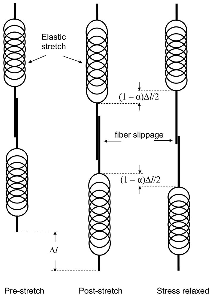
We consider the fundamental stress-bearing element in biological soft tissue to be a pair of elastic fibers oriented in the direction of tissue strain and connected to each other by a temporary bond. The bond is formed by inter-molecular forces of some kind, but the precise details are unimportant for the purposes of the model. What is important is that when the fibers are pulled in opposite directions they elongate until the force between them causes the bond to break. When this happens, the two fibers retract elastically in opposite directions until the tension between them falls to a point where another temporary bond can form, as illustrated in Fig. 1. We assume that the breaking and reforming of bonds are stochastic processes that happen with probabilities that depend on the stresses applied to the bonds, similar to the behavior of cross-linkers between protein fibers as modeled by Donovan et al.¹¹

Figure 1.

The basic 3-step stress relaxation mechanism in the computational model. Left: a pair of relaxed elastic fibers joined by a temporary bond. Middle: the fibers strained by an amount Δl with bond between them intact. Right: the fibers after the bond between them has failed and then reformed at reduced stress, thereby increasing the combined relaxed length of the pair by (1 − α)Δl.

Using a model coded in Visual Basic (Microsoft), we first investigated the stress relaxation behavior of a model consisting of a parallel collection of 200 identical fiber pairs. Simulations were performed beginning with the fibers being stretched by an amount Δl₀ beyond their common elastic equilibrium length. This generated an initial total elastic force, F₀, given by the sum of the identical forces across all fiber pairs thus:

$$F_0=\sum _{j=1}^{200}E{\left(\mathrm{\Delta }{l}_0\right)}^q$$ (2)

where E is an elastic constant and q is an exponent determining the degree of elastic nonlinearity. (As most soft tissues exhibit strain stiffening, we would generally expect q to be greater than 1.)

To calculate the relaxation in force across the model at the first time step in the simulation, we implemented the slip process described above in a probabilistic manner that scaled with force as follows. For each fiber pair in turn, we drew a value x from a uniform distribution on the interval (0, 1) and allowed the pair to slip if the condition

$$x<P_{\mathit{slip}}{f}_j$$ (3)

was satisfied, where P_slip is a constant determining the slip probability for all fibers and f_j is the force in the j^th fiber pair. Bonds were thus broken between only a fraction of the 200 fiber pairs, allowing the two members of these pairs to retract elastically by having their overlapping ends slip past each other to allow a new bond to form at a lower level of stress (as illustrated in Fig. 1). Those fiber pairs that slipped in this manner experienced an increase in their combined elastic equilibrium lengths such that their new extensions beyond this length became αΔl₀, where 0 < α < 1. The extensions of the remaining non-slipped fibers remained at Δl₀. In other words, in calculating the total force, F₁, across the model at the end of the first time step, Eq. 2 must be modified to take the individual extensions of the fiber pairs into account thus:

$$\begin{array}{l}{F}_1=\sum _{j=1}^{200}{f}_{j,1}\\ =\sum _{j=1}^{200}E{\left(\mathrm{\Delta }{l}_{j,1}\right)}^q\end{array}$$ (4)

where f_j,1 is the force across the j^th fiber pair and Δl_j,1 is its extension at the end of time step 1. Equation 4 was used to calculate F_n for all subsequent time steps according to the probabilistic slip process embodied in Eq. 3. That is

$$\begin{array}{lll}\mathrm{\Delta }{l}_{j,n}\hfill & =\mathrm{\Delta }{l}_{j,n-1}\hfill & ifx\ge P_{\mathit{slip}}{f}_{j,n-1}\hfill \\ \hfill & =\alpha \mathrm{\Delta }{l}_{j,n-1}\hfill & ifx<P_{\mathit{slip}}{f}_{j,n-1}\hfill \end{array}$$ (5)

Model simulations were run for 10,000 time steps.

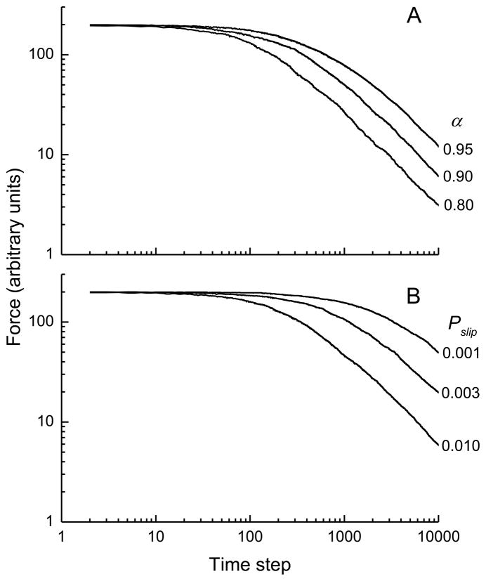
Figure 2A shows a log-log plot of the time course of force across the model with E = 1, P_slip = 0.01, and q = 3 following a step strain of 1 when α had values of 0.95, 0.90 and 0.80. The figure shows that increasing the mean amount by which each fiber slips whenever there is a yield event (governed by the parameter α) causes a decrease in the duration of the initial stress transient, but the asymptotic relaxation rate in each case is governed by a power law with a value of k very close to 1. Figure 2B shows similar results when the value of α is fixed at 0.9 and the probability that a yield event will occur (P_slip) takes values of 0.01, 0.003 and 0.001. Here, again, the asymptotic slope of the log(force)-log(time) plot is −1, with a greater probability of fiber slippage resulting in a shorter initial transient phase.

Figure 2.

Simulations of stress versus time from the computational model in which A) the average amount of slip per yield event was varied (governed by the parameter α) as shown, and B) the probability that a stressed bond would fail was varied (governed by the parameter P_slip) as shown. See text for the remainder of the model parameter values and initial conditions.

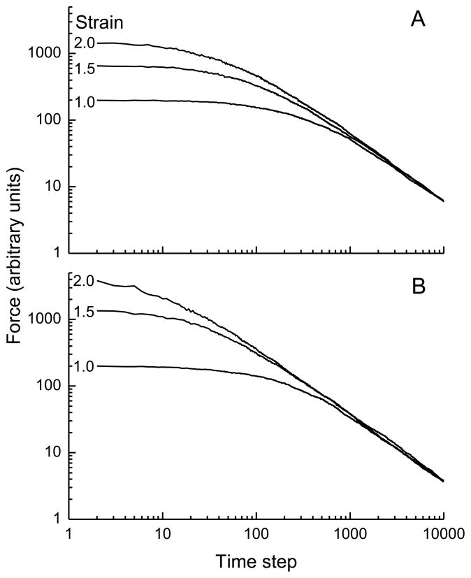
Figure 3 shows that the model produces the same asymptotic slope in force when the initial step change in strain is varied in the presence of different degrees of spring nonlinearity; Fig. 3A illustrates this behavior for strains of 1.0, 1.5 and 2.0 (i.e. extensions of 100%, 150% and 200% above baseline) when the springs have a cubic dependence of force on strain, while in Fig. 3B spring force depends on strain raised to the fifth power. (Note that these strains may be larger than those usually encountered physiologically in many biological tissues, but our purpose here is to examine the universality of behavior rather than relate it to normal function. In any case, the qualitative behavior of the model is independent of strain.) The remaining model parameters in Fig. 3 are E_j = 1, α = 0.9, and P_slip = 0.01. Figure 3 thus demonstrates that the model exhibits behavior reflective of quasi-linear viscoelasticity. However, the asymptotic slopes in Fig. 3 are approximately −1 and the linear parts of the relationships all superimpose. Both of these features are at variance with experimental data showing force-time relationships that are displaced vertically with increasing strain, and with slopes that are much smaller than those see in Figs. 2 and 3. For example, in strips of degassed lung parenchyma the value of k has been reported to be an order of magnitude smaller than the values of 1 seen in Figs. 2 and 3.⁷ The same is true for the lung as a whole; the frequency-domain equivalent of power-law stress relaxation with a small value of k is a constant-phase mechanical impedance in which the real and imaginary parts decrease in magnitude with the inverse of frequency raised to a power close to unity ⁸, and whole intact lungs behave precisely in this manner.¹⁶

Figure 3.

Simulations of stress versus time in which the magnitude of the initial step change in model strain was varied as shown. A) shows results obtained when the stress in each elastic fiber in the model depends on its extension raised to the third power, while B) shows correspond results when stress depends on strain raised to the fifth power. See text for the remainder of the model parameter values and initial conditions.

It would therefore seem that our computational model requires the incorporation of a mechanism to progressively reduce the amount of slippage between its fiber pairs so that the resulting relaxation of stress slows down accordingly. One possible way of achieving this is suggested by the notion that the mechanical yield events occurring within a sample of stressed soft tissue are likely to manifest over a wide range of length scale. We have so far modeled these yield events as occurring between individual fibers of the same size. In reality, it seems more likely that large contiguous collections of fibers might maintain some degree of structural integrity, at least initially following stretch, so that early yield events represent the slippage of one large collection relative to another. As time proceeds, however, sub-collections of fibers within each large collection may start to slip with respect to each other, and then sub-sub-collections within each sub-collection, and so on down to ever smaller scales. In other words, we propose that slippage events continue to occur within each of the initial large fiber collections, but the slippage magnitudes become progressively smaller with time.

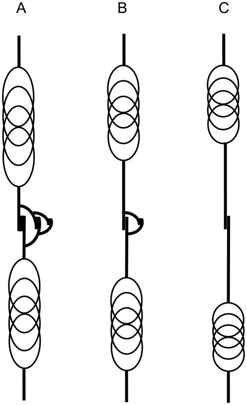
In developing the above model, we stipulated that a broken slip bond between two fibers reforms when the stress between the fibers has fallen to some lower level, but now we need to give some thought as to how this could actually happen. If the bond between the two fibers behaves like static friction, then once the bond fails it is likely that it will not reform again until the two fibers have essentially ceased to move with respect to each other. At this point the stress between them would have fallen to zero, which is not likely to lead to a slow rate of stress relaxation within the tissue as a whole. On the other hand, real tissue is composed of fibers that are aligned in all directions, including some that are perpendicular to the direction of strain and which would presumably be relatively slack even when the more aligned fibers are under tension. This allows for the possibility that these slack fibers might suddenly come under tension if they span a slip bond that fails. A simple representation of this mechanism is shown in Fig. 4 which shows a pair of elastic fibers joined by a slip bond as before (Fig. 1A), but now there exists an additional pair of smaller fibers connected to the first pair either side of the slip bond. Before the bond breaks these secondary fibers are flaccid, but when the bond breaks they become straightened so that their own slip bond comes under tension. When this bond breaks an even smaller set pair of fibers is recruited, and so on. In this way, the elastic equilibrium length of the whole assembly becomes progressively longer, but in ever decreasing increments. Figures 4B and 4C illustrate this concept.

Figure 4.

Schematic representation of fiber slippage occurring over multiple length scales. When the first slip occurs the retraction of the fibers is halted temporarily by the straightening of a second pair of fibers. When the bond between this second fiber pair fails a third shorter pair come into play, and so on. The relaxed length of the entire assembly thus increases over time by ever decreasing increments.

To mimic the scale-dependent mechanism described above, we made the amount of slip between each fiber pair in the computational model depend inversely on the number of prior slips between that pair. That is, Eq. 5 was modified to be

$$\begin{array}{lll}\mathrm{\Delta }{l}_{j,n}\hfill & =\mathrm{\Delta }{l}_{j,n-1}\hfill & ifx\ge P_{\mathit{slip}}{f}_{j,n-1}\hfill \\ \hfill & =\frac{\alpha }{n_j}\mathrm{\Delta }{l}_{j,n-1}\hfill & ifx<P_{\mathit{slip}}{f}_{j,n-1}\hfill \end{array}$$ (6)

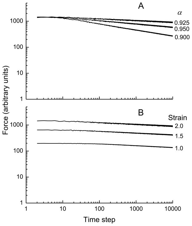
where n_j is the number of prior slips in the j^th fiber pair (n_j = 1 for the first time step). With this addition, we find that the slope of the force-time relationship (i.e. the value of k) can be tuned through the choice of α as shown in Fig. 5A. For example, by setting α = 0.95 we achieved a value of k = 0.07, which is close to experimentally observed values.⁷ This contrasts significantly with the previous version of the model, based on Eq. 3, in which α had no influence on k (Fig. 2A). Figure 5B shows that the revised model, based on Eq. 6, gives a value of k that is independent of strain as before, but now the relationships separate vertically with strain, thereby demonstrating behavior highly reminiscent of the quasi-linear viscoelastic behavior we have observed previously in strips of lung tissue.⁷

Figure 5.

Simulations of stress versus time when the multi-scale slip mechanism illustrated in Fig. 4 is incorporated. A) shows results for different average magnitudes of slip per yield event (governed by the parameter α), while B) shows results for different initial strains. See text for the remainder of the model parameter values and initial conditions.

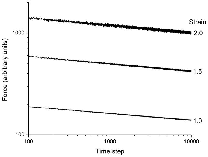
To test the robustness of the model, we simulated stress relaxation following strains of 1, 1.5, and 2 (i.e. fractional increases in length above baseline) when α for each fiber pair was assigned a value chosen randomly with equal probability between the limits of 0.95 and 1.00, q was chosen randomly from between 1 and 5, and E was chosen randomly from between 1 and 5. In addition, to incorporate the realism of having fibers arranged in both series and parallel, we extended the model so that it comprised 4 units connected end to end, with each unit consisting of 200 fiber pairs. At each time step, the amounts of stretch in the fiber pairs were iteratively adjusted until the forces across all units were identical, while equal lengths were maintained for each fiber pair in a given unit. This was achieved by changing all fiber pair lengths in a given unit by a small amount in the direction of the mean force across the unit until the maximum difference in force across all units fell below 0.1% of the average force. The average force then provided the stress relaxation time course for the model. Figure 6 shows the later linear portions of the resulting force-time relationships in a log-log plot. These relationships separate vertically and all have a slope of about −0.07, and are thus very similar to our previously reported values of k from strips of lung tissue.⁷

Figure 6.

Stress versus time in the computational model following different initial step strains when the parameters of the model were chosen randomly from various probability distribution functions (see text for details), demonstrating the robustness of the model to variations in its parameters values.

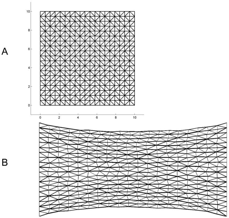
Finally, to test the robustness of the micro-yield mechanism of stress relaxation to variations in fiber direction, we incorporated it into a two-dimensional elastic network implemented in Matlab (Mathworks, Natick, MA). Here we invoked a different micro-yield mechanism to that used above. Specifically, we imagine each link in the 2-dimensional network to be composed of numerous elastic filaments in parallel. Damage to a fiber manifests as the rupture of one or more of its filaments, whereupon the overall stiffness of the element suddenly decreases in proportion to the number of ruptured filaments. Thus, rather than representing a micro-yield event as an increase in the elastic equilibrium length of the element as in Eqs. 5 and 6, here we represent it as a decrease in elastic modulus of the element. Figure 7A shows the unstressed configuration of the network, with each element at its elastic equilibrium length. Upon extension, the force, F, in an element is given by

Figure 7.

Two-dimensional network of elastic elements showing A) its relaxed configuration, and B) immediately after a horizontal strain of 1. The thickness of the lines in the strained image indicates the relative force in each element.

$$F=ux+{vx}^2$$ (7)

where u = 1 and v = 10 and x is the extension of an element beyond is equilibrium length in the same arbitrary length units as used to draw Fig. 7A. Figure 7B shows the configuration of the network immediately following a strain of 1, determined using a finite element approach as previously described.³¹ We then relaxed the network, with strain fixed at 1, for 1000 time steps by applying Eq. 3 with P_slip = 0.5 to each element at each time step. However, instead of using Eq. 6 to implemented relaxation, we progressively decreased the elastic constants in Eq. 7 according to

$$\begin{array}{lll}{u}_{j,n},v_{j,n}\hfill & =u_{j,n-1},v_{j,n-1}\hfill & ifx\ge P_{\mathit{slip}}{f}_{j,n-1}\hfill \\ \hfill & =\left(1-\frac{\beta }{n_j}\right)u_{j,n-1},\left(1-\frac{\beta }{n_j}\right)v_{j,n-1}\hfill & ifx<P_{\mathit{slip}}{f}_{j,n-1}\hfill \end{array}$$ (8)

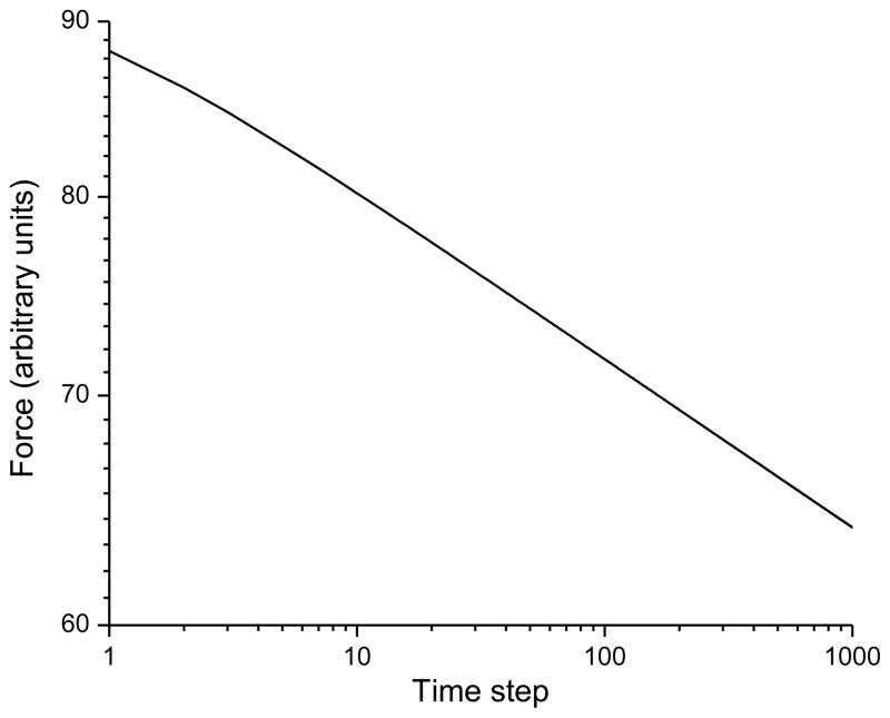
with β = 0.05. Figure 7C shows the configuration of the network after 1,000 time steps. Figure 8 shows that the force across the network as a function of time exhibits the same kind of initial transient as exhibited by the fiber-pair models above, and then becomes log-log linear after about 100 time steps, this time with a slope of −0.05.

Figure 8.

Stress versus time following a strain of 1 in the network shown in Fig. 7. The scale shows the arbitrary length units used in the model.

Discussion

Quasi-linear viscoelasticity has been widely invoked to account for the complex rheological behavior observed in biological soft tissues, but is usually modeled in a purely empirical fashion^{24, 25, 32}. Accounting for the phenomenon in mechanistic terms has been a challenge. Conventional spring-and-dashpot models can be made to mimic quasi-linear viscoelasticity, but only if each spring and its associated dashpot both exhibit identical constitutive nonlinearities^{6, 24}. In this way, the two elements together manifest a fixed time constant, but what this might represent physically is unclear. Lanir¹⁷ developed a model of quasi-linear viscoelasticity based on the progressive recruitment of linearly viscoelastic fibers having a particular distribution of unstressed lengths below which they were flaccid, but this mechanism is arguably too specific to account for such a general phenomenon. We previously modeled the phenomenon on the basis of the relative movement of a collection of randomly oriented fibers and found that while the static and dynamic behaviors exhibited by the model appear to be separable, the predictions of both behaviors are qualitatively quite different from experimental observation.³ These various prior attempts to model quasi-linear viscoelasticity in mechanistic terms thus all have significant limitations. By contrast, our recent model,⁴ which is based on the sequential recruitment of springs to share the strain, exhibits both power-law stress relaxation and complete separation of static nonlinear and dynamic linear behaviors without requiring that the constitutive properties of its components adhere to special distribution functions. This model leads to the notion that stress is gradually relieved in strained biological soft tissue as a result of the sudden structural yielding of local points of high stress, causing stress to be increased in other regions that then eventually yield themselves. In this way, the burden of bearing stress is passed around from one region of the tissue to another.

The purpose of the present study was to incorporate the essence of our previous analytical model⁴ into a model that better resembles actual tissue from a structural point of view. Thus, rather than employing a sequence of springs with disengaging dashpots,⁴ first we represented the tissue as a collection of pairs of elastic fibers, arranged both in series and parallel, that connect to each other via temporary bonds allowing for stochastic slippage under stress. We purposefully make no attempt to assign particular identities to its constituent fibers or to the mechanisms that link them together through temporary bonds. Because power-law stress relaxation in soft tissue is so ubiquitous, the mechanism responsible for this behavior must be independent of the particular players involved or the precise details of their interactions. Accordingly, our model is based solely around the nonspecific notions that the principle stress bearing elements in biological soft tissue are protein-based fibers, and that relative movement of these fibers under stress occurs as a result of the sudden failure of bonds between them as has been suggested in previous studies.^{11, 20} Our results show that these simple ideas alone lead to predictions of asymptotic power-law stress relaxation that are robust in the face of random variations in the various model parameters (Figs. 2 and 5). Furthermore, the exponent of the power law, k, remains unchanged regardless of the size of the step strain to which the model is subjected (Figs. 3 and 5).

Our 2-dimensional spring network model also shows that power-law stress relaxation is still predicted in the face of variations in fiber orientation (Figs. 7 and 8), as must be the case if the distributed micro-yield mechanism is to apply to real tissues. Even more importantly, our network model result show that mechanism by which stress is relaxed does not have to limited to an increase in fiber equilibrium length; the same qualitative results are obtained if the fibers experience progressive decreases in their stiffness instead (Figs. 1–6 vs. Figs. 7 and 8). In fact, one can imagine a variety of other ways for achieving the release of local stress, such as extrusion of fluid through pores or fiber meshes as is known to happen in some soft tissues.¹⁸ If fluid movement takes place on a local scale over timescales that are short compared to the duration of stress relaxation, this could result in the transmission of local stress from one region of the tissue to another. Even the classic Rouse viscoelastic theory²¹ based on the relative movement of worm-like chains, known as reptation, would seem to fit within the current framework if one considers that reptation on a local scale could correspond to a local yield event. It should also be pointed out that if a collection of parallel fibers either increases its relaxation length or decreases its stiffness, the result under constant stress would be an increase in the length of the entire collection. In other words, these micro-yield events also lead to the prediction of creep. The distributed stochastic micro-yield mechanism is thus very non-specific, matching the ubiquity of the phenomenon we are attempting to account for.

Power law processes seem to abound in nature for reasons that remain controversial, but which have nevertheless given rise to numerous theories. Many of these processes and their associated models are characterized by power law exponents (i.e. k in Eq. 1) that have values in the order of unity.^{1, 2, 26, 28, 30} It was thus not a particular surprise that we found k to be close to 1 in our initial attempts to make a yielding fiber model of stress relaxation (Figs. 2 and 3). The reason for this finding is readily understood, as follows. Although the dynamics of the mechanism illustrated in Fig. 1 are stochastic and spatially distributed, stress relaxing events occur at an average rate that is proportional to stress. Furthermore, the amount of stress that is relieved by these yield events is also proportional to stress, so together these two factors cause stress to be relieved at a rate proportional to the square of stress when averaged over the model. This suggests a differential equation of motion for model stress, F(t), of the form

$$\frac{dF}{dt}=-{AF}^2(t)$$ (6)

where A is a constant. The solution to Eq. 6 is that F(t) is proportional to 1/t, leading directly to the slope of −1 when the log of F(t) is plotted against the log of t. The slope can be reduced further, of course, by raising F(t) to a higher power than 2 in the right-hand side of Eq. 6, but there does not seem to be a compelling physical reason for doing this, and in any case the exponent would have to be disconcertingly large if k is to approach the kinds of values (roughly 0.1) seen experimentally in relaxing strips of tissue ⁷ and in its frequency-domain equivalent of a constant-phase mechanical impedance for whole lungs^{15, 16} and cells.^{12, 29}

There must, therefore, be some other mechanism behind the appearance of low values of k in biological soft tissue. In our previous study,⁴ we achieved low values of k by choosing high degrees of nonlinearity for the elastic and dissipative constitutive properties of the springs and dashpots that are recruited sequentially into the stress bearing role. One might argue, however, that this is a bit contrived because it requires nonlinear behavior of a particular functional form. In the present study, we identified a different mechanism for achieving low values for k, namely by having yield events within the tissue take place on progressively smaller length scales as stress relaxation proceeds. This mechanism is stylized in Fig. 4, and implies that tissue mechanics are determined in a fundamental way by the structural hierarchy of the tissue. Experimental support for this theory remains pending, although there is no particular reason at this point to doubt its plausibility. In any case, by having the mean slippage magnitude between two fibers depend on the number of previous times (n_j) the two fibers have slipped, we gain complete control of the predicted value of k through the parameter α in Eq. 6 or β in Eq. 8. This is interesting because without the functional dependence on n_j, as in Eq. 3, α has no influence on k. The inclusion of the mechanism inherent in Eq. 6 thus suggests that the time-scale independence of stress relaxation, as represented by power-law stress relaxation, is intimately linked to the length-scale independence of the yield events within the tissue that represent the mechanism by which stress is relaxed. This is reminiscent of the work by Schiessel and Blumen²⁷ who employed fractal networks of Maxwell bodies to model power-law mechanical behavior in gels, thereby also making a specific link between scale-free structure and function.

Despite the success of our model in accounting for the nature of stress relaxation, we have yet to extend it to deal with the converse phenomenon, namely stress recovery. When soft tissue strain is suddenly decreased after a period of time under tension, the stress across it decreases equally suddenly, but then immediately starts to increase again in a progressive manner that appears to asymptote toward some intermediate value.^{5, 6} Accounting for stress recovery is also necessary when dealing with the oscillatory behavior of soft tissue, which that often exhibits a power-law dependence of modulus on frequency.^{16, 19, 29} This is the frequency domain counterpart to power-law stress relaxation in the time domain.⁸ The potentially problematic issue here is that the breakage of bonds under tensile stress, as modeled in Fig. 1, results in a plastic deformation that persists after the stress is released. There is some sense in which this behavior is mirrored in nature; strips of both active and passive airway smooth muscle tissue appear to lose much of their ability to maintain stress for extended periods of time following sudden release of a sustained stretch, and it is not always clear that the original stress would ever be regained given the slow rates of recovery that have been observed.⁶ Strips of diaphragm tissue have also been shown to exhibit signs of plastic deformation under stress.²³ On the other hand, the tissues of our body maintain their integrity for years without succumbing to irreversible creep, so there must be some mechanism that eventually restores them to their initial configurations following excursions in strain. One possibility may be that thermal agitation, or some active metabolic process, provides the energy required to eventually replace the energy to the tissue fibers that was lost through the stress-based breakage of fiber-fiber bonds under stress. Another possibility, modeled by Mijailovich et al.,²⁰ is that tissue restoration requires external manipulation as occurs when tissue strips are preconditioned in the laboratory. In any case, this remains an open question.

In conclusion, we have developed a computational model of soft tissue that accurately accounts for quasi-linear viscoelastic power law stress relaxation. The model is based solely on the general mechanism of stochastic micro-yield events within structural elements occurring according to the stress the elements bear and the number of prior events they have experienced. Consequently, the model is applicable to any tissue in which these types of phenomena occur regardless of the particular players involved.

References

- 1.Bak P, Tang C, Wiesenfeld K. Self-organized criticality: An explanation of the 1/f noise. Phys Rev Lett. 1987;59:381–384. doi: 10.1103/PhysRevLett.59.381. [DOI] [PubMed] [Google Scholar]
- 2.Barabasi AL, Albert R. Emergence of scaling in random networks. Science. 1999;286:509–512. doi: 10.1126/science.286.5439.509. [DOI] [PubMed] [Google Scholar]
- 3.Bates JH. A micromechanical model of lung tissue rheology. Ann Biomed Eng. 1998;26:679–687. doi: 10.1114/1.42. [DOI] [PubMed] [Google Scholar]
- 4.Bates JH. A recruitment model of quasi-linear power-law stress adaptation in lung tissue. Ann Biomed Eng. 2007;35:1165–1174. doi: 10.1007/s10439-007-9291-0. [DOI] [PubMed] [Google Scholar]
- 5.Bates JH, Brown KA, Kochi T. Respiratory mechanics in the normal dog determined by expiratory flow interruption. J Appl Physiol. 1989;67:2276–2285. doi: 10.1152/jappl.1989.67.6.2276. [DOI] [PubMed] [Google Scholar]
- 6.Bates JH, Bullimore SR, Politi AZ, Sneyd J, Anafi RC, Lauzon AM. Transient oscillatory force-length behavior of activated airway smooth muscle. Am J Physiol Lung Cell Mol Physiol. 2009;297:L362–372. doi: 10.1152/ajplung.00095.2009. [DOI] [PMC free article] [PubMed] [Google Scholar]
- 7.Bates JH, Maksym GN, Navajas D, Suki B. Lung tissue rheology and 1/f noise. Ann Biomed Eng. 1994;22:674–681. doi: 10.1007/BF02368292. [DOI] [PubMed] [Google Scholar]
- 8.Bates JHT. Lung mechanics. An inverse modeling approach. Cambridge: Cambridge University Press; 2009. [Google Scholar]
- 9.Broedersz CP, Kasza KE, Jawerth LM, Munster S, Weitz DA, MacKintosh FC. Measurement of nonlinera rheology of cross-linked biopolymer gels. Soft Matter. 2010;6:4120–4127. [Google Scholar]
- 10.Doehring TC, Carew EO, Vesely I. The effect of strain rate on the viscoelastic response of aortic valve tissue: a direct-fit approach. Ann Biomed Eng. 2004;32:223–232. doi: 10.1023/b:abme.0000012742.01261.b0. [DOI] [PubMed] [Google Scholar]
- 11.Donovan GM, Bullimore SR, Elvin AJ, Tawhai MH, Bates JH, Lauzon AM, Sneyd J. A continuous-binding cross-linker model for passive airway smooth muscle. Biophys J. 2010;99:3164–3171. doi: 10.1016/j.bpj.2010.09.031. [DOI] [PMC free article] [PubMed] [Google Scholar]
- 12.Fabry B, Maksym GN, Butler JP, Glogauer M, Navajas D, Fredberg JJ. Scaling the microrheology of living cells. Phys Rev Lett. 2001;87:148102. doi: 10.1103/PhysRevLett.87.148102. [DOI] [PubMed] [Google Scholar]
- 13.Fung YC. Biomechanics. Mechanical Properties of Living Tissues. New York: Springer-Verlag; 1981. [Google Scholar]
- 14.Funk JR, Hall GW, Crandall JR, Pilkey WD. Linear and quasi-linear viscoelastic characterization of ankle ligaments. J Biomech Eng. 2000;122:15–22. doi: 10.1115/1.429623. [DOI] [PubMed] [Google Scholar]
- 15.Fust A, Bates JH, Ludwig MS. Mechanical properties of mouse distal lung: in vivo versus in vitro comparison. Respir Physiol Neurobiol. 2004;143:77–86. doi: 10.1016/j.resp.2004.07.012. [DOI] [PubMed] [Google Scholar]
- 16.Hantos Z, Daroczy B, Suki B, Nagy S, Fredberg JJ. Input impedance and peripheral inhomogeneity of dog lungs. J Appl Physiol. 1992;72:168–178. doi: 10.1152/jappl.1992.72.1.168. [DOI] [PubMed] [Google Scholar]
- 17.Lanir Y. On the structural origin of the quaslinear viscoelasrtic behavior of tissue. In: Schmid-Schonbein EW, Woo SLY, Zweisach BW, editors. Frontier in biomechanics. New-York: Springer; 1986. pp. 130–136. [Google Scholar]
- 18.Lu XL, V, Mow C. Biomechanics of articular cartilage and determination of material properties. Med Sci Sports Exerc. 2008;40:193–199. doi: 10.1249/mss.0b013e31815cb1fc. [DOI] [PubMed] [Google Scholar]
- 19.Maksym GN, Kearney RE, Bates JH. Nonparametric block-structured modeling of lung tissue strip mechanics. Ann Biomed Eng. 1998;26:242–252. doi: 10.1114/1.119. [DOI] [PubMed] [Google Scholar]
- 20.Mijailovich SM, Stamenovic D, Fredberg JJ. Toward a kinetic theory of connective tissue micromechanics. J Appl Physiol. 1993;74:665–681. doi: 10.1152/jappl.1993.74.2.665. [DOI] [PubMed] [Google Scholar]
- 21.Mohan A, Doyle PS. Unraveling of a Tethered Polymer Chain in Uniform Solvent Flow. Macromolecules. 2007;40:4301–4312. [Google Scholar]
- 22.Navajas D, Maksym GN, Bates JH. Dynamic viscoelastic nonlinearity of lung parenchymal tissue. J Appl Physiol. 1995;79:348–356. doi: 10.1152/jappl.1995.79.1.348. [DOI] [PubMed] [Google Scholar]
- 23.Navajas D, Mijailovich S, Glass GM, Stamenovic D, Fredberg JJ. Dynamic response of the isolated passive rat diaphragm strip. J Appl Physiol. 1992;73:2681–2692. doi: 10.1152/jappl.1992.73.6.2681. [DOI] [PubMed] [Google Scholar]
- 24.Nekouzadeh A, Pryse KM, Elson EL, Genin GM. A simplified approach to quasi-linear viscoelastic modeling. Journal of biomechanics. 2007;40:3070–3078. doi: 10.1016/j.jbiomech.2007.03.019. [DOI] [PMC free article] [PubMed] [Google Scholar]
- 25.Pai S, Ledoux WR. The quasi-linear viscoelastic properties of diabetic and non-diabetic plantar soft tissue. Ann Biomed Eng. 2011;39:1517–1527. doi: 10.1007/s10439-011-0263-z. [DOI] [PMC free article] [PubMed] [Google Scholar]
- 26.Ravasz E, Somera AL, Mongru DA, Oltvai ZN, Barabasi AL. Hierarchical organization of modularity in metabolic networks. Science. 2002;297:1551–1555. doi: 10.1126/science.1073374. [DOI] [PubMed] [Google Scholar]
- 27.Schiessel H, Blumen A. Mesoscopic pictures of the sol-gel transition: ladder models and fractal networks. Macromolecules. 1995;28:4013–4019. [Google Scholar]
- 28.Suki B, Barabasi AL, Hantos Z, Petak F, Stanley HE. Avalanches and power-law behaviour in lung inflation. Nature. 1994;368:615–618. doi: 10.1038/368615a0. [DOI] [PubMed] [Google Scholar]
- 29.Trepat X, Deng L, An SS, Navajas D, Tschumperlin DJ, Gerthoffer WT, Butler JP, Fredberg JJ. Universal physical responses to stretch in the living cell. Nature. 2007;447:592–595. doi: 10.1038/nature05824. [DOI] [PMC free article] [PubMed] [Google Scholar]
- 30.West B, Schlesinger M. On the ubiquity of 1/f noise. In J Modern Phys. 1989;3:795–819. [Google Scholar]
- 31.Yao NY, Broedersz CP, Lin YC, Kasza KE, Mackintosh FC, Weitz DA. Elasticity in ionically cross-linked neurofilament networks. Biophys J. 2010;98:2147–2153. doi: 10.1016/j.bpj.2010.01.062. [DOI] [PMC free article] [PubMed] [Google Scholar]
- 32.Yoo L, Kim H, Gupta V, Demer JL. Quasilinear viscoelastic behavior of bovine extraocular muscle tissue. Investigative ophthalmology & visual science. 2009;50:3721–3728. doi: 10.1167/iovs.08-3245. [DOI] [PMC free article] [PubMed] [Google Scholar]