Are fluorescence – detected sedimentation velocity data reliable?

Abstract

Sedimentation velocity analytical ultracentrifugation is a classical biophysical technique that is commonly used to analyze the size, shape and interactions of biological macromolecules in solution. Fluorescence detection provides enhanced sensitivity and selectivity relative to the standard absorption and refractrometric detectors, but data acquisition is more complex and can be subject to interference from several photophysical effects. Here, we describe methods to configure sedimentation velocity measurements using fluorescence detection and evaluate the performance of the fluorescence optical system. The fluorescence detector output is linear over a concentration range of at least 1- 500 nM of fluorescein and Alexa Fluor 488. At high concentration, deviations from linearity can be attributed to the inner filter effect. A duplex DNA labeled with Alexa Fluor 488 was used as a standard to compare sedimentation coefficients obtained using fluorescence and absorbance detectors. Within error, the sedimentation coefficients agree. Thus, the fluorescence detector is capable of providing precise and accurate sedimentation velocity results that are consistent with measurements performed using conventional absorption optics, provided the data are collected at appropriate sample concentrations and the optics are configured correctly.

Introduction

Sedimentation velocity (SV) analytical ultracentrifugation is a widely used and powerful method to characterize the physical properties of macromolecules and macromolecular complexes in free solution [1-5]. In SV experiments, the radial concentration gradients produced in the presence of a centrifugal field are measured in real time using optical detection system. The most commonly used detectors, currently available on the Beckman-Coulter AUC instruments, monitor sample absorbance or refractive index. The noise characteristics and potential sources of systematic errors for these systems have been described [6]. Fluorescence detectors for the analytical ultracentrifuge have also been developed [7-9] and are now commercially available (AU-FDS, AVIV Biomedical). Fluorescence detection greatly enhances AUC sensitivity and selectivity and allows analysis of high affinity interactions as well as labeled molecules present in complex media such as serum or in the presence of high concentration of crowding agents [10,11]. However, fluorescence detection introduces several complications into sedimentation velocity measurements. Issues associated with sample labeling [10] and adsorption of proteins at low concentrations have been described [11]. Fluorescence signal intensity can be affected by several photophysical effects [12]. Solvent properties, the local fluorophore environment, and static and dynamic quenching processes all affect the fluorescence emission and consequently influence the sensitivity of an AUC measurement. However, these effects remain constant during an experiment and thus will not affect the linearity of signal intensity as a function of fluorophore concentration. The emission may also be affected by self- or hetero-association of a labeled macromolecule, potentially resulting in changes in the fluorophore environment, or in the case of self-association of macromolecules labeled with a fluorophore with a small Stokes shift, self energy transfer. Fortunately, simple control experiments can be performed in a fluorimeter to assess potential effects of association state on fluorescence intensity and this information can be incorporated into fitting models using programs such as SEDANAL [13].

At elevated concentrations, the fluorophore can absorb a significant fraction of the excitation or emission, thereby reducing the fluorescence intensity at the detector. This phenomenon, known as the inner filter effect, leads to undesirable nonlinear responses at higher concentrations. Although corrections can readily be applied for experiments performed in a fluorimeter with right angle detection [12], the situation is more complex in the confocal geometry [14] that is used in the AU-FDS detector, and corrections are not easily applied. Measurements using a prototype fluorescence detector for the XL-I analytical ultracentrifuge demonstrated linear response over a decade concentration range of fluorescein with nonlinear responses at concentrations above 1 μM attributed to the inner filter effect [8]. Nonlinearity at very low (nM) concentrations was also observed and attributed to adsorption of the analyte onto cell components. In a recent study, nonlinear responses were observed in the analysis of a fluorescein-labeled protein in the mid nM concentration range [15]. However, only two concentrations of a labeled protein were examined.

Instrument-associated systematic errors may also affect AUC data obtained using fluorescence detection [11]. Quantitative analysis of sedimentation velocity measurements is critically dependent on the absence of systematic errors in the data. For example, nonlinearity can distort the boundary shape in sedimentation velocity experiments and lead to underestimates of sedimentation coefficients. Schuck and coworkers recently reported that sedimentation coefficients derived from fluorescence-detected sedimentation velocity experiments are ∼10% lower than those obtained using conventional absorbance detection [15].

Here, we describe methods to configure the detector for optimal performance and examine whether systematic errors introduced by use of the AU-FDS fluorescence detector influences sedimentation velocity measurements.

Materials and Methods

6-carboxy fluorescein and Alexa Fluor 488 carboxylic acid, succinimidyl ester were obtained from Life Technology, Inc. and dissolved in 50 mM Tris, pH 8.0. DNAs were obtained from IDT and dissolved in TE buffer (10 mM Tris, 1 mM EDTA, pH 8.0). The sequence of the labeled (top) strand is 5′-Alexa Fluor 488-GGAGAACTTCATGCCCTTCGGATAAGGACTCGTATGTACC-3′ and the unlabeled (bottom) strand is 5′- GGTACATACGAGTCCTTATCCGAAGGGCATGAAGTTCTCC-3′. The top and bottom strands were annealed at a concentration of 20 μM in analysis buffer (50 mM KPi, 50 mM KCl, pH 6.0) by heating to 90°C for 1 minute and slowly cooling to room temperature. Sample concentrations were measured by absorption spectroscopy using the following extinction coefficients: 6-carboxy fluorescein, ε₄₉₂ = 81,000 M⁻¹cm⁻¹; Alexa Fluor 488, ε₄₉₅ = 71,000 M⁻¹cm⁻¹; top strand, ε₂₆₀ = 4.27 × 10⁵ M⁻¹cm⁻¹; bottom strand, ε₂₆₀ = 3.88 × 10⁵ M⁻¹cm⁻¹.

Analytical ultracentrifugation experiments were performed using Beckman-Coulter XL-I and XL-A analytical ultracentrifuges equipped with AU-FDS fluorescence detectors (AVIV Biomedical, Lakewood, NJ). Samples were loaded into either SedVel60 two sector cells (Spin Analytical) with quartz windows, or SedVel50 two sector cells (Spin Analytical) with sapphire windows. For the fluorescence measurements, the gain and digital multipliers were adjusted to give approximately 3,500 counts at the highest concentration. The focus depth was adjusted to the center of the plateau region of the sample. Other fluorescence data collection parameters were maintained at their default values [16]. For the intensity studies, a low rotor speed of 5,000 RPM was used to prevent sedimentation. Buffer densities and viscosities were calculated using SEDNTERP [17]. Continuous sedimentation coefficient distributions were generated using SEDFIT [18]. Global analysis of sedimentation velocity data was performed using SEDANAL [13].

Results and Discussion

The height of the focus of the AU-FDS detector should be optimized prior to data collection. The user manual suggests that that this procedure should be performed on the calibration cell used by the AU-FDS to calibrate radial distance and the angle of the calibration cell relative to the magnet located on the bottom the rotor [16]. However, we have found it useful to focus on the sample itself. Figure 1 shows scans of the normalized signal intensity vs. focus height for samples of 6-carboxy fluorescein prepared at several concentrations. The signal intensity increases with distance, reaches a plateau and then decreases slightly. The initial increase is due to the focus moving from within the top window of the cell into the sample. The signal increase is quite broad because of the limited radial resolution of the AU-FDS. The origin of the signal decrease as the focus is moved deeper within the cell is not known, but may be due to cutoff of the cone shaped excitation beam by the cell walls. Interestingly, the shape of the focus scan is dependent on sample concentration. At the highest concentration (2 μM), there is only a narrow range of distance where the intensity is maximal. The width of this maximum increases with decreasing fluorescein concentration and the scans become superimposable at 200 nM and below. This behavior is consistent with an inner filter effect where the signal becomes increasingly attenuated by absorption of the excitation and emission as the effective pathlength increases with greater focus depth. In fact, the absence of an extended flat maximum in the focus scan is a qualitative indication that the sample concentration is too high and nonlinearity may be present. We suggest that the focus should be set to the middle of the maximum in the sample scan. Although contribution of the inner filter effect could be further reduced by moving the focus to shorter distances, placing it at the maximum is preferable because the signal is maximized and, more importantly, the intensity is insensitive to slight errors in tracking as the sample is scanned radially. Although sloping plateau intensities have been reported using fluorescence detection [11], we find that the scans are flat when the focus is placed at the sample maximum.

Figure 1. Focus scans.

Focus scans of 6-carboxy fluorescein at concentrations of 2 μM (black), 1 μM (red), 500 nM (blue), 200 nM (green) and 100 nM (purple). Inset: normalized focus scan of the calibration strip (red) and the 200 nM sample (black). Data were collected at 5,000 RPM and 20°C. Scans were normalized to a maximum amplitude of 1.

Because different types of AUC cells have different geometries, the sample focus maximum will likely differ from the maximum for the calibration cell. If the two maxima are significantly offset, setting the focus at the sample maximum could result in a low signal for the calibration cell and cause problems in the angular calibration (magnet lock). The calibration cell has a maximum at ∼ 1000 μm, well away from the sample maximum of ∼ 4500 μm for the SedVel 60K centerpieces. Thus, we have removed about 2 mm from the bottom of the calibration centerpiece to move the calibration maximum to ∼4000 μm, which is close enough to the sample focus to avoid magnet lock errors (inset, figure 1)

The linearity of the AU-FDS detector was examined over a broad range of 6-carboxy fluorescein concentrations from 1 nM – 10 μM. The focus was adjusted to the sample maximum and the photomultiplier voltage and digital multiplier were adjusted to give about 3500 counts for each concentration down to 5 nM, where the parameters were maximized. Figure 2A shows that the fluorescence signal is linear with concentration up to 500 nM within each voltage/multiplier group, with a linear correlation coefficient greater than 0.999. There is no evidence of nonlinearity at low concentrations as was previously reported [8]. Downward curvature is apparent above 500 nM that can be attributed to the inner filter effect (Figure 2A, inset). The signal intensity is highly nonlinear with photomultiplier voltage and it is necessary to experimentally measure the response to combine data obtained using different settings. We normalized each data set to an amplitude of 1.0 at 500 nM using the slope of the linear fits (Figure 2B). The signal amplitudes at each concentration obtained at different gains are consistent and combined data fit very well to a line with a high correlation coefficient of 0.99994. Thus, the AU-FDS gives a linear response over at least a 500-fold range of concentration of 6-carboxy fluorescein. We have also examined the output of the AU-FDS detector for a commonly used dye with superior stability: Alexa Fluor 488. In this case, linear behavior was observed over a concentration range from 0.62 nM to 1.2 μM with a high correlation coefficient of 0.99998 (Figure S1). Similarly, the Alexa Fluor 488-labeled DNA also shows a linear behavior over the same concentration range when analyzed in the same way (data not shown). Because the inner filter effect is due to absorption of the excitation and emission light by the nonilluminated portion of the sample, a similar linear behavior is expected for related dyes with comparable absorption and emission spectra, such as Oregon Green and BODIPY FL. However, the linear range may depend on details of the sample and the instrument configuration. Given that the measurements are straightforward, we recommend that linearity should verified using the same sample and instrument configuration that will be used for subsequent sedimentation experiments.

Figure 2. Fluorescein fluorescence intensities at multiple gain settings.

(A) Fluorescence intensities for samples of 1 nM to 2 μM 6-carboxy fluorescein were recorded at gains of 55% (black, solid), 59% (red circle), 65% (blue circle), 74% (green circle), 81% (purple circle), 96% (black square), 83% × 4 (red square), 100% × 4 (blue square) and 100% × 8 (green square). Data were collected at 5,000 RPM and 20°C. The background fluorescence of a buffer blank was subtracted for each gain setting and data sets were fit to a linear function with a zero offset. In all cases, the linear correlation coefficient R is greater than 0.999. Inset: the data at a gain setting of 55% plotted on a linear scale with the 1 and 2 μM points included. B) Overlay of data recorded at multiple gain settings. The data at different gains were normalized using their fitted slopes to give a signal amplitude of 1 at a concentration of 500 nM 6-carboxy fluorescein. The solid line is a linear fit to the combined data with a correlation coefficient of 0.99994. The data sets at each gain were truncated to remove points where the intensities are less than 5% of the maximum.

In addition to signal linearity, interpretation of sedimentation velocity data is dependent on accurate radial calibration. For interference and absorption optics the calibration is based on the position of a slit assembly present in the aluminum counterbalance. The AU-FDS calibrates the absolute radius and measures the radial resolution from a radial scan of the bottom edge of the calibration strip [16]. In all cases, it is important that the calibration scans are made at a low rotor speed, typically 3,000-5,000 RPM, due to expansion of the rotor and possible speed-dependent shifts in the rotation axis.

Although the meniscus location can be treated as a fitted parameter we feel that it is best to reduce the number of adjustable parameters as much as possible by experimentally measuring it. The meniscus is typically located by a characteristic positive absorbance spike and a discontinuous fringe jump using interference optics. However, there is no corresponding signal in fluorescence scans and it can be difficult to define the meniscus position in fluorescence data. Perugini and coworkers have described a method to define the meniscus where a thin layer of lipophilic fluorescent dye dissolved in light oil is layered over the sample, giving rise to fluorescence peak at the meniscus [19]. Alternatively, we have found that the sample can be analyzed following a fluorescence run using absorbance optics at the same speed as the original measurement. In fluorescence experiments it is typical to load samples into each of the two sectors, the data from each sector are recorded as raw intensities and the meniscus is defined by a sharp negative peak. In a direct comparison of these two methods, we found that the meniscus position agrees within 0.01 cm (Figure S2).

Having established conditions where the AU-FDS provides linear signal detection with correct radial calibration, the sedimentation coefficients determined by absorbance and fluorescence measurements were measured in order to determine whether the fluorescence data contain systematic errors sufficient to bias the fitted parameters. In order to avoid complications from concentration-dependent changes in sedimentation, the sequential measurements were performed on the same samples at identical concentrations. Typical labeled proteins are not suitable for this experiment because the sample absorbance is too weak for precise measurement of sedimentation coefficients at concentrations low enough to avoid inner-filter effects in the fluorescence experiment. Quantum dots semiconductor nanocrystals have strong UV absorbance and high quantum yields and have previously been characterized by sedimentation velocity measurements [20]. However, sample polydispersity and aggregation limit their utility as sedimentation velocity standards (James L. Cole, data not shown). Alternatively, nucleic acids have intense UV absorbance and can readily be labeled with extrinsic fluorophores. A 40 bp duplex DNA containing a 5′-Alexa Fluor 488 chromophore was synthesized for this purpose and analyzed by sedimentation velocity using absorbance and fluorescence detection. The sample concentrations of 164 and 327 nM are low enough to avoid inner-filter effects while providing sufficient absorbance (∼0.3 at 260 nm) sufficient for precise measurement of the sedimentation coefficient. Continuous sedimentation coefficient distribution fits of each data set using SEDFIT [18] yield c(s) distributions with a single species near s = 3.1 S. Discrete fits to a single species model using SEDFIT [21] or SEDANAL [13] yield molecular weights consistent with the dsDNA duplex composition. The absorbance data for the two samples were globally analyzed using a single species model with the program SEDANAL, yielding a best fit sedimentation coefficient of 3.109 (3.085 3.134) S, where the values in parentheses correspond to the 95% confidence intervals. The fluorescence data were analyzed similarly, yielding a sedimentation coefficient of 3.124 (3.120, 3.127) S. The difference in sedimentation coefficient for the two measurements corresponds to less than 0.5%. In experiments conducted on a different analytical ultracentrifuge equipped with absorbance and AU-FDS detectors, sedimentation coefficients obtained using the two detectors agreed within 0.7% (data not shown). The close correspondence between these values indicates that the two detectors provide equivalent results and argue against any systematic defects in the data obtained using the AU-FDS system.

In order to reinforce our observation that the two detectors provide equivalent information, the absorbance and fluorescence data were jointly fit, yielding s =3.124 (3.121, 3.127) S (Figure 3). As expected from the close correspondence of the sedimentation coefficients obtained from the separate analyses of the two data sets, the fitted curves for the joint analysis agree well with the experimental data. However, the residual plots reveal some differences. The residuals for the absorbance data are mostly randomly distributed about zero with no significant dependence on radius or sedimentation time. In contrast, the fluorescence residuals show small systematic deviations. These deviations are also apparent in the residuals for the fits to the fluorescence data alone (data not shown). The amplitude of the deviations depends on sedimentation time such that the later difference scans show lower noise, particularly near the top of the cell. This is because the amplitude of the stochastic noise depends on the signal intensity and is thus smaller at radii above the sedimenting boundary. In order to correctly account for this effect, we recommend that fluorescence data be weighted by the standard deviation at each point as was done here. Provided that more than one rotor rotation is averaged during the data collection, this information is provided by the AU-FDS software in the third column of the data files.

Figure 3. Global analysis of sedimentation velocity analysis of a labeled dsDNA using absorbance and fluorescence detection.

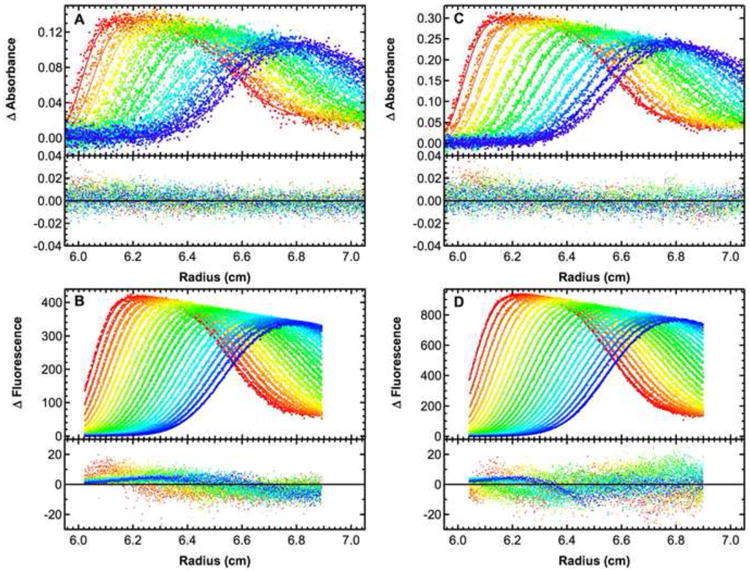
Absorbance (A and C) and fluorescence (B and D) data were recorded for samples loaded at concentrations of 164 nM and 327 nM. The data were subtracted in pairs to remove the time-independent noise and globally fit to a single ideal species model using SEDANAL to yield a best fit s =3.124 (3.121, 3.127) S. For clarity, only every third (absorbance) or fifth (fluorescence) scan is shown. The top panels show the data (points) and fit (solid lines) and the bottom panels show the residuals (points). The data were weighted by the estimated RMS noise level in the absorbance data and by the standard deviation at each point in the fluorescence data. Each data set was collected at a rotor speed of 50,000 RPM and a temperature of 20°C. The meniscus position for each sample was fixed based on the position of the negative spike observed in absorption intensity scans. The mass extinction coefficient of the labeled DNA for the absorbance data was obtained from the sequence. The mass extinction for the fluorescence data was fit and constrained to be equal for the two samples. Sedimentation coefficient confidence intervals were determined by incrementing the parameter until a critical variance is obtained based on the F-statistic using equation 34 in reference [22].

The other contribution to the nonrandom residuals is likely associated with drift in the laser excitation intensity. In conventional steady-state fluorimeters, it is customary to normalize the fluorescence intensity by a signal proportional to the excitation intensity to account for fluctuations in the lamp output. However, the AU-FDS detector does not provide such normalization and the laser intensity may change during the course of the sedimentation experiment. Slow drifts in signal intensity can result in systematic residuals in fits of sedimentation velocity data to Lamm equation solutions. The extent of this problem can be assessed by measuring the signal intensity of a nonsedimenting fluorophore as a function of time. For the instrument used to collect the data shown here, we detected a small (∼ 1%) linear decrease in the fluorescence signal over 5 hours, the typical time required for a sedimentation experiment. Another AU-FDS system exhibits a much larger slow upward drift in the signal amplitude of ∼10% with a half time of about 1.2 hours (data not shown). This signal change is associated with an increase in the laser intensity and can largely be eliminated by warming up the laser. Clearly, the AU-FDS system would benefit from a means to stabilize the laser light source and possibly normalize response of the detector using a standard sample.

In summary, the results presented here demonstrate that the AU-FDS fluorescence detector for the analytical ultracentrifuge is capable of providing precise and accurate sedimentation velocity data that are consistent with measurements performed using conventional absorption optics, provided the data are collected at appropriate concentrations and the optics are configured correctly. In contrast to a previous report that the fluorescence system systematically underestimates sedimentation coefficients by ∼ 10% [15], we find that the two detection systems yield consistent values.

References

- 1.Cole JL, Lary JW, Moody TP, Laue TM. Analytical ultracentrifugation: sedimentation velocity and sedimentation equilibrium. Methods in Cell Biology. 2008;84:143–179. doi: 10.1016/S0091-679X(07)84006-4. [DOI] [PMC free article] [PubMed] [Google Scholar]
- 2.Howlett GJ, Minton AP, Rivas G. Analytical ultracentrifugation for the study of protein association and assembly. Current Opinion in Chemical Biology. 2006;10:430–436. doi: 10.1016/j.cbpa.2006.08.017. [DOI] [PubMed] [Google Scholar]
- 3.Lebowitz J, Lewis MS, Schuck P. Modern analytical ultracentrifugation in protein science: a tutorial review. Protein Sci. 2002;11:2067–2079. doi: 10.1110/ps.0207702. [DOI] [PMC free article] [PubMed] [Google Scholar]
- 4.Laue TM, Stafford WF. Modern applications of analytical ultracentrifugation. Annu Rev Biophys Biomol Struct. 1999;28:75–100. doi: 10.1146/annurev.biophys.28.1.75. [DOI] [PubMed] [Google Scholar]
- 5.Cole JL, Hansen JC. Analytical Ultracentrifugation as a Contemporary Biomolecular Research Tool. J Biomolecular Techniques. 1999;10:163–176. [PMC free article] [PubMed] [Google Scholar]
- 6.Laue TM. Choosing Which Optical System of the Optima™ XL-I Analytical Ultracentrifuge to Use. Beckman-Coulter. 1996 [Google Scholar]
- 7.Schmidt B, Rappold W, Rosenbaum V, Fischer R, Riesner D. A fluorescence detection system for the analytical ultracentrifuge and its application to proteins, nucleic acids, and viruses. Colloid & Polymer Sci. 1990;268:45–54. [Google Scholar]
- 8.MacGregor IK, Anderson AL, Laue TM. Fluorescence detection for the XLI analytical ultracentrifuge. Biophys Chem. 2004;108:165–185. doi: 10.1016/j.bpc.2003.10.018. [DOI] [PubMed] [Google Scholar]
- 9.Crepeau RH, Conrad RH, Edelstein SJ. UV laser scanning and fluorescence monitoring of analytical ultracentrifugation with an on-line computer system. Biophys Chem. 1976;5:27–39. doi: 10.1016/0301-4622(76)80024-5. [DOI] [PubMed] [Google Scholar]
- 10.Kingsbury JS, Laue TM. Fluorescence-detected sedimentation in dilute and highly concentrated solutions. Meth Enzymol. 2011;492:283–304. doi: 10.1016/B978-0-12-381268-1.00021-5. [DOI] [PubMed] [Google Scholar]
- 11.Kroe RR, Laue TM. NUTS and BOLTS: applications of fluorescence-detected sedimentation. Anal Biochem. 2009;390:1–13. doi: 10.1016/j.ab.2008.11.033. [DOI] [PMC free article] [PubMed] [Google Scholar]
- 12.Lakowicz JR. Principles of Fluorescence Spectroscopy. Third. Springer; New York: 2006. [Google Scholar]
- 13.Stafford WF, Sherwood PJ. Analysis of heterologous interacting systems by sedimentation velocity: curve fitting algorithms for estimation of sedimentation coefficients, equilibrium and kinetic constants. Biophys Chem. 2004;108:231–243. doi: 10.1016/j.bpc.2003.10.028. [DOI] [PubMed] [Google Scholar]
- 14.Visser T, Groen F, Brakenhoff G. Absorption and scattering correction in fluorescence confocal microscopy. Journal of Microscopy. 1991;163:189–200. [Google Scholar]
- 15.Zhao H, Berger AJ, Brown PH, Kumar J, Balbo A, May CA, et al. Analysis of high-affinity assembly for AMPA receptor amino-terminal domains. J Gen Physiol. 2012;139:371–388. doi: 10.1085/jgp.201210770. [DOI] [PMC free article] [PubMed] [Google Scholar]
- 16.A Biomedical, Analytical Ultracentrifuge Fluorescence Detection System and Advanced Operating System User Manual. 2009 [Google Scholar]
- 17.Laue TM, Shah B, Ridgeway TM, Pelletier SL. Computer-aided interpretation of sedimentation data for proteins. In: Harding SE, Horton JC, Rowe AJ, editors. Analytical Ultracentrifugation in Biochemistry and Polymer Science. Royal Society of Chemistry; Cambridge, England: 1992. pp. 90–125. [Google Scholar]
- 18.Schuck P. Size-distribution analysis of macromolecules by sedimentation velocity ultracentrifugation and lamm equation modeling. Biophys J. 2000;78:1606–1619. doi: 10.1016/S0006-3495(00)76713-0. [DOI] [PMC free article] [PubMed] [Google Scholar]
- 19.Bailey MF, Angley LM, Perugini MA. Methods for sample labeling and meniscus determination in the fluorescence-detected analytical ultracentrifuge. Anal Biochem. 2009;390:218–220. doi: 10.1016/j.ab.2009.03.045. [DOI] [PubMed] [Google Scholar]
- 20.Lees EE, Gunzburg MJ, Nguyen TL, Howlett GJ, Rothacker J, Nice EC, et al. Experimental determination of quantum dot size distributions, ligand packing densities, and bioconjugation using analytical ultracentrifugation. Nano Lett. 2008;8:2883–2890. doi: 10.1021/nl801629f. [DOI] [PubMed] [Google Scholar]
- 21.Schuck P, MacPhee CE, Howlett GJ. Determination of sedimentation coefficients for small peptides. Biophys J. 1998;74:466–474. doi: 10.1016/S0006-3495(98)77804-X. [DOI] [PMC free article] [PubMed] [Google Scholar]
- 22.Johnson ML, Faunt LM. Parameter estimation by least-squares methods. Methods Enzymol. 1992;210:1–37. doi: 10.1016/0076-6879(92)10003-v. [DOI] [PubMed] [Google Scholar]
Associated Data
This section collects any data citations, data availability statements, or supplementary materials included in this article.