Understanding Heterogeneity in Price Elasticities in the Demand for Alcohol for Older Individuals

Abstract

This paper estimates the price elasticity of demand for alcohol using Health and Retirement Study data. To account for unobserved heterogeneity in price responsiveness, we use finite mixture models. We recover two latent groups, one is significantly responsive to price, but the other is unresponsive. The group with greater responsiveness is disadvantaged in multiple domains, including health, financial resources, education and perhaps even planning abilities. These results have policy implications. The unresponsive group drinks more heavily, suggesting that a higher tax would fail to curb the negative alcohol-related externalities. In contrast, the more disadvantaged group is more responsive to price, thus suffering greater deadweight loss, yet this group consumes fewer drinks per day and might be less likely to impose negative externalities.

1. INTRODUCTION

Federal excise taxes on alcohol have not risen since 1991, and the real tax rate has been declining. However, many states are now actively considering raising taxes on alcohol to meet revenue shortfalls.¹ The rising attention to increasing alcohol taxes may be caused by the success of state and federal taxes on tobacco in boosting revenue. However, the analogy is not perfect. Although any smoking is harmful, most drinkers consume alcohol without harming their own health and without imposing externalities; only a sub-group misuse alcohol. Thus, the potential heterogeneity in impact of taxes across types of drinkers (those imposing internalities and/or externalities) is important to determine empirically.

The price elasticity of demand for alcohol is a significant determinant of the potential welfare effects of increasing alcohol taxes regardless of motive for increasing the tax on alcohol.² The ability for taxes to raise revenue, reduce externalities, improve the health of the public, or act as a pre-commitment device³ all depend on the price elasticity of demand for alcohol. However, it is not just the average price elasticity that matters. To reduce the alcohol-related externalities associated with those who misuse alcohol, while preserving the utility derived by the majority of drinkers who do not impose externalities, those most likely to impose externalities should be most responsive to taxes, whereas those who are enjoying alcohol without external costs should be least responsive.⁴

Although much of the economics literature on alcohol is aimed at youth drinking, we focus on older individuals and the potential impact of price on this population. Older drinkers are an important set of drinkers in part because of critical interactions between alcohol and both disease and associated medications— both of which are more common in older populations (Williams, 1984; Abrams and Alexopoulos, 1977). Although older individuals drink less than younger ones, they attain higher blood alcohol content for a given amount of alcohol consumed, and for any given level of blood alcohol, they have an intensified sensitivity to ethanol (Vestal et al., 1977; Vogel-Sprott and Barrett, 1984). Furthermore, balance, gait, cognition, and driving ability can be disturbed by alcohol consumption, and these issues are of greater concern as one ages (Williams, 1984).

In this paper, we estimate the price elasticity of demand for alcohol explicitly allowing for differences in elasticities across complex sub-groups of individuals. We use a finite mixture model (FMM) to allow the price elasticity to vary by latent sub-groups that could not be identified by using simple groups such as by age, gender, or consumption level. We find that there are important differences in price elasticity that are masked in a single equation method but revealed in a two-component FMM. FMM allows prior and posterior characterization of the latent groups. By characterizing these two groups of individuals, we find that some of the difference between the groups can be explained by variation in demographics as well as health, financial, and behavioral factors. We show that this group-level variation is not only caused by addiction to alcohol. These findings are relevant to alcohol tax policy as it applies to older individuals.

We add to the literature in multiple dimensions. First, the topic of alcohol taxes is of current policy concern, given the latest wave of proposed state level tax hikes on alcohol. Second, we examine older individuals, a group that has received relatively little empirical analysis with respect to alcohol consumption. Third, our use of FMM allows heterogeneity across latent groups, identifying differences which would otherwise be masked by pooling. The heterogeneity that we find across latent groups is relevant to policy goals. Finally, we examine the role of cognition and physical health, financial factors, and behavioral factors in explaining differences across the latent groups.

1.1. Background on price elasticity

There is considerable range in estimates of the price elasticity of demand for alcohol, with variation likely attributable to data type (aggregated or individual) and source (national, cross-sectional), age groups (often youths), measure of consumption (sales or quantity and frequency), price (beer, wine, or spirits, separately or an average), use of tax rate versus price, econometric methods, and other factors. A full literature review is beyond the scope of this study, given the long history of studies, but we will start by discussing a meta-analysis to set the stage and then discuss those studies that are most relevant to the current study. Wagenaar et al. (2009) conduct a formal meta-analysis and review of 1003 separate estimates of the price and tax elasticities of demand for alcohol from 112 studies.⁵ They conclude that alcohol prices and tax rates significantly reduce consumption of alcohol and that the average price elasticity from studies using aggregate data is −0.44 and much lower (but not reported) from studies using individual level data. Using the simple mean effect across all of the studies, they find price elasticities for beer, wine, and spirits to be −0.46, −0.69, and −0.80, respectively.⁶ Using more sophisticated meta-analysis techniques, including weighting the study outcomes by the precision of the estimates, they find the elasticities for beer, wine, and spirits to be −0.17, −0.30, and −0.29, respectively. For heavy drinkers, the elasticity is estimated to be −0.28 across all drink types.

Although this meta-estimate is extremely useful, an estimate of the average impact masks potential heterogeneity in response to alcohol taxes. Several studies have found evidence of heterogeneity. Using data from the Health Promotion and Disease Prevention supplement to the 1993 NHIS, Kenkel (1996) finds price elasticities of −0.828 for male subjects and −0.710 for female subjects when the number of days drinking under four drinks per day is used as the outcome. The biggest difference by gender is found using the outcome of days using five or more drinks per day (heavy drinking); Kenkel finds an elasticity of −0.5 for men and more than double this for women (−1.3).⁷

Two extant studies are more closely related to our current study. Using the National Health Interview Survey, Manning et al. (1995) examine whether the price elasticity of demand for alcohol varies by consumption levels. Their measures of alcohol consumption include the following: a binary indicator of being a current drinker, the average number of ounces of ethanol consumed per day (derived from data on quantity and frequency of drinks), and a measure of five of more drinks per day. They use a two-part model to separate the decision to drink from the quantity consumed conditional on being a drinker, finding an overall price elasticity of−0.80.⁸ However, the price elasticity for drinks, conditional on being a drinker, is not significantly different from zero, whereas price significantly affects the decision to drink (elasticity of −0.55). Quantile regression is used to address the question of heterogeneity of elasticity across drinkers based on their level of consumption, finding that the most price responsive drinkers are the moderate drinkers. The median drinker has a price elasticity of −1.19. The lowest quantile drinker has a price elasticity of −0.55, whereas the two highest quantile drinkers have elasticities of −0.49 and 0.12, respectively; all but the latter are significant. Manning et al. conclude that there is heterogeneity in the price elasticities and that failure to differentiate these groups could conceal important policy relevant information.

Dave and Saffer (2008) use both the Panel Study of Income Dynamics (PSID) and the Health and Retirement Study (HRS) to examine whether the beer tax elasticity of demand for alcohol varies by risk preference. They find that a higher risk aversion reduces alcohol consumption but that the tax elasticity of demand does not vary by a binary risk preference class. Furthermore, they find that older individuals are more tax responsive (using beer tax measures) than younger individuals (comparing age groups within the PSID). Participation elasticity is estimated to be between −0.05 and −0.04 for younger individuals in the PSID and between −0.22 and −0.11 for HRS participants over age 55. Tax elasticities conditional on being a drinker, using the average number of drinks per day as the dependent variable, are estimated to be between −0.10 and −0.08 depending on the specification. Chronic drinkers have a tax elasticity on this intensive margin of −0.27, indicating that even heavy drinkers are at least as, if not more, price sensitive than other drinkers. This contrasts to the findings of Manning et al. in which moderate drinkers were found to be the most price sensitive. Both the Manning et al. (1995) and Dave and Saffer (2008) studies suggest that there may be some heterogeneity in the demand for alcohol. We address this directly using the FMM approach to allow heterogeneity in response across latent groups.

1.2. Data

We use data from the HRS, a nationally representative longitudinal survey of individuals over 50 years and their spouses. At baseline in 1992, HRS participants included 12 652 individuals from 7702 households. The HRS initially sampled persons in birth cohorts 1931 through 1941 in 1992 and then conducted follow-up interviews biennially. In 1998, persons from the 1924–1930 cohort and the 1942–1947 cohort were added to the original sample. In 2004, persons from the 1948–1953 cohort were added to the survey.⁹ The HRS sample was selected under a multi-stage area probability sample design and oversampled Black and Hispanic respondents as well as residents of Florida.¹⁰ All regressions are weighted using person level analysis weights from the RAND HRS data that account for sampling design and adjust for sample attrition and mortality. They correspond to the US population as measured by the March CPS for the survey year.¹¹

Our initial sample includes all individuals who were surveyed in 1996 through 2004 and consists of 97250 person-year observations. We exclude individuals under 51 years of age. In addition, we exclude observations for which data were missing on any of the following variables: drinks per day, state and census region of residence, alcohol price for the corresponding state-year, age, race, gender, height, and years of education. Our final sample consists of 65 002 person-wave observations.

1.2.1. Dependent variable

The HRS asked respondents whether they ever drink any alcoholic beverages such as wine, beer, or liquor. Approximately 46% of the sample answered yes to this question. If they answered yes, then they were asked how many drinks they have per day on the days that they drink. This measure does not capture all aspects of alcohol consumption (e.g. days drinking); however, it may be a good proxy for the most problematic drinking as it is the number of drinks per occasion that engenders risky behavior.¹² This question was not asked in the first two waves of the HRS, so we used data only from the third through seventh wave of the survey. The average number of drinks for the full sample of 65 002 observations is 0.68 and for drinkers only, it is 2.08.

1.2.2. Independent variables

The main specification controls for age, race, gender, height in meters, log of household income (1992$), and years of education. To allow for nonlinear effects of age, we created age categories with a reference category of ages 51–61. We also included binary indicators for the individual’s census region of residence and year. The reference group for census region was Pacific, and that for year was 1996. In other regressions, we also account for labor force status (retired, not working, with working the omitted category) and marital status. Summary statistics for the analysis sample are shown in Table I. We also present summary statistics for the variables included in the main specification for the initial HRS sample and test for significant differences from the analysis sample.

Table I.

Summary statistics

	Analysis sample		Health and retirement study sample		Test for difference in means
	Mean	Standard deviation	Mean	Standard deviation	p-value
Age 0–50	0.000		0.010		0.000
Age 51–60	0.401		0.366		0.000
Age 61–70	0.296		0.276		0.000
Age 71–80	0.208		0.234		0.000
Age 81+	0.096		0.114		0.000
Black	0.097		0.093		0.216
Other race	0.031		0.038		0.003
Male	0.453		0.449		0.015
Height	1.695	0.001	1.692	0.001	0.000
Years of education	12.395	0.084	12.363	0.076	0.504
Drinks per day	0.680	0.013
Average price per ounce of ethanol	8.304	0.049
Married or partnered	0.662
Household income (in 10000 1992 USD)	4.643	0.121
Binge drinking	1.506	0.066
Risk aversion (imputed)	3.273	0.015
Financial planning horizon (imputed)	3.022	0.019
Retired	0.414
Not working	0.146
Number of health conditions	1.743	0.015
Difficulty paying bills	2.097	0.027
Ongoing financial strain	1.647	0.024
Cognition	14.534	0.051
Observations	65,002		97,250

The number of observations is not the same for all variables in the analysis sample as well as the HRS sample.

Estimated statistics account for p-weights, stratification, and clustering at the Primary Sampling Unit (PSU) level and were calculated using the svy:mean command in STATA.

1.2.3. Alcohol price

We merged the HRS data with state-level alcohol prices standardized per ounce of ethanol using standard drink size for each wine, beer, and spirits and the concomitant ounces of ethanol per drink. Adjustments were made for state variation in cost of living, and prices were adjusted for inflation over time.¹³ In our primary results, we used the log of the three price equally weighted to develop an average price rate measure.¹⁴

1.2.4. Health measures

We use two measures of health: the number of chronic health conditions as a proxy for physical health, and a cognitive ability score—the higher the score, the greater the cognitive ability. See the data appendix for more detail on these measures.

1.2.5. Financial measures

In 2004, HRS included a self-administered questionnaire for a random sample of non-institutionalized respondents upon completion of a core in-person interview. The questionnaire asked how difficult it is for the respondent/respondent’s family to meet monthly payments on his/their bills. Answers were coded on a five-point scale, with 1 representing ‘not at all difficult’ and 5 representing ‘completely difficult’. Respondents also were asked about ongoing financial strain that had lasted 12 months or longer and indicated how upsetting it has been on a four-point scale, with 1 representing ‘no, didn’t happen’ and 4 representing ‘yes, very upsetting’.

1.2.6. Behavioral factors

We use measures of risk-aversion and financial planning horizon; however, these variables are available for only a subset of the sample. To measure risk preferences, the HRS asked respondents to choose among four different gambles. Based on respondent choices, we created a risk aversion index ranging from 1 to 4, with 4 being the most risk averse. More detail on these variables is provided in the Appendix.

1.2.7. Binge drinking

The HRS asked respondents the number of days that they had four or more drinks on one occasion, in the last 3 months.

1.3. Econometric methods

The basic econometric model for number of drinks per day (DRINKS), an integer valued variable, is given by the following:

$$E\left({\text{DRINKS}}_i|\text{ln}{\text{PRICE}}_i,X_i\right)=\exp \left(\alpha \text{ln}{\text{PRICE}}_i+X{’}_i\beta \right)$$ (1)

where lnPRICE_i is the logarithm of the average alcohol price corresponding to observation i, and X denotes socioeconomic characteristics. Equation (1) is first estimated by Poisson and negative binomial (NB) regressions. In these models, the coefficient α is the price elasticity of alcohol consumption. However, if DRINKS is drawn from distinct subpopulations, the estimate of α is the average of the effects across subpopulations and may hide substantive differences in α across the subpopulations. Thus, we also estimate Equation (1) using a number of FMMs with Poisson-distributed subpopulations. The main identification assumption for these models is that price is exogenous to the individual.

In the FMM, the random variable DRINKS is postulated as a draw from a population, which is an additive mixture of C distinct classes or subpopulations in proportions π_j such that

$$g\left({\text{DRINKS}}_i|\theta ,\pi \right)={\displaystyle \sum _{j=1}^C{\pi }_j{f}_j\left({\text{DRINKS}}_i|{\theta }_j\right),0\le {\pi }_j\le 1},{\displaystyle \sum _{j=1}^C{\pi }_j=1}$$ (2)

Equation (2) assumes that the proportions π_j are constant across observations. The mixture density in the Poisson mixture for DRINKS is given by the following:

$$f_i\left({\text{DRINKS}}_i|{\theta }_j\right)=\frac{{\lambda }_{ji}^{{\text{DRINKS}}_i}\exp \left(-{\lambda }_{ji}\right)}{{\text{DRINKS}}_i!},j=1,2,\dots ,C.$$ (3)

where ${\lambda }_{ji}=\text{exp}{({\alpha }_{j}ln{\text{PRICE}}_i+X’}_i{\beta }_j)$. We estimate models in which C=2 and C=3. There is no evidence in our sample of four distinct components.

The FMM provides a representation of heterogeneity in a small, finite number of latent classes, each of which may be regarded as a ‘type’ or a ‘group’. Two studies (Heckman and Singer, 1984; Laird, 1978) suggest that estimates of such models may provide good numerical approximations even if the underlying mixing distribution is continuous. In addition, the finite mixture approach is semi-parametric— it does not require any distributional assumptions for the mixing variable—and, under suitable regularity conditions, is the semi-parametric maximum likelihood estimator of the unknown density (Lindsay, 1995).¹⁵ A finite mixture characterization is especially attractive if the mixture components have a natural interpretation. However, a finite mixture may be simply a way of flexibly and parsimoniously modeling the data, with each mixture component providing a local approximation to some part of the true distribution.¹⁶

We also estimate a two-component model in which the (prior) component probabilities are of the form:

$${\pi }_{ij}=\text{logit}(Z_i|\delta ),0\le {\pi }_{ij}\le 1, {\displaystyle {\sum }_{j=1}^C{\pi }_{ij}}=1$$ (4)

The prior component probability now depends on observables Z and so varies across observations.

The FMMs are estimated using maximum weighted likelihood, that is, the contribution of each observation to the log likelihood is weighted by its sampling weight. In addition, we obtain robust standard errors that are clustered at the state level.¹⁷

We use our finite mixture parameter estimates to calculate the posterior probability of being in each of the latent classes. We use Bayes’ Theorem to calculate the posterior probability of membership in each class, conditional on all observed covariates and outcome, as

$$\mathrm{Pr}({\text{DRINKS}}_i\in k|\theta ,{\text{DRINKS}}_i)=\frac{{\pi }_k{f}_k({\text{DRINKS}}_i|\theta )}{{\displaystyle \sum _{j=1}^C{\pi }_j{f}_j({\text{DRINKS}}_i|\theta }}),\forall k=1,2,\dots ,C$$ (5)

We use the estimated posterior probabilities to explore the determinants of class membership.

Several potentially attractive alternative econometric strategies are worth discussing; the use of quantile regression methods, dealing with the large fraction of zeros using two part models, and direct interactions of key variables with price. Quantile regressions have been used in similar contexts to study heterogeneous responses to treatments, but they have two limitations vis-à-vis FMMs in our context. First, quantile regressions are not well behaved in the context of count data.¹⁸ Second, although quantile regression methods may detect heterogeneous responses, they provide no way to characterize the source of the heterogeneity.

Two-part models are ubiquitous in the health economics literature to deal with potential heterogeneity between users and non-users when the distribution of the outcome includes a substantial fraction of zeros. Although our data do include a substantial fraction of zeros, the two-part model is less attractive than the finite mixture for two reasons. First, the two-part model may be thought of as a special case of the FMM in which one of the components has a degenerate distribution at zero. Second, because occasional drinkers go back and forth between no drinks and light drinking, the distinction between use and non-use may be less attractive than the distinction between low and high use, which is the distinction that the FMM makes.

Another approach that allows for differential price effects across subpopulation would estimate models in which price is interacted directly with key independent variables, for example, gender. Although this approach too could be of interest, the FMM approach is more general and allows analysis by complex latent groups, not just, for example, gender differences.

2. RESULTS

2.1. Model selection

To determine the model that best fits the data, we estimated Poisson and NB models along with a number of FMMs and compared likelihood-based model selection criteria including Akaike Information Criterion and Bayesian information criterion (BIC) and a measure of the closeness of fit of the estimated density to the empirical density, which we label root mean square error of probabilities (RMSEP). These results are reported in Table IIa and b.

Table II.

Selection criteria for various models

	Log-likelihood	Degrees of freedom	Akaike information criterion	Bayesian information criterion	Root mean square error of probabilities
2a. Single equation models
Poisson	−2.83e+ 08	22	5.66e+08	5.66e+08	0.0520
Negative binomial	−2.45e+ 08	23	4.91e+08	4.91e+08	0.0136
2b. FMMsa
2-component, constant probability	−2.43e+ 08	41	4.87e+08	4.87e+08	0.0106
3-component, constant probability	−2.40e+ 08	41	4.79e+08	4.79e+08	0.0105
2-component, variable probability	−2.41e+ 08	41	4.82e+08	4.82e+08	0.0073

^aFinite mixture models with negative binomial components failed to converge in most specifications. In some specifications that did converge, one or more of the estimated overdispersion parameters were close to zero, implying that the component density was really a Poisson. Therefore, in what follows, the finite mixture models all have Poisson components.

FMM, finite mixture model.

Among the single class models, we find that the NB model fits the data substantially better than the Poisson model (Table IIa). However, FMMs with NB components failed to converge in most specifications. In some specifications that did converge, one or more of the estimated overdispersion parameters were close to zero, implying that the component density was really a Poisson. Therefore, in what follows, the FMMs all have Poisson components.

Next, we calculated information criteria for the Poisson–FMM and find that it is a superior specification to the single component NB model. The results also show that there is relatively little difference between the two-component FMM with constant probabilities, the three-component FMM with constant probabilities, and the two-component smoothly mixing FMM (with probabilities specified as a function of covariates). In fact, the likelihood-based criteria produce different decisions as compared with the RMSEP (Table IIb). The BIC suggests that the three-component FMM is best, but the RMSEP suggests that the two-component model with variable probabilities fits the distribution better. As we shall see below, in the three-component model, two of the price elasticities are not significantly different from each other; thus, we focus on the two-component smoothly mixing FMM as our preferred specification. The difference in model fit between a standard NB regression model and the FMM also can be seen in Figure 1, which presents the observed distribution of the dependent variable along with predicted probabilities from the two models.

Figure 1.

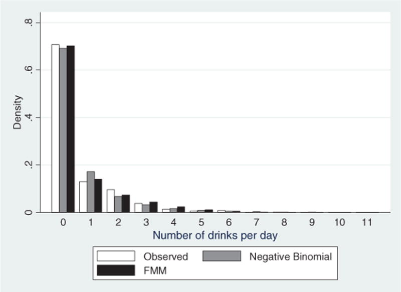
Observed and predicted probabilities from negative binomial and finite mixture models

2.2. Price effects

Estimating a single component NB regression, we find that price has a significant (p < 0.01) impact on the number of drinks consumed with a coefficient of −0.402 (Table III, column 1). This estimate falls within the range of estimates reported by Wagenaar et al.

Table III.

Heterogeneity in price elasticity of alcohol demand

	Negative binomial	FMM component 1	FMM component 2	FMM prior probability of component 1	Test of difference between components—p-value
Log alcohol price	−0.402*** (0.152)	−1.686*** (0.651)	0.0131 (0.0863)		0.0123
Age 61–70	−0.249*** (0.0299)	0.0551 (0.0981)	−0.164*** (0.0392)	0.178*** (0.0573)	0.0229
Age 71–80	−0.586*** (0.0462)	0.149 (0.130)	−0.467*** (0.0495)	0.356*** (0.102)	0.000
Age 81+	−1.039*** (0.0432)	−0.289 (0.179)	−0.939*** (0.0737)	0.310** (0.135)	0.0002
Height	0.168 (0.308)	0.720 (0.510)	0.233 (0.242)	−0.0146 (0.483)	0.3081
Years of education	0.0432*** (0.00644)	0.250*** (0.0315)	−0.0672*** (0.00630)	−0.124*** (0.0156)	0.000
Black	−0.351*** (0.0564)	−2.367*** (0.638)	−0.121* (0.0688)	0.183 (0.125)	0.0002
Other race	−0.227*** (0.0847)	−4.782 (11.06)	−0.0100 (0.135)	0.166 (0.220)	0.6631
Male	0.902*** (0.0627)	−0.00306 (0.127)	0.448*** (0.0361)	−0.850*** (0.0828)	0.0010
Constant	−0.618 (0.608)	−2.407 (2.036)	0.802** (0.404)	2.739*** (0.720)
Observations	65,002	65,002	65,002	65,002
Mean predicted y		0.13	1.86
Mean posterior probability		0.728	0.272

Regressions also include census region of residence and year dummies.

Standard errors in parentheses; regressions are weighted, and robust standard errors are clustered at the state level.

^*p<0.1

^**p<0.05

^***p<0.01.

When we estimate the smoothly mixing two-component FMM, we find that for the first and largest group (72.8% of the sample), price also has a significant impact on the number of drinks consumed (p < 0.001) with a coefficient of −1.686 (Table III, column 2). In contrast, for the second, smaller group (27.2% of the sample), price is not significant, and the coefficient is 0.0131 (Table III, column 3). The price elasticities are significantly different between these two groups (p < 0.012), and this suggests that the single component model is composed of two unlike groups. The larger group (Component 1) consumes 0.13 drinks per day on average, whereas the smaller group (Component 2) has an average consumption of 1.86 drinks per day.¹⁹ This heterogeneity is masked in the single equation estimation approach. Figure 2, which graphs the number of drinks for each component, demonstrates graphically that the determination of the two components is not based on drinking status alone; many members of the less responsive group (Component 2), for instance, consume 0 or 1 drink per day.

Figure 2.

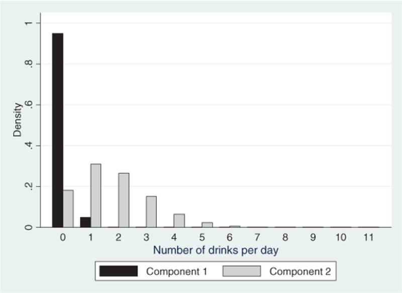
Predicted component probabilities from finite mixture model

For purposes of comparison, we present the price elasticities from the Poisson, NB, and each of the three FMMs in Table IV. The FMM with three components (with constant probabilities) identified one component with a significant price elasticity of −1.124 and two components with insignificant price elasticities (Table VI). The price elasticities in the second and third component were not significantly different from each other, suggesting that the two-component FMM captures the important heterogeneity in the price responsiveness. Overall, the price elasticities from each of the FMM are qualitatively quite similar to each other.

Table IV.

Comparison of price elasticity estimates across models

	Overall	FMM component 1	FMM component 2	FMM component 3	N	Test for difference between componentsp-value
Poisson	−0.297** (0.129)				65,002
Negative binomial	−0.402*** (0.152)				65,002
2-component, variable probability		−1.686*** (0.652) [0.728]	0.013 (0.086) [0.272]		65,002	0.0123
2-component, constant probability		−0.951*** (0.281) [0.735]	−0.070 (0.092) [0.265]		65,002	0.0030
3-component, constant probability		−1.124*** (0.327) [0.651]	−0.097 (0.072) [0.327]	0.090 (0.226) [0.022]	65,002	0.0011a 0.0033b 0.4329c

Standard errors in parentheses, sample proportion belonging to component in square brackets.

^aTest between components 1 and 2.

^bTest between components 1 and 3.

^cTest between components 2 and 3.

^*p<0.1

^**p<0.05

^***p<0.01.

Table VI.

Robustness check—models that include state laws

	FMM component 1	FMM component 2	FMM prior probability of component 1	Test for difference between the components—p-value
Log alcohol price	−1.652** (0.662)	−0.00969 (0.0883)		0.0162
Blood alcohol content	0.147 (0.201)	−0.00237 (0.0302)		0.4715
License revocation	−0.0548 (0.325)	−0.0886*** (0.0321)		0.9150
Zero tolerance	−0.187 (0.170)	−0.0598 (0.0487)		0.4583
Age 61–70	0.0492 (0.0990)	−0.164*** (0.0392)	0.178*** (0.0567)	0.0290
Age 71–80	0.145 (0.130)	−0.466*** (0.0487)	0.363*** (0.100)	0.000
Age 81+	−0.294* (0.175)	−0.941*** (0.0756)	0.312** (0.136)	0.0002
Height	0.735 (0.507)	0.223 (0.241)	−0.0153 (0.477)	0.2795
Years of education	0.249*** (0.0307)	−0.0673*** (0.00632)	−0.123*** (0.0154)	0.000
Black	−2.374*** (0.626)	−0.124* (0.0700)	0.178 (0.127)	0.0002
Other race	−4.483 (8.208)	−0.00949 (0.135)	0.165 (0.220)	0.5810
Male	−0.0164 (0.127)	0.445*** (0.0370)	−0.861*** (0.0847)	0.0007
Constant	−2.381 (2.020)	0.974** (0.428)	2.748*** (0.709)
Observations	65,002	65,002	65,002
Mean predicted y	0.13	1.86
Mean posterior probability	0.729	0.271

Regressions also include census region of residence and year dummies.

Standard errors in parentheses; regressions are weighted, and robust standard errors are clustered at the state level.

^*p<0.1

^**p<0.05

^***p<0.01.

2.3. Prior probability

In the prior probability equation of Table III (column 2), we use a basic set of exogenously determined, socio-economic variables to classify observations into the latent subgroups. The results indicate that individuals who are older, less educated, and female are more likely to belong to the latent Component 1, the more responsive group.²⁰

2.4. Posterior probability

Using the empirically established groups from the FMM regression results, we use a richer set of variables to characterize the two latent components. Our descriptive analysis of posterior probabilities aims to identify factors that are correlated with group membership (see Table V). In these analyses, we include variables that extend beyond the standard socio-economic and demographic measures to include behavioral measures and other variables that may not be exogenous (e.g. marital status and income).²¹

Table V.

Posterior probability of component 1

	(1)	(2)	(3)	(4)	(5)	(6)
Married or partnered	0.0121* (0.00662)		0.0393* (0.0210)		0.0407 (0.0284)
Log household income	−0.0115*** (0.00172)		−0.0113** (0.00439)		−0.0108** (0.00476)
Cognition	−0.00230*** (0.000493)		−0.00125 (0.00192)		−0.00125 (0.00268)
Number of health conditions	0.0221*** (0.00189)		0.0153*** (0.00523)		0.0190** (0.00745)
Retired	0.00128 (0.00775)		−0.00202 (0.0140)		0.00439 (0.0208)
Not working	0.0162** (0.00773)		0.0389** (0.0143)		0.0695*** (0.0181)
Difficulty paying bills			0.00761 (0.00666)		0.0255* (0.0137)
Ongoing financial strain			0.0113 (0.00896)		−2.28e-05 (0.0150)
Risk					−0.0159 (0.0112)
Financial planning horizon					0.00304 (0.00859)
Age 61–70	0.0229*** (0.00551)	0.0349*** (0.00468)	0.0396** (0.0152)	0.0383*** (0.0124)	0.0405* (0.0220)	0.0420** (0.0181)
Age 71–80	0.0400*** (0.00677)	0.0639*** (0.00579)	0.0599** (0.0254)	0.0626*** (0.0189)	0.0591 (0.0395)	0.0586* (0.0312)
Age 81+	0.0181** (0.00888)	0.0503*** (0.00711)	0.0600* (0.0333)	0.0548** (0.0256)	0.0353 (0.0880)	0.0259 (0.0827)
Height	−0.00310 (0.0535)	−0.00884 (0.0536)	−0.0241 (0.0879)	−0.0246 (0.0942)	−0.0147 (0.117)	−0.0104 (0.118)
Years of education	−0.0188*** (0.00159)	−0.0229*** (0.00159)	−0.0174*** (0.00268)	−0.0229*** (0.00295)	−0.0154*** (0.00515)	−0.0228*** (0.00468)
Black	0.0195 (0.0121)	0.0315** (0.0127)	−0.00270 (0.0236)	0.00175 (0.0201)	−0.0171 (0.0361)	−0.0116 (0.0314)
Other race	0.0276* (0.0144)	0.0357** (0.0153)	−0.0670 (0.0539)	−0.0533 (0.0588)	−0.131** (0.0568)	−0.109 (0.0679)
Male	−0.172*** (0.00845)	−0.173*** (0.00753)	−0.143*** (0.0184)	−0.147*** (0.0201)	−0.144*** (0.0235)	−0.150*** (0.0229)
Constant	1.097*** (0.0890)	1.039*** (0.0863)	1.033*** (0.143)	1.060*** (0.146)	0.972*** (0.216)	1.009*** (0.202)
N	54,489	54,489	7,449	7,449	3,881	3,881
R2	0.128	0.117	0.107	0.095	0.109	0.089

Regressions also include census region of residence and year dummies.

Standard errors in parentheses; regressions are weighted, and robust standard errors are clustered at the state level.

^*p<0.1

^**p<0.05

^***p<0.01.

2.4.1. Health

Individuals with more adverse health conditions are significantly more likely to be in the responsive group. Those with lower cognitive ability also are more likely to be in the price responsive group, but this is significant only in the first specification. Thus, those more responsive to price are more likely to be in poorer health.

2.4.2. Financial issues

The results relating to income, not working, and difficulty paying bills indicate that those who are responsive are likely to be financially disadvantaged compared with the non-responsive component. Difficulty paying bills is positively and significantly associated with the probability of being in the responsive group, whereas higher income is negatively associated with being in the responsive group. Ongoing financial strain and retired are insignificant.

2.4.3. Risk aversion

Risk aversion is insignificant in predicting membership of the components; however, note the smaller sample size because of the fewer number of persons who were asked about risk aversion. As a point of comparison, Dave and Saffer (2008) found that risk aversion was negatively associated with alcohol consumption, but they also found that the price elasticity did not differ across low-risk and high-risk groups.

2.5. Robustness checks

2.5.1. Binge drinking

To examine whether differences across the components were solely in drinking behavior, we regressed the posterior probability of being in group 1 on binge drinking, controlling for the variables listed in Table V. The coefficient on binge drinking is −0.0125 (significant at 1%). However, including binge drinking in the regression has little qualitative impact on the significance and sign of the other independent variables. This suggests that, although binge drinking is significantly correlated with membership in component 2, it does not explain all the variation across the two components.

2.5.2. State sentiment

In Table VI, we include three state level drunk driving laws to test for the impact of state sentiment on the estimate of price elasticity.²² The state-varying laws are as follows: blood alcohol content (BAC) limit of 0.08 or under, license revocation, and zero tolerance (see Appendix A for details). Including these laws helps to address the possibility that state tax rates and levels of alcohol consumption are simultaneously determined, at least in part, by differences in state sentiment toward alcohol consumption, which could bias the results. Because zero tolerance laws affect only those under age 18, this law may offer the purest control for sentiment uncontaminated by a direct effect on older individuals. Estimates of the price elasticity are affected very little by inclusion of these variables.

2.5.3. Separate price on each beer, wine, and spirits

We also compare results using the price on each beer, wine, and spirits in separate regressions. The price elasticities obtained in these regressions are reported in Table VII. They show that price elasticities are qualitatively similar across these specifications and also those using average prices. Because we do not have the delineation of consumption by type of alcohol, we consider these estimates as specification checks not the preferred specifications.

Table VII.

Comparison of price elasticity estimates across models

	FMM component 1	FMM component 2	N	Test for difference between components p-value
Beer	−1.344** (0.548) [.729]	−0.0149 (0.0773) [0.271]	65,002	0.0206
Wine	−1.504*** (0.563) [0.731]	0.141 (0. 119) [0.269]	65,002	0.0059
Liquor	−0.932*** (0.268) [0.770]	−0.0480 (0.0886) [0.230]	65,002	0.0022

Standard errors in parentheses, sample proportion belonging to component in square brackets.

^aTest between components 1 and 2.

^bTest between components 1 and 3.

^cTest between components 2 and 3.

^*p<0.1

^**p<0.05

^***p<0.01.

2.5.4. Maximum number of drinks

Our results also are robust to an alternative specification, in which we limited the maximum number of drinks to be 15. We also estimated models that included alcohol price adjusted for sales tax. Our results are robust to the inclusion of this variable; the price elasticity for component 1 was −1.504 (significant at 5%), and that for component 2 was 0.0418 (insignificant).²³

2.5.5. Non-drinkers

In an alternative specification, we excluded consistent non-drinkers, that is, individuals who reported no drinking in any waves of data.²⁴ The price elasticity for component 1 was −0.625 (significant at 1%), and that for component 2 was 0.102 (insignificant). This limited sample analysis did not fit as well as our preferred specification, which retains the non-drinkers in the sample. The latter considers non-drinkers to be at risk of becoming drinkers and allows the estimation approach to determine the composition of the latent classes rather than simply eliminating part of the sample.

3. CONCLUSION

We find that there is important heterogeneity in the impact of alcohol price on consumption and suggest that this heterogeneity has welfare implications for an older sample of individuals. For the majority of these older individuals, price is a significant determinant of demand for alcohol, and demand is quite elastic (elasticity of −1.686; p < 0.01). Most estimates of alcohol price elasticity, in contrast, suggest that the demand is inelastic; we find this too in our single equation regression (elasticity of 0.402; p < 0.01). For the other smaller group, prices do not significantly affect consumption. Those who are most responsive to price seem to be a more disadvantaged group in terms of education, health, cognition, and financial resources. The more responsive group is more likely to be non-white, female, married, and older and to consume less alcohol.

There is growing political support for increased alcohol taxes; however, we are cautious about predicting welfare gains to alcohol tax hikes with regard to older individuals.²⁵ Revenue may be raised at the cost of welfare loss for many older individuals but with little reduction in externalities. Heavier drinkers are more likely to impose negative externalities than the lighter drinkers. However, our results indicate that the heavier drinking group is insensitive to price; thus, higher taxes would be unlikely to reduce negative externalities for older drinkers.²⁶ In contrast, for the largest group of individuals, composed of moderate-to-low drinkers, the higher tax will reduce their alcohol consumption, resulting in a utility loss and loss of potential health benefits of alcohol (Thun et al., 1997²⁷), yet it is unlikely to reduce externalities.

Pogue and Sgontz (1989) also suggest that heterogeneity is critical in welfare analyses of alcohol taxes. They posit two groups of drinkers, non-abusers and addicted, suggesting the addicted may welcome a reduction in their consumption as they suffer from a compulsion that makes them unable to stop drinking even when they want to. Evidence on differential price elasticity of demand across groups was required for their welfare analysis, but such estimates were not available to them at that time. We provide evidence on this point for older individuals.

We add to the literature on alcohol taxes, which is of current policy concern, by examining the effect on older individuals. This is a group that has received relatively little empirical analysis with respect to alcohol consumption, but there are important differences in consumption patterns, interactions, and impact of alcohol. Importantly, we identify significant differences in price elasticities across latent groups that otherwise would be masked by pooling these disparate groups. We also examine whether cognitive ability, physical health, financial factors, and behavioral factors are critical in defining these groups. Both the heterogeneity and the differences in characteristics across the groups are policy relevant. Our measure of alcohol consumption, number of drinks per day, is better than some other measures in that we avoid the concern about double counting drinking events that can occur in the typical quantity and frequency questions. However, we recognize that data on quantity and frequency would have advantages as well.

Despite these strengths, there are several limitations of the study to acknowledge. First, we do not have direct measures on alcohol-related externalities such as drunk driving. Our measure of alcohol is somewhat limited. In addition, we do not have data separately by wine, beer, and spirits. Also, we weight the prices of beer, wine, and spirits equally. Using state sales levels to weight prices, as others have performed, would be inappropriate because the older population has a different distribution of drink types. Another potential weakness is in terms of policy implementation; the groups with different elasticities are not directly observable (although we can describe their characteristics). However, the overall caution that the welfare impact of higher taxes for this group might not be beneficial does not depend on identifying specific individuals. To implement specific policies, additional research would be warranted.

This paper unmasks important heterogeneity in the price elasticity of demand for alcohol across groups. The results suggest caution, at least for this older population, with respect to predicting policy gains from higher alcohol taxes. Although the specific results apply to an older population, the general message is that attention to heterogeneity in the responsiveness to tax is critical in analysis of welfare effects of alcohol taxes.

APPENDIX A

Risk Aversion

To measure risk preferences, the HRS asked respondents to choose among four different gambles. The first gamble was presented as follows: ‘Suppose you are the only income earner in the family, and you have a good job … You are given the opportunity to take a new and equally good job, with a 50–50 chance that it will double your income and a 50–50 chance that it will reduce your income by a third. Would you take the new job?’ If the answer was ‘no’, the respondent was presented with the second gamble: ‘Suppose the chances were a 50–50 chance that it would double your income and a 50–50 chance that it would cut your income by 20%, would you still take the new job?’ If the answer to the first question was ‘yes’, the interviewer asked: ‘Suppose the chances were a 50–50 chance that it would double your income and a 50–50 chance that it would cut your income by half, would you still take the new job?’ See Barsky et al., 1997 for more information on this variable and its validity.

Based on respondent choices, we created a risk aversion variable that took the value 1 if the individual chose the most risky gamble (50–50 chances of doubling their income or reducing it by half), 2 if they chose the job with even chances of doubling their income or reducing it by a third, 3 if they chose the job with even chances of doubling their income or reducing it by a fifth, and 4 if they chose to stay with their current job.

We treated risk aversion as a time-invariant trait and used an approach that replaces the missing information with data from the previous wave for each individual. For persons who answered these questions in more than one wave, we took the mean of their answers.

Financial Planning Horizon

To measure planning behavior, the HRS asked the respondents: ‘In deciding how much of your (family) income to spend or save, people are likely to think about different financial planning periods. In planning your (family’s) savings and spending, which of the periods listed in the booklet is most important to you [and your (husband/wife/partner)]?’ We created a variable that took the value 1 if they answered ‘next few months’, 2 if they answered ‘next year’, 3 if they answered ‘next few years’, 4 if they answered ‘next 5–10 years’, and 5 if they answered ‘longer than 10 years’. We treated planning horizon as a time invariant trait and applied the same approach used for risk attitudes.

Data on financial planning are available for only a subset of the full sample. These questions were not asked in the 1994 and 1996 waves of the HRS, and they were not asked if the interview was by proxy. In 1998 and 2000, respondents were selected to answer this question based on a combination of their cohort and random selection. In 2002, individuals who were 65 years and older were not asked this question.

Number of Physical Health Conditions

The diseases list for health conditions included the following: diabetes, high blood pressure, cancer, lung disease, heart problems, stroke, psychological problems, and arthritis.

Cognitive Ability

We constructed a cognitive score that was the sum of three separate measures: immediate word recall, delayed word recall, and series seven. The total score varied from 0 to 25 with a higher score representing a higher cognitive ability. The immediate word recall measure counted the number of words that the individual could recall immediately after a list of 10 words was read to them by the interviewer. The delayed word recall measure counted the number of words from the same list that the individual could recall after 5 minutes. For the series seven measure, individuals were asked to serially subtract seven starting from 100. The measure was the number of correct answers.

Drunk Driving Laws

State-level information on drunk driving laws come from the following sources: 1) BAC under .08— Insurance Institute for highway Safety 2009, American Bar Association (ABA) website 2009, and Mothers Against Drunk Driving ( MADD) website 2009; 2) Zero Tolerance Laws—Hedlund et al. 2001 and MADD 2009; and 3) License Revocation—Governor’s Highway Safety Association, 2009; MADD 2009, ABA 2009; and Institute for Highway Safety 2009.

References

- Abrams R, Alexopoulos G. Substance abuse in the elderly: alcohol and prescription drugs. Hospital & Community Psychiatry. 1977;38(12):1285–1287. doi: 10.1176/ps.38.12.1285. [DOI] [PubMed] [Google Scholar]
- American Bar Association web site. Administrative License Suspension Statutory Survey. 2009 Retrieved on March 31, 2009 from http://www.abanet.org/jd/nhtsa/pdf/dui_survey.pdf.
- Barsky RB, Juster FT, Kimball MS, Shapiro MD. Parameters and behavioral heterogeneity: an experimental approach in the health and retirement study. Quarterly Journal of Economics. 1997;112(2):537–579. [Google Scholar]
- Bernheim BD, Rangel A. From neuroscience to public policy: a new economic view of addiction. Swedish Economic Policy Review of Addiction. 2005;12(2):99–144. [Google Scholar]
- Conway K, Deb P. Is prenatal care really ineffective? Or, is the ‘devil’ in the distribution? Journal of Health Economics. 2005;24:489–513. doi: 10.1016/j.jhealeco.2004.09.012. [DOI] [PubMed] [Google Scholar]
- Dave D, Saffer J. Alcohol demand and risk preference. Journal of Economic Psychology. 2008;29:810–831. doi: 10.1016/j.joep.2008.03.006. [DOI] [PMC free article] [PubMed] [Google Scholar]
- Deb P, Trivedi PK. Demand for medical care by the elderly: a finite mixture approach. Journal of Applied Econometrics. 1997;12:313–336. [Google Scholar]
- El-Gamal M, Grether D. Are people Bayesian? Uncovering behavioral strategies. Journal of the American Statistical Association. 1995;90:1137–1145. [Google Scholar]
- Fletcher JM, Deb P, Sindelar JL. NBER Working Paper 15130. 2009. Tobacco Use, Taxation, and Self Control in Adolescence. [Google Scholar]
- Governor’s Highway Safety Association. Drunk Driving Laws. 2009 Retrieved March 26, 2009 from http://www.ghsa.org/html/stateinfo/laws/impaired_laws.html.
- Grossman M, Chaloupka FJ, Sirtalan I. An empirical analysis of alcohol addiction: results from the monitoring the future panels. Economic Inquiry. 1998;36(1):39–48. [Google Scholar]
- Gruber J, Koszegi B. Is addiction ‘rational’? theory and evidence. Quarterly Journal of Economics. 2000;116(4):1261–1303. [Google Scholar]
- Gruber J, Mullainathan S. Do Cigarette Taxes Make Smokers Happier? 2002. NBER Working Paper No. W887. [Google Scholar]
- Heckman JJ, Singer B. A method of minimizing the distributional impact in econometric models for duration data. Econometrica. 1984;52:271–320. [Google Scholar]
- Hedlund JH, Ulmer RG, Preusser DF, Preusser Research Group, Inc. Determine Why There Are Fewer Young Alcohol-Impaired Drivers DOT HS 809 348 Final Report, Appendix: State MLDA and Zero Tolerance Law History. National Traffic Highway Safety Administration NTHSA. 2001 Retrived March 26, 2009 from http://www.nhtsa.dot.gov/people/injury/research/FewerYoungDrivers/appendix.htm.
- Hersch J. Smoking restrictions as a self-control mechanism. Journal of Risk and Uncertainty. 2005;31(1):5–21. [Google Scholar]
- Insurance Institute for Highway Safety/Highway Loss Data Institute. DUI/DWI Laws. 2009 Retrieved March 25, 2009 from http://www.iihs.org/laws/dui.aspx.
- Juster FT, Suzman R. An overview of the health and retirement study. Journal of Human Resources. 1995;30:S7–S56. [Google Scholar]
- Kenkel DS. New estimates of the optimal tax on alcohol. Economic Inquiry. 1996;34:296–319. [Google Scholar]
- Kenkel DS. Are alcohol tax hikes fully passed through to prices: evidence from Alaska. American Economic Review. 2005;5(2):273–277. [Google Scholar]
- Laird N. Non-parametric maximum likelihood estimation of a mixing distribution. Journal of the American Statistical Association. 1978;73:805–811. [Google Scholar]
- Leung SF, Phelps CE. My kingdom for a drink…? A review of estimates of the price sensitivity of demand for alcoholic beverages. In: Hilton ME, Bloss G, editors. In Economics and the Prevention of Alcohol-Related Problems. National Institute on Alcohol Abuse and Alcoholism; Bethesda, MD: 1993. pp. 1–32. NIAAA Research Monograph No. 25, NIH Pub. No. 93–3513. [Google Scholar]
- Lindsay BJ. Mixture Models: Theory, Geometry, and Applications, NSF-CBMS Regional Conference Series in Probability and Statistics. Vol. 5. IMS-ASA; 1995. [Google Scholar]
- Machado JAF, Silva J, Santos MC. Quantiles for counts. Journal of the American Statistical Association. 2005;100:1226–1237. [Google Scholar]
- Manning WG, Blumberg L, Moulton LH. The demand for alcohol: the differential response to price. Journal of Health Economics. 1995;14(2):123–148. doi: 10.1016/0167-6296(94)00042-3. [DOI] [PubMed] [Google Scholar]
- Markowitz S. The price of alcohol, wife abuse and husband abuse. Southern Economic Journal. 2000;67(2):279–303. [Google Scholar]
- Markowitz S, Grossman M. Alcohol regulation and domestic violence towards children. Contemporary Economic Policy. 1998;16(3):309–320. [Google Scholar]
- Markowitz S, Grossman M. The effects of beer taxes on physical child abuse. Journal of Health Economics. 2000;19(2):271–282. doi: 10.1016/s0167-6296(99)00025-9. [DOI] [PubMed] [Google Scholar]
- Mast BD, Benson BL, Rasmussen DW. Beer taxation and alcohol-related trafficfatalities. Southern Economic Journal. 1999;66(2):214–249. [Google Scholar]
- McLachlan GJ, Peel D. Finite Mixture Models. John Wiley; New York: 2000. [Google Scholar]
- Morduch J, Stern HS. Using mixture models to detect sex bias in health outcomes in Bangladesh. Journal of Econometrics. 1997;77:259–276. [Google Scholar]
- Mothers Against Drunk Driving (MADD) Laws. Retrieved March 26, 2009 from http://www.madd.org/Drunk-Driving/Drunk-Driving/Laws.aspx.
- Ornstein SI. Control of alcohol consumption through price increases. Journal of Studies on Alcohol. 1980;41:807–818. doi: 10.15288/jsa.1980.41.807. [DOI] [PubMed] [Google Scholar]
- Ornstein SI, Levy D. Price and income elasticities and the demand for alcoholic beverages. In: Galanter M, editor. Recent developments in alcoholism. Plenum; New York: 1983. pp. 303–345. [DOI] [PubMed] [Google Scholar]
- Pogue TF, Sgontz LG. Taxing to control social costs: the case of alcohol. American Economic Review. 1989;79(1):235–243. [Google Scholar]
- Thun MJ, Peto R, Lopez AD, Monaco JH, Henley SJ, Heath CW, Jr, Doll R. Alcohol consumption and mortality among middle-aged and elderly U.S. adults. The New England Journal of Medicine. 1997;337(24):1705–1714. doi: 10.1056/NEJM199712113372401. [DOI] [PubMed] [Google Scholar]
- Vestal R, McGuire E, Tobin J, Andres R, Norris M, Mesey E. Aging and alcohol metabolism. Clinical Pharmacology and Therapeutics. 1977;21(3):343–354. doi: 10.1002/cpt1977213343. [DOI] [PubMed] [Google Scholar]
- Vogel-Sprott V, Barrett P. Age, Drinking Habits and the effects of alcohol. Journal of Studies on Alcohol. 1984;48(6):517–521. doi: 10.15288/jsa.1984.45.517. [DOI] [PubMed] [Google Scholar]
- Wagenaar AC, Salois MJ, Komro KA. Effects of beverage alcohol price and tax levels on drinking: a meta-analysis of 1003 estimates from 112 studies. Addiction. 2009;104:179–190. doi: 10.1111/j.1360-0443.2008.02438.x. [DOI] [PubMed] [Google Scholar]
- Wang P, Cockburn IM, Puterman ML. Analysis of patent data – a mixed poisson regression model approach. Journal of Business and Economic Statistics. 1998;16:27–36et. [Google Scholar]
- Wedel M, Desarbo WS, Bult JR, Ramaswamy V. A latent class poisson regression model for heterogeneous count data. Journal of Applied Econometrics. 1993;8:397–411. [Google Scholar]
- Williams M. Alcohol and the elderly: an overview. Alcohol Health and Research World. 1984;8(3):3–9. [PubMed] [Google Scholar]
- Young DJ, Bielinska-Kwapsisz A. Alcohol taxes and beverage prices. National Tax Journal. 2002;LV(1):57–74. [Google Scholar]