Measuring and comparing brain cortical surface area and other areal quantities

Abstract

Structural analysis of MRI data on the cortical surface usually focuses on cortical thickness. Cortical surface area, when considered, has been measured only over gross regions or approached indirectly via comparisons with a standard brain. Here we demonstrate that direct measurement and comparison of the surface area of the cerebral cortex at a fine scale is possible using mass conservative interpolation methods. We present a framework for analyses of the cortical surface area, as well as for any other measurement distributed across the cortex that is areal by nature. The method consists of the construction of a mesh representation of the ortex, registration to a common coordinate system and, crucially, interpolation using a pycnophylactic method. Statistical analysis of surface area is done with power-transformed data to address lognormality, and inference is done with permutation methods. We introduce the concept of facewise analysis, discuss its interpretation and potential applications.

Introduction

The surface area of the cerebral cortex greatly differs across species, whereas the cortical thickness has remained relatively constant during evolution (Fish et al., 2008; Mountcastle, 1998). At a microanatomic scale, regional morphology is closely related to functional specialization (Roland and Zilles, 1998; Zilles and Amunts, 2010), contrasting with the columnar organization of the cortex, in which cells from different layers respond to the same stimulus (Buxhoeveden and Casanova, 2002; Jones, 2000). In addition, Rakic (1988) proposed an ontogenetic model that explains the processes that lead to cortical arealization and differentiation of cortical layers according to related, yet independent mechanisms. Supporting evidence for this model has been found in studies with both rodent and primates, including humans (Chenn and Walsh, 2002; Rakic et al., 2009), as well as in pathological states (Bilgüvar et al., 2010; Rimol et al., 2010).

At least some of the variability of the distinct genetic and developmental processes that seem to determine regional cortical area and thickness can be captured using polygon mesh (surface-based) representations of the cortex derived from T₁-weighted magnetic resonance imaging (MRI) (Panizzon et al., 2009; Sanabria-Diaz et al., 2010; Winkler et al., 2010). In contrast, volumetric (voxel-based) representations, also derived from MRI, were shown to be unable to readily disentangle these processes (Winkler et al., 2010).

Mesh representations of the brain allow measurements of the cortical thickness at every point in the cortex, as well as estimation of the average thickness for pre-specified regions. However, to date, analyses of cortical surface area have been generally limited to two types of studies: (1) vertexwise comparisons with a standard brain, using some kind of expansion or contraction measurement, either of the surface itself (Hill et al., 2010; Joyner et al., 2009; Lyttelton et al., 2009; Palaniyappan et al., 2011; Rimol et al., 2010), of linear distances between points in the brain (Sun et al., 2009a,b), or of geometric distortion (Wisco et al., 2007), or (2) analyses of the area of regions of interest (ROI) defined from postulated hypotheses or from macroscopic morphological landmarks (Dickerson et al., 2009; Durazzo et al., 2011; Eyler et al., 2011; Kähler et al., 2011; Nopoulos et al., 2010; Schwarzkopf et al., 2011; Chen et al., 2011). Analyses of expansion, however, do not deal with area directly, depending instead on non-linear functions associated with the warp to match the standard brain, such as the Jacobian of the transformation. Moreover, by not quantifying the amount of area, these analyses are only interpretable with respect to the brain used for the comparisons. ROI-based analyses, on the other hand, entail the assumption that each region is homogeneous with regard to the feature under study, and have maximum sensitivity only when the effect of interest is present throughout the ROI.

These difficulties can be obviated by analyzing each point on the cortical surface of the mesh representation, a method already well established for cortical thickness (Fischl and Dale, 2000). Pointwise measurements, such as thickness, are generally taken at and assigned to each vertex of the mesh representation of the cortex. This kind of measurement can be transferred to a common grid and subjected to statistical analysis. Standard interpolation techniques, such as nearest neighbor, barycentric (Yiu, 2000), spline-based (De Boor, 1962) or distance-weighted (Shepard, 1968) can be used for this purpose. The resampled data can be further spatially smoothed to alleviate residual interpolation errors. However, this approach is not suitable for areal measurements, since area is not inherently a point feature. To illustrate this aspect, an example is given in Fig. 1. Methods that can be used for interpolation of point features do not necessarily compensate for inclusion or removal of datapoints,¹ unduly increasing or reducing the global or regional sum of the quantities under study, precluding them for use with measurements that are, by nature, areal. The main contribution of this article is to address the technical difficulties in analyzing the local brain surface area, as well as any other cortical quantity that is areal by nature. We propose a framework to analyze areal quantities and argue that a mass preserving interpolation method is a necessary step. We also study different processing strategies and characterize the distribution of facewise cortical surface area.

Fig. 1.

An example demonstrating differences in the nature of measurements. In this analogy, the depth of the soil is similar to brain cortical thickness, whereas the number of trees is similar to areal quantities distributed across the cortex. These areal quantities can be the surface area itself (in this case, the area of the terrain), but can also be any other measurement that is areal by nature (such as the number of trees).

Method

An overview of the method is presented in Fig. 2. Comparisons of cortical area between subjects require a surface model for the cortex to be constructed. A number of approaches are available (Dale et al., 1999; Kim et al., 2005; Mangin et al., 1995; van Essen et al., 2001) and, in principle, any could be used. Here we adopt the method of Dale et al. (1999) and Fischl et al. (1999a), as implemented in the FreeSurfer software package (FS).² In this method, the T₁-weighted images are initially corrected for magnetic field inhomogeneities and skull-stripped (Ségonne et al., 2004). The voxels belonging to the white matter (WM) are identified based on their locations, on their intensities, and on the intensities of the neighboring voxels. A mass of connected WM voxels is produced for each hemisphere, using a six-neighbors connectivity scheme, and a mesh of triangular faces is tightly built around this mass, using two triangles per exposed voxel face. The mesh is smoothed taking into account the local intensity in the original images (Dale and Sereno, 1993), at a subvoxel resolution. Topological defects are corrected (Fischl et al., 2001; Ségonne et al., 2007) ensuring that the surface has the same topological properties of a sphere. A second iteration of smoothing is applied, resulting in a realistic representation of the interface between gray and white matter (the white surface). The external cortical surface (the pial surface), which corresponds to the pia mater, is produced by nudging outwards the white surface towards a point where the tissue contrast is maximal, maintaining constraints on its smoothness and on the possibility of self-intersection (Fischl and Dale, 2000). The white surface is inflated in an area-preserving transformation and subsequently homeomorphically transformed to a sphere (Fischl et al., 1999b). After the spherical transformation, there is a one-to-one mapping between faces and vertices of the surfaces in the native geometry (white and pial) and the sphere. These surfaces are comprised exclusively of triangular faces.

Fig. 2.

Diagram of the steps to analyze the cortical surface area. For clarity, the colors represent the convexity of the surface, as measured in the native geometry.

Area per face and other areal quantities

The surface area for analysis is computed at the interface between gray and white matter, i.e. at the white surface. Another possible choice is to use the middle surface, i.e. a surface that runs at the mid-distance between white and pial. Although this surface is not guaranteed to match any specific cortical layer, it does not over or under-represent gyri or sulci (van Essen, 2005), which might be an useful property. The white surface, on the other hand, matches directly a morphological feature and also tends to be less sensitive to cortical thinning or thickening than the middle or pial surfaces. Whenever methods to produce surfaces that represent biologically meaningful cortical layers are available, these should be preferred.

In contrast to conventional approaches in which the area of all faces that meet at a given vertex is summed and divided by three, producing a measure of the area per vertex, for facewise analysis it is the area per face that is measured and analyzed. Since for each subject, each face in the native geometry has its corresponding face on the sphere, the value that represents area per face, as measured from the native geometry, can be mapped directly to the sphere, despite any areal distortion introduced by the spherical transformation.

Furthermore, since there is a direct mapping that is independent of the actual area in the native geometry, any other quantity that is biologically areal can also be mapped to the spherical surface. Examples of such quantities, that may potentially be better characterized as areal processes, are the extent of the neural activation as observed with functional MRI, the amount of cortical gray matter, the amount of amyloid deposited in Alzheimer's disease (Clark et al., 2011; Klunk et al., 2004), or simply the number of cells counted from optic microscopy images reconstructed to a tri-dimensional space (Schormann and Zilles, 1998). Since areal interpolation (described below) conserves locally, regionally and globally the quantities under study, it allows accurate comparisons and analyses across subjects for measurements that are areal by nature, or that require mass conservation on the surface of the mesh representation.

Registration

Registration to a common coordinate system is necessary to allow comparisons across subjects (Drury et al., 1996). The registration is performed by shifting vertex positions along the surface of the sphere until there is a good alignment between subject and template (target) spheres with respect to certain specific features, usually, but not necessarily, the cortical folding patterns. As the vertices move, the areal quantities assigned to the corresponding faces are also moved along the surface. The target for registration should be the less biased as possible in relation to the population under study (Thompson and Toga, 2002).

A registration method that produces a smooth, i.e. spatially differ-entiable, warp function enables the smooth transfer of areal quantities. A possible way to accomplish this is by using registration methods that are diffeomorphic. A diffeomorphism is an invertible transformation that has the elegant property that it and its inverse are both continuously differentiable (Christensen et al., 1996; Miller et al., 1997), minimizing the risk of vagaries that would be introduced by the non-differentiability of the warp function.

Diffeomorphic methods are available for spherical meshes (Glaunès et al., 2004; Yeo et al., 2010a), and here we adopt the Spherical Demons (SD) algorithm³ (Yeo et al., 2010a). SD extends the Diffeomorphic Demons algorithm (Vercauteren et al., 2009) to spherical surfaces. The Diffeomorphic Demons algorithm is a diffeomorphic variant of the efficient, non-parametric Demons registration algorithm (Thirion, 1998). SD exploits spherical vector spline interpolation theory and efficiently approximates the regularization of the Demons objective function via spherical iterative smoothing.

Methods that are not diffeomorphic by construction, but in practice produce invertible and smooth warps could, in principle, be used for registration for areal analyses. In the Evaluation section we study the performance of different registration strategies as well as the impact of the choice of the template.

Areal interpolation

After the registration, the correspondence between each face on the registered sphere and each face from the native geometry is maintained, and the surface area or other areal quantity under study can be transferred to a common grid, where statistical comparisons between subjects can be performed. The common grid is a mesh which vertices lie on the surface of a sphere. A geodesic sphere, which can be constructed by iterative subdivision of the faces of a regular icosahedron, has many advantages for this purpose, namely, ease of computation, edges of roughly similar sizes and, if the resolution is fine enough, edge lengths that are much smaller than the diameter of the sphere (see Appendix A for details). These two spheres, i.e. the registered, irregular spherical mesh (source), and the common grid (target), typically have different resolutions. The interpolation method must, nevertheless, conserve the areal quantities, globally, regionally and locally. In other words, the method has to be pycnophylactic⁴ (Tobler, 1979). This is accomplished by assigning, to each face in the target sphere, the areal quantity of all overlapping faces from the source sphere, weighted by the fraction of overlap between them (Fig. 3).

Fig. 3.

(a) Areal interpolation between a source and a target face uses the overlapping area as a weighting factor. (b) For a given target face, each overlapping source face contributes an amount of areal quantity. This amount is determined by the proportion between each overlapping area (represented in different colors) and the area of the respective source face. (c) The interpolation is performed at multiple faces of the target surface, so that the amount of areal quantity assigned to a given source face is conservatively redistributed across one or more target faces.

More specifically, let $Q_i^S$ represent the areal quantity on the i-th face of the registered, source sphere S, i = 1,2,…,I. This areal quantity can be directly mapped back to the native geometry, and can be the area per face as measured in the native geometry, or any other quantity of interest that is areal by nature. Let the actual area of the same face on the source sphere be indicated $A_i^S$. The quantities $Q_i^S$ have to be transferred to a target sphere T, the common grid, which face areas are given by $A_j^T$ for the j-th face, j = 1, 2, …, J, J≠ I. Each target face j overlaps with K faces of the source sphere, being these overlapping faces indicated by indices k = 1, 2, …, K, and the area of each overlap indicated by $A_k^O$. The interpolated areal quantity to be assigned to the j-th target face is then given by:

$$Q_j^T=\sum _{k=1}^K\frac{A_k^O}{A_k^S}{Q}_k^S$$ (1)

Similar interpolation schemes have been devised to solve problems in geographic information systems (GIS) (Flowerdew et al., 1991; Goodchild and Lam, 1980; Gregory et al., 2010; Markoff and Shapiro, 1973). Surface models of the brain impose at least one additional challenge, which we address in the implementation (see Appendix B). Differently than in other fields, where interpolation is performed over geographic territories that are small compared to Earth and, therefore, can be projected to a plane with acceptable areal distortion, here we have to interpolate across the whole sphere. Although other conservative interpolation methods exist for this purpose (Jones, 1999; Lauritzen and Nair, 2008; Ullrich et al., 2009), these methods either use regular latitude-longitude grids, cubed-spheres, or require a special treatment of points located above a certain latitude threshold to avoid singularities at the poles. These disadvantages may render these methods suboptimal for direct use in brain imaging.

Smoothing

Smoothing can be applied to alleviate residual discontinuities in the interpolated data due to unfavorable geometric configurations between faces of source and target spheres. For the purpose of smoothing, facewise data can be represented either by their barycenters, or converted to vertexwise (see Appendix D for a discussion on how to convert), and should take into account differences on face sizes, as larger faces will tend to absorb more areal quantities (see Appendix A). Smoothing can be applied using the moving weights method (Lombardi, 2002), defined as

$${\stackrel{\sim }{Q}}_n^T=\frac{{\sum }_{\text{j}}{Q}_{\text{j}}^{T}G\left(g\left({\mathbf{\text{x}}}_{\text{n}},{\mathbf{\text{x}}}_j\right)\right)}{{\sum }_{j}G\left(g\left({\mathbf{\text{x}}}_n,{\mathbf{\text{x}}}_j\right)\right)}$$ (2)

where ${\stackrel{\sim }{Q}}_n^T$ is the smoothed areal quantity at the n-th face, $Q_j^T$ is the areal quantity assigned to each of the J faces of the same surface before smoothing, g(x_n, x_j) is the scalar-valued distance along the surface between the barycenter x_n of the current face and the barycenter x_j of another face, and G(g) is the Gaussian kernel.⁵

Statistical analysis

After resampling to a common grid, the facewise data is ready for statistical analysis. The most straightforward method is to use the general linear model (GLM). The GLM is based on a number of assumptions, including that the observed values have a linear, additive structure, that the residuals of the model fit have the same variance and are normally distributed. When these assumptions are not met, a non-linear transformation can be applied, as long as the true, biological or physical meaning that underlies the observed data is preserved. In the Evaluation section, we show empirically that face-wise cortical surface area is largely not normal. Instead, the distribution is skewed and can be better characterized as lognormal. A generic framework that can accommodate arbitrary areal quantities with skewed distributions is using a power transformation, such as the Box-Cox transformation (Box and Cox, 1964), which addresses possible violations of these specific assumptions, allied with permutation methods for inference (Holmes et al., 1996; Nichols and Hayasaka, 2003) when the observations can be treated as independent, such as in most between-subject analysis.

The application of a statistical test at each face allows the creation of a statistical map and also introduces the multiple testing problem, which can also be addressed using permutation methods. These methods are known to allow exact significance values to be computed, even when distributional assumptions cannot be guaranteed, and also to facilitate strong control over family-wise error rate (FWER) if the distribution of the statistic under the null hypothesis is similar across tests. If not similar, the result is still valid, yet conservative. An alternative is to use a relatively assumption-free approach to address multiple testing, controlling instead the false discovery rate (FDR) (Benjamini and Hochberg, 1995; Genovese et al., 2002), which offers also weak control over FWER. Other approaches for inference, such as the Random Field Theory (RFT) for meshes (Hagler et al., 2006; Worsley et al., 1999) and the Threshold-Free Cluster Enhancement (TFCE) (Smith and Nichols, 2009) have potential to be used, although due to reliance on stringent assumptions or dependence upon specification of certain parameters, these methods need yet a careful evaluation for facewise areal quantities. Strategies to present results are discussed in Appendix D.

Evaluation

We illustrate the method using data from the Genetics of Brain Structure and Function Study, GOBS, a collaborative effort involving the Texas Biomedical Institute, the University of Texas Health Science Center at San Antonio (UTHSCSA) and the Yale University School of Medicine. The participants are members of 42 families, and total sample size, at the time of the selection for this study, is 868 subjects. We randomly chose 84 subjects (9.2%), with the sparseness of the selection minimizing the possibility of drawing related individuals. The mean age of these subjects was 45.1 years, standard deviation 13.9, range 18.2–77.5, with 33 males and 51 females. All participants provided written informed consent on forms approved by each Institutional Review Board. The images were acquired using a Siemens MAGNETOM Trio 3 T system (Siemens AG, Erlangen, Germany) for 46 participants, or a Siemens MAGNETOM Trio/TIM 3 T system for 38 participants. We used a T₁-weighted, MPRAGE sequence with an adia-batic inversion contrast pulse with the following scan parameters: TE/TI/TR = 3.04/785/2100 ms, flip angle = 13°, voxel size (isotropic) = 0.8 mm. Each subject was scanned 7 (seven) times, consecutively, using the same protocol, and a single image was obtained by linearly coregistering these images and computing the average, allowing improvement over the signal-to-noise ratio, reduction of motion artifacts (Kochunov et al., 2006), and ensuring the generation of smooth, accurate meshes with no manual intervention. The image analysis followed the steps described in the Methods section, with some variation to test different registration strategies.

Registration

To isolate and evaluate the effect of registration, we computed the area per face after the spherical transformation⁶ and registered each subject brain hemisphere to a common target using two different registration methods, the Spherical Demons (Yeo et al., 2010a) and the FreeSurfer registration algorithm (Fischl et al., 1999b),⁷ each with and without a study-specific template as the target, resulting in four different variants. The study-specific targets for each of these methods were produced using the respective algorithms for registration, using all the 84 subjects from the sample. The non-specific target was derived from an independent set of brain images of 40 subjects, the details of which have been described elsewhere (Desikan et al., 2006). Areal interpolation was used to resample the areal quantities to a common grid, a geodesic sphere produced by seven recursive subdivisions of a regular icosahedron.

The average area per face across subjects was computed after registration and interpolation to identify eventual systematic patterns of distortion caused by warping. This can be understood by observing that, as the vertices are shifted along the surface of the sphere, the faces that they define, and which carry areal quantities, are also shifted and distorted. The registration, therefore, causes displacement of areal quantities across the surface, which may accumulate on certain regions while other become depleted. Ideally, there should be no net accumulation when many subjects are considered and the target is unbiased with respect to the population under study. If pockets of accumulated or depleted areal quantities are present, this means that some regions are showing a tendency to systematically “receive” more areal quantities than others, which “donate” quantities. The average amount of area after the registration estimates this accumulation and, therefore, can be used as a measure of a specific kind of bias in the registration process, in which some regions consistently attract more vertices, resulting in these regions receiving more quantities. The result for this analysis is shown in Fig. 4. Using default settings, SD caused less areal displacement across the surface, with less regional variation when compared to FS. The pattern was also more randomly distributed for SD, without spatial trends matching anatomical features, whereas FS showed a structure more influenced by brain morphology. Using a study specific template further helped to reduce areal shifts and biases. The subsequent analyses we present are based on the SD registration with a study-specific template.

Fig. 4.

A study-specific template (target for the registration) caused less systematic accumulation of areal quantities across the brain when compared with a non-specific template. Using default parameters, areal accumulation was less pronounced and unrelated to sulcal patterns using Spherical Demons in comparison with FreeSurfer registration. Gains and losses refer to the area per face that would be expected for areal quantities being redistributed with no bias, i.e. the zero corresponds to the average total surface area of all subjects, divided by the number of faces.

Distributional characterization

To evaluate the normality for the cortical area at the white surface of the native geometry, we used the Shapiro–Wilk normality test (Shapiro and Wilk, 1965), implemented with the approximations for samples larger than 50 as described by Royston (1993). The test was applied after each hemisphere of the brain was registered to a study-specific template using the Spherical Demons and interpolated to the geodesic sphere using areal interpolation.

For the vast majority of the faces, the area of the white surface is not normally distributed (Figs. 5a and 6; see also the Supplemental Material for maps of skewness and kurtosis). Instead, the lognormal distribution seems to be more appropriate to describe the data in most parts of the brain, with the test declaring a much larger number of faces as normally distributed after a simple logarithmic transformation. A log-transformation is a particular case of the Box–Cox transformation (Box and Cox, 1964). For a set of values y = {y₁, y₂, …, y_n}, this transformation uses maximum-likelihood methods to seek a parameter λ that produces a transformed set {ỹ = ỹ₁, ỹ₂, …, ỹ_n} that approximately conforms to a normal distribution. The transformation is a piecewise function given by:

Fig. 5.

(a) The area of the cortical surface is not normally distributed (upper panels). Instead, it is lognormally distributed throughout most of the brain (middle panels). A Box–Cox transformation can further improve normality (lower panels). The same pattern is present without (left) or with (right) smoothing (FWHM = 10 mm). (b) Spatial distribution of the parameter λ across the brain. When λ approaches zero, the distribution is more lognormal. See the Supplemental Material for the other views of the brain and histograms for λ.

Fig. 6.

Distribution of the uncorrected p-values of the Shapiro–Wilk normality test. For normally distributed data, 5% of these tests are always expected to be declared as not normal with a significance level of α = 0.05. Without transformation or smoothing, near 80% are found as not normal. Logarithmic and Box–Cox transformations render the data more normally distributed. Observe that the frequencies are shown in logscale. The dashed line (blue) is at the frequency that would be observed for uniformly distributed p-values.

$$\stackrel{\sim }{y}=\{\begin{array}{cc}\frac{y^{\lambda }-1}{\lambda }& \left(\lambda \ne 0\right)\\ \text{ln}y& \left(\lambda =0\right)\end{array}$$ (3)

Not surprisingly, the Box-Cox transformation rendered the data more normally distributed than a simple log-transformation. However, an interesting aspect of this transformation is that the parameter λ is allowed to vary continuously, and it approaches unity when the data are normally distributed, and zero if lognormally distributed, serving, therefore, as a summary metric of how normally or lognormally distributed the data are. Throughout most of the brain, λ is close to zero, although with a relatively wide variation (mode = − 0.057, mean = − 0.099, sd = 0.493 for the analyzed dataset), indicating that, at the resolution used, the white surface cortical area can be better characterized across the surface as a gradient of skewed distributions, with the lognormal being the most common case. The same was observed for facewise data smoothed in the sphere after interpolation with FWHM = 10 mm (mode = − 0.142, mean = − 0.080, sd = 0.578).⁸ Maps for the parameter λ. are shown in Fig. 5b (see also the Supplemental Material).

Comparison with expansion/contraction methods

A number of studies have analyzed what has been called expansion or contraction of the cortical surface when compared to a reference brain. Different studies adopted different operational definitions for what these terms would be [e.g. compare Joyner et al. (2009), Sun et al. (2009b), Hill et al. (2010)], and an unified approach has not been defined. Notwithstanding, the key difference between these methods and the proposed areal analysis is that, at the end of the processing pipeline, areal interpolation ensures the preservation of the amount (mass) of quantities, whereas these methods do not. Moreover, in the framework we present, a number of potential problems that may arise along the pipeline are explicitly addressed. These problems, along with the solutions we propose, are summarized in Table 1.

Table 1.

The proposed framework for areal analyses addresses a number of potential problems that may arise along the processing pipeline.

Processing step	Problem	Solution
Measurements assigned to vertices at the beginning of the analysis.	Vertices do not hold or convey the same spatial information as the original faces.	Analyze the faces directly.
Registration methods that not necessarily produce smooth and invertible warps.	Discontinuities on expansion or contraction that are not present in the actual brain.	Use diffeomorphic registration methods.
Interpolation based on points.	Areal quantities are not preserved at any scale (local, regional or global).	Use areal interpolation.
Use of a standard brain to compute the same measurement that is later analyzed.	Results are interpretable only with respect to that same reference brain.	Measure and analyze absolute quantities, not relative to some reference.
Statistical analysis based on assumption of normality.	The local surface area follows a lognormal distribution.	Apply a data transformation. Use non-parametric methods.

With a variety of expansion/contraction methods available, it is difficult to identify the best to which areal analysis could be compared. Here we retessellate each subject brain in native space using the method described by Saad et al. (2004). The expansion/contraction method was implemented using the following steps: (1) from the native surface geometry, perform the spherical transformation; (2) perform the spherical registration to a standard brain; (3) treat the coordinates x, y and z of the vertices from the native geometry as three independent scalar fields over the registered sphere, and interpolate these values to the common spherical grid using barycentric interpolation⁹; (4) use the interpolated coordinates, together with the same connectivity scheme between vertices as in the common grid, to construct a new model of the brain in a subject-specific geometry (Fig. 7); (5) from this new model, compute the area per vertex and divide it by the area per vertex of the homologous point in the template. Call this measurement expansion/contraction; (6) optionally, smooth this quantity.

Fig. 7.

After barycentric interpolation of the coordinates in the surface of the sphere, a new, subject-specific retessellated model is constructed. Areas can be computed directly from the retessellated model and, once divided by the areas of the homologous vertices or faces of the reference brain, constitute the measurement of expansion/contraction.

For comparison with the expansion/contraction method, the original facewise area was converted to vertexwise, therefore halving the spatial resolution of the areal data (see Appendix C). In this comparison, we addressed some of the problems presented in Table 1, namely, we registered using Spherical Demons, therefore ensuring smooth and invertible warps, and as target for registration, we used the study-specific template that produced the best results in Fig. 4. Furthermore, the measurements were taken at the white surface, rather than the middle surface, as the last is more prone to be influenced by the cortical thickness. It is unclear if, when applicable, these aspects were taken care of in all the different studies that analyzed some form of expansion/contraction.

After establishing an expansion/contraction procedure, there are still different ways to compare with areal analysis. The comparison can be made across subjects or across space, can be global or regional, and may or may not include smoothing. In Fig. 8 we show that the average amount of area at each vertex did not produce a similar spatial map as the average expansion/contraction. Although the two methods follow remarkably different overall spatial patterns, when vertices across space were pooled together to produce a global measurement, they produced very similar results. Fig.9a shows the relationship between theglobal cortical surface area, computed from the sum of the areaateach vertex, anda global measure ofexpansion computed by averaging the expansion/contraction at each vertex across space.¹⁰ The correlation was very high and helps to validate both methods as a whole. Likewise, when each vertex was analyzed separately, the correlation across subjects was also very high, as shown in Fig. 10, with an R² above 0.9 throughout virtually the whole cortex. A spatial comparison of the average maps, on the other hand, showed a very poor relationship between both approaches, as shown in Fig. 9b. When looking at each individual subject, rather than at the average, the correlation across space was still relatively low, albeit not as poor: for the 168 hemispheres analyzed, we found an average linear R² = 0.572, sd = 0.044 without smoothing, and R² = 0.491, sd=0.065 after smoothing.

Fig. 8.

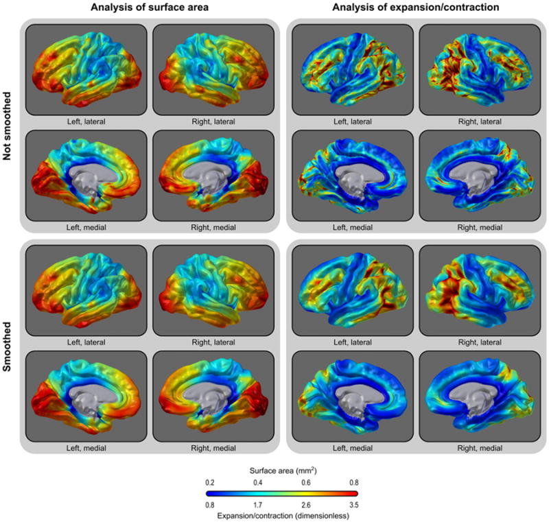
Average area (left panels) or expansion/contraction (right panels) per vertex, without (upper panels) and with smoothing (lower panels). Areal analyses and expansion/contraction differ across space. Smoothing has little global impact.

Fig. 9.

(a) The sum of the area per vertex correlates well with the average across space of the expansion/contraction at each vertex (i.e. equivalent to a weighed sum considering each vertex as having the same initial area) for the 168 hemispheres analyzed. For the expansion/contraction, this is not the same as computing the ratio between the global surface area in native geometry and of the template, in which case, the result would be a perfectly straight line. The high correlation implies that the regional differences in general compensate each other to produce a similar global effect. (b) The correlation between average spatial maps across the 84 subjects, both hemispheres, is very poor between the methods. [Note that, for (b), attempts to simultaneously plot all the > 300 thousand vertices would not produce meaningful plots in a small space; for this reason only 5% of the vertices were randomly selected for plotting. The R² were computed from all vertices and, for both (a) and (b), the value corresponds to the goodness of a linear fit.].

Fig. 10.

For each isolated vertex, the linear relationship between areal analyses and expansion/contraction is very high across subjects, being above R² = 0.90 virtually across the whole cortex.

These results suggest that, if each vertex is analyzed in isolation, analysis of surface area and analysis of expansion/contraction tend to produce similar results. This is the case, for instance, using mass univariate GLM-based approaches. However, for analysis that involve spatial information or that combine information across neighboring vertices, the results are expected to be rather dissimilar. The difference stems from the different units of measurement: areal analyses produce measurements in absolute units of area (e.g. mm²), whereas expansion/contraction is relative to the given reference. The result shown in Fig. 10, left panel, also demonstrates, indirectly, that areas measured in the retessellated brain with the resolution used correlate reasonably well with the areas obtained using areal interpolation, and so, have potential to be used as a fast approximation to areal interpolation (Appendix B). Conversely, expansion/contraction measurements can be obtained after areal interpolation simply by dividing the area per face (or per vertex) by its homologous in the reference brain.

Validation and stability

Measurements of surface area are valid as long as the surface reconstruction from MR images produces accurate representations of the cortex. The suggested reconstruction method has been previously validated (Fischl and Dale, 2000), and is widely used for cortical thickness measurements. Comparison between subjects at the face level depends on good matchingof homologies and the registration method we suggest has, likewise, been previously validated (Klein et al., 2010; Yeo et al., 2010a). As methods evolve, novel approaches for constructing surface representations of the cortex and for registration have potential to improve the overall quality of areal analyses. The validity of areal measurements other than surface area itself depends on each particular measurement technique.

To assess the stability across sessions and scanners, we compared MR images of the same subject acquired in three different sessions collected within a 1 year interval. The imaging protocol varied in terms of acquisition parameters, as well as the number of images used for averaging and improvements on signal and contrast-to-noise ratio. The details are summarized in Table 2. The estimated surface area produced by summing the facewise areas over the cortex after interpolation was very similar across tests, with the largest difference being 8.2% between Tests A and C (see Table 2), with or without smoothing. The mean and standard deviation for facewise areas were virtually identical across tests, again regardless of smoothing. The pairwise Pearson correlation between the tests for the facewise data after registration and interpolation was above 0.80 without smoothing, and above 0.90 after smoothing with FWHM = 10 mm, showing that the procedure is robust at the face level, even under different scanning conditions and degrees of smoothing.

Table 2.

Stability and robustness of measurements after registration and interpolation were assessed using three test images of the same subject. The measurements were similar across tests, with similar variability across space and high spatial correlation.

	Test A	Test B	Test C
Manufacturer and model	Siemens MAGNETOM Trio 3 T	Siemens MAGNETOM Trio/TIM 3 T	Siemens MAGNETOM Allegra 3 T
Sequence	MPRAGE	MPRAGE	MPRAGE
TE/TI/TR (ms)	3.04/785/2100	2.83/766/2200	2.74/900/2500
Flip angle	13°	13°	8°
Voxel size (mm)	0.8×0.8×0.8	0.8×0.8×0.8	1.0×1.0×1.0
Number of acquisitions	14	7	1
Scan date	March 2008	March 2008	April 2009
Cortical surface area (mm2)	176,996	177,098	180,949
Not smoothed
Average area per face (mm2)	0.2937	0.2939	0.3003
Standard deviation	0.0938	0.0910	0.0962
Correlation with Test A	–	0.8218	0.7589
Correlation with Test B	0.8218	–	0.7863
Correlation with Test C	0.7589	0.7863	–
Smoothed (FWHM = 10 mm)
Average area per face (mm2)	0.2935	0.2936	0.3000
Standard deviation	0.0746	0.0712	0.0748
Correlation with Test A	–	0.9509	0.9074
Correlation with Test B	0.9509	–	0.9353
Correlation with Test C	0.9047	0.9353	–

Discussion

Registration

To be valid, facewise analyses rely on the assumption that microscopic structures can be localized using as reference the features that are identifiable with MRI and which drive the registration. Features with such localizing power are important because they help to ensure good overlapofhomologousareas between subjects. Despiteanimplicit assumption already present in most imaging studies, only recently it has been demonstrated valid for some cytoarchitetonic areas when the references are the cortical folding patterns, even though for non-primary regions, the mismatch may still be substantial (Da Costa et al., 2011; Fischl et al., 2008, 2009; Hinds et al., 2008, 2009). Other features, some microscopic and detectable only under ultra-high field strengths (Augustinack et al., 2005; Bridge and Clare, 2006; Duyn et al., 2007; Kim et al., 2009), have the potential to be used as the reference as long as they are demonstrated to be markers of histologically or functionally defined areas, possibly replacing folding patterns altogether, or used to provide ancillary information. Myeloarchitectural features may be particularly useful for this application, for being responsible for most of the contrast observed with MRI (Geyer et al., 2011). Likewise, areal analyses can be conducted after registration based on features derived from functional MRI (Sabuncu et al., 2010).

Good matching of homologies, however, depends not only on the features used to guide the registration, but also on the registration method itself. For facewise areal analyses, invertibility is necessary to prevent faces from being folded over others. In addition, methods that produce smooth warps are necessary to ensure that areal quantities are transferred smoothly, without abrupt variations. Such abrupt variations would only be acceptable if matching perfectly with areas where structure and/or function also changes abruptly. A spatial transformation that allows such perfect matching, however, cannot be obtained easily in practice, since these borders usually cannot be observed with current, conventional MRI methods, and importantly, since many of the differences between regions are subtle and the transitions are gradual. However, invertibility and smoothness, as guaranteed by diffeomorphic methods, albeit important, may not suffice. Our results show that even methods that produce smooth varying warps can differ substantially with respect to how the areal quantities are shifted across the surface. It is possible that performance differences between these methods might be due to choices on regularization strategies and associated parameters (Fischl et al., 1999b; Yeo et al., 2010a), instigating further research on selections that may produce the most accurate results (Yeo et al., 2010b). Our experiments also demonstrate that the choice of the target used for registration affects the distortion in areal measurements.

Areal interpolation

Areal interpolation allows direct analysis of areal quantities in absolute values, including the surface area itself. This is because it is the areal quantity proper that is conservatively transferred between grids. Therefore, there is no need to apply corrections due to stretches or shrinkages, such as using the Jacobian of the transformation (Good et al., 2001), nor due to the choice of the parametrizable surface (Thompson and Toga, 1999). Moreover, the results are interpretable directly with regard to the actual amount of tissue or other measurement under study, rather than relative to concepts as expansion/contraction, which are always relative to a given reference, and can create difficulties in interpretation and comparison across studies, either due to different definitions adopted by different authors, or due to the need of a reference brain. Notwithstanding, after areal interpolation, it continues to be possible to divide the areas by the areas of the homologous faces or vertices of a reference brain, and so, obtain an expansion/contraction measurement. Moreover, areal quantities that are not area itself can also be divided by the area of each face or vertex in native geometry, thus converting these quantities to densities if necessary.

It should be emphasized that, as with other interpolation strategies, areal interpolation is not perfectly reversible, i.e. once the cortical area of a subject is transferred to a different grid, remapping back to the subject surface will not produce locally identical results, although the global areal quantity is always conserved. This is because within each face, the areal quantity is implicitly assumed to be homogeneously distributed. This only becomes a problem if low resolution meshes are used and if several back-and-forth iterations are performed.

Statistical analysis of areal quantities

There are a number of reasons that go beyond purely methodological considerations to justify the transformation of the data before statistical analysis. Measurements related to biological morphology, such as lengths, areas, volumes or weights, are well known to follow non-normal distributions. If the diameter of a structure, for instance, is normally distributed, inevitably both its cross section and its surface area follow skewed distributions, whereas its volume follows an even more skewed (Gaddum, 1945; Kapteyn and van Uven, 1916). All these related measurements cannot be normally distributed simultaneously. The skewness is higher when the variability is relatively large in comparison to the measure of central tendency that best describes the data, such as the arithmetic or the geometric mean. If the non-normality is not considered, statistical models are likely to produce inaccurate results. In this scenario, a power transformation, such as the Box–Cox transformation, helps to identify subjacent, possibly causative, normally distributed effects.

The lognormal distribution, more specifically, is known to arise in a variety of biological processes. Of particular interest is the autocatalytic growth of tissue over time. The number of cells present on a tissue that grows in an unrestricted way can be given by the familiar formula N = N₀e^ct, where N₀ is the initial number of cells, and t is the amount of time in which the cell grows under the circumstances represented by the constant c, a factor that incorporates a variety of influences, such as genetic and environmental. N will be lognormally distributed if either c or t are normally distributed (Koch, 1966; Limpert et al., 2001). The finding that the facewise cortical surface area follows mostly lognormal distributions may suggest that the method may capture these biological effects. Such interpretation can only subsist under the tenets of accurate and smooth registration.

From a statistical perspective, permutation methods do not rely on normality, rendering them appropriate in a variety of situations in which this assumption is not tenable. Nevertheless, the data should, still, undergo a transformation. As discussed above, the reason is not merely to conform to normality, although that comes as a bonus, but also to ensure that underlying biological effects, either multiplicative or proportionally dependent upon an initial value, can be treated as additive in a linear model (Christensen, 2002). Areal quantities that are not the cortical surface area itself can, notwithstanding, be distributed differently, and the framework for statistical analysis outlined in the Methods section appears generic enough to accommodate a variety cases. The Box–Cox transformation has yet another advantage when used in combination with permutation methods under multiple testing conditions: the more stable variance after the transformation allows the distribution of the statistic under null hypothesis to become more similar across tests, allowing FWER to be controlled at a level closer to its nominal value using the distribution of the maximum statistic.

Further developments and potential applications

Facewise analyses offer the possibility of studying surface area at a much finer scale than previously. This is a feature of interest in many research fields across the neurosciences, as well as in medicine. Although the same applies to vertexwise cortical thickness, thickness and area provide different and complementary insights into processes underlying the development of the brain and disorders (Sanabria-Diaz et al., 2010; Voets et al., 2008; Winkler et al., 2010).

Provided that the neurons in the cortex retain largely their same relative positions as the progenitor cells in the embryo (Clowry et al., 2010; Pierani and Wassef, 2009; Rakic, 1988, 2009), facewise comparison of surface area allows one to hypothesize about ontogenetic processes to the extent that they can be observed and localized with MRI, even long after the end of phases of massive tangential cellular proliferation. Until now, this kind of study could not be performed, either due to lack of methods to analyze cortical surface area without the constrains imposed by regions of interest, or due to inherent limitations of methods based on expansion or contraction.

The study of local cortical surface area offers, moreover, new possibilities for connectivity analyses, as the need for parcellations based on macroscopic anatomy is obviated. Indeed, the results of connectivity analyses are known to be influenced by the choice of the parcellation that define nodes of putative neuronal networks (Butts, 2009; Rubinov and Sporns, 2010). Notwithstanding, if a given set of regions is derived from a different method (Beckmann et al., 2009; Nelson et al., 2010), these can be directly associated with their corresponding surface-based areas or areal quantities by means of areal interpolation.

Another potential application is for genetic analyses. Given that cortical surface area and thickness are both heritable, yet genetically not correlated (Panizzon et al., 2009; Winkler et al., 2010), these traits, separately, can be used in a framework similar to voxelwise genome-wide association studies (vGWAS) (Stein et al., 2010). Identification of genes that influence surface area has potential to elucidate a myriad of developmental, neurologic and psychiatric disorders.

Conclusion

We presented an interpolation method for between-subject analyses of cortical surface area. The method is also suitable for other quantities that are areal by nature and which require mass conservation (pycnophylactic property) during interpolation and analysis. We demonstrated that, when the quantity under study is surface area itself, the distribution of the data does not follow a normal distribution, being instead better characterized as lognormal, and proposed a framework for statistical analysis and inference. An Octave/MATLAB implementation of areal interpolation is available from the authors at http://brainder.org.

Supplementary materials related to this article can be found online at doi:10.1016/j.neuroimage.2012.03.026.

Appendix A. Geodesic spheres and areal inequalities

The only required feature for the common grid used for the areal interpolation is that all its vertices must lie on the surface of a sphere. The algorithm we present in Appendix B requires further that all faces of the sphere are triangular and that all edges of all faces are much smaller than the radius, so that areal distortion is minimized when projecting to a plane.

A common grid that meet these demands is a sufficiently fine geodesic sphere. There are different ways to construct such a sphere (Kenner, 1976). One method is to subdivide each face of a regular polyhedron with triangular faces, such as the icosahedron, into four new triangles. The new vertices are projected to the surface of the (virtual) circumscribed sphere along its radius and the process is repeated recursively a number of times (Lauchner et al., 1969). For the n-th iteration, the number of faces is given by F = 4ⁿF₀, the number of vertices by V = 4ⁿ(V₀ − 2) + 2, and the number of edges by E = 4ⁿE₀, where F₀, V₀ and E₀ are, respectively, the number of faces, vertices and edges of the polyhedron with triangular faces used for the initial subdivision. For the icosahedron, F₀ = 20, V₀ = 12 and E₀ = 30 (Fig. 11a). For the analyses in this manuscript, we used n = 7, producing geodesic spheres with 327680 faces and 163842 vertices.

Fig. 11.

(a) The common grid can be a geodesic sphere produced from recursive subdivision of a regular icosahedron. At each iteration, the number of faces is quadrupled. (b) After the first iteration, however, the faces no longer have regular sizes, with the largest face being approximately 1.3 times larger than the smallest as n increases.

These faces, however, do not have identical edge lengths and areas (Kenner, 1976), even though the initial icosahedron was perfectly regular. This is important for areal interpolation, as larger faces on the target grid do overlap with more faces from the source surfaces, absorbing larger amounts of areal quantities, possibly causing confusion if one attempts to color-encode the interpolated image according to the actual areal quantities, in which case, geometric patterns such as in Fig. 11b will become evident. Moreover, smoothing can cause quantities that are arbitrarily large or small due to face sizes to be blurred into the neighbors. Both potential problems can be addressed by multiplying the areal quantity at each face j, after interpolation, by a constant given by $4\pi r^2/\left(A_j^{T}F\right)$, where $A_j^T$ is the area of the same face of the geodesic sphere, F is the number of faces, and r is the radius of the sphere.

Appendix B. Implementation

The areal interpolation for spheres is implemented in two parts. In the first, we compute inside of which source faces the target vertices are located, creating a lookup table to be used in the second part. This is the point-in-polygon problem found in vector graphics applications (Vince, 2005). Here we calculate the area of each source face, $A_i^S$, and the subsequent steps proceed iteratively for each face in the source. The barycentric coordinates of each candidate vertex in relation to the current face i is computed; if their sum equals to unity, the point is labeled as inside. However, to test if all vertices are inside every face would needlessly waste computational time. Moreover, since all points are on the surface of a sphere, the vertices in the target are never expected to be coplanar to the source triangular faces, so the test would always fail. The first problem is treated by testing only the vertices located within a bounding box defined, still in the 3D space, from the source face extreme coordinates. The second could naïvely be treated by converting the 3D Cartesian coordinates to 2D spherical coordinates, which allow a fast flattening of the sphere to the popular plate carrée cylindrical projection. However, latitude is ill-defined at the poles in cylindrical projections. Moreover, cylindrical projections introduce a specific type of deformation that is undesired here: straight lines on the surface (geodesic lines) are distorted. The solution we adopt is to rotate the Cartesian coordinate system so that the barycenter of the current source face lies at the point (r, 0, 0), where r is the radius of the source and target spheres. The barycenter is used for ease of calculation and for being always inside the triangle. After rotation, the current face and the nearby candidate target vertices are projected to a plane using the azimuthal gnomonic projection (Snyder, 1987), centered at the barycenter of the face. The point-in-polygon test can then be applied successfully. The key advantage of the gnomonic projection is that all geodesics project as straight lines, rather than loxodromic or other complex paths as with other projections, which would cause many target vertices to be incorrectly labeled. This projection can be obtained trivially after the rotation of the 3D Cartesian coordinate system as φ = y/x and θ = z/x, where (x, y, z) are the 3D coordinates of the point being projected. A potential disadvantage of the gnomonic projection is the remarkable areal distortion for regions distant from the center of the projection. Since in typical neuroimaging applications the source and target spheres are composed of a tessellation of approximately 3 × 10⁶ faces, $A_i^S\ll 4\pi r^2$, and the distortion becomes negligible.

In the second part, the areal interpolation is performed, with the overlapping areas being calculated and used to weigh the areal quantity under study. The identification of intersections between two sets of polygons is also a well studied problem in vector graphics (Chazelle et al., 1994; Guibas and Seidel, 1987), which solution depends on optimally finding crossings between multiple line segments (Balaban, 1995; Bentley and Ottmann, 1979; Chazelle and Edelsbrunner, 1992). Most of the efficient available algorithms assume that the polygons are all coplanar; those that work in the surface of a sphere use coordinates expressed in latitude and longitude and require special treatment of the polar regions. The solution we adopt obviates these problems by first computing the area of each target face, $A_j^T$; the subsequent steps are performed iteratively for each face in the target sphere, using the azimuthal gnomonic projection, similarly as in the first part, but now centered at the barycenter of the current target face at every iteration. The areal quantities assigned to the faces in the target sphere are initialized as zero before the loop begins. If all three vertices of the current target face j lie inside the same source face k, as known from the lookup table produced in the first part, then to the current face the areal quantity given by $Q_j^T=Q_k^S{A}_j^T/A_k^S$ is assigned. Otherwise, the source faces that surround the target are examined to find overlaps. This is done by considering the edges of the current target face as vectors organized in counter-clockwise orientation, and testing if the vertices of the candidate faces lie on the left, right or if they coincide with the edge. If all the three vertices of any candidate face are on the right of any edge, there is no overlap and the candidate face is removed from further consideration. If all the three vertices are on the left of all three edges, then the candidate source face is entirely inside the target, which has then its areal quantity incremented as $Q_j^T\leftarrow Q_j^T+Q_k^S$. The remaining faces are those that contain some vertices on the left and some on the right of the edges of the current, target face. The intersections between these source and target edges are computed and false intersections between edge extensions are ignored. A list containing the vertices for each candidate source face that are inside the target face (known for being on the left of the three target edges), the target vertices that are inside each of the source faces (known from the lookup table) and the coordinates of the intersections between face edges, is used to compute the convex hull, using the Quickhull algorithm (Barber et al., 1996). The convex hull delimits the overlapping region between the current target face j and the candidate source face k, which area, $A_k^O$, is used to increment the areal quantity assigned to the target face as $Q_j^T\leftarrow Q_j^T+Q_k^S{A}_k^O/A_k^S$.

The algorithm runs in O(n) for n faces, as opposed to O(n²) that would be obtained by naïve search. Nevertheless, the current implementation in Octave/MATLAB, a dynamically typed, interpreted language, requires about 24 hours to run in a computer with 2.66 GHz Intel Xeon processors.

Appendix C. Conversion from facewise to vertexwise

Whenever it is necessary to perform analyses that include measurements taken at each vertex (such as some areal quantity versus cortical thickness) or when only software that can display vertexwise data is available (Appendix D), it may be necessary to convert the areal quantities from facewise to vertexwise. The conversion can be done by redistributing the quantities at each face to their three constituent vertices. The areal values assigned to the faces that meet at a given vertex are summed, and divided by three, and reassigned to this vertex. Importantly, this procedure has to be done after the areal interpolation, since interpolation methods for vertexwise data are not appropriate for areal quantities, and before the statistical analysis, since the average of the results of the statistics of a test is not necessarily the same as the statistic for the average of the original data. It should also be observed that conversion from facewise to vertexwise data implies a loss of resolution to approximately half of the original and, therefore, should be performed only if resolution is not a concern and there is no other way to analyze, visualize, or present facewise data or results. The conversion does not change the underlying distribution, provided that the resolution of the initial mesh is sufficiently fine.

Appendix D. Presentation of results

To display results, facewise data can be projected from the common grid to the template geometry, which helps to visually identify anatomical landmarks and name structures. Projecting data from one surface to another is trivial as there is a one-to-one mapping between faces of the grid and the template geometry. The statistics and associated p-values can be encoded in colors, and a color scale can be shown along with the surface model.

However, the presentation of facewise data has conceptual differences in comparison with the presentation vertexwise data. For vertexwise data, each vertex cannot be directly colored, for being dimensionless. Instead, to display data per vertex, typically each face has its color interpolated according to the colors of its three defining vertices, forming a linear gradient that covers the whole face. For facewise data there is no need to perform such interpolation of colors, since the faces can be shown directly on the 3D space, each one in the uniform color that represents the underlying data. The difference is shown in Fig. 12.

Fig. 12.

Differences between presentation of facewise and vertexwise data can be observed in this zoomed portion of the mesh representation of the cortex. Vertices are dimensionless and, to display vertexwise data, the faces have to be colored using linear interpolation. This is not necessary for facewise data, which can be shown directly in the uniform colors that represent the underlying data. In either case, the presentation can be improved by using a shading model, such as Gouraud in this example. Although the vertexwise presentation may be visually more appealing, it contains only half the resolution of the facewise image.

Interpolation of colors for vertexwise data should not be confused with the related, yet different concept of lightning and shading using interpolation. Both vertexwise and facewise data can be shaded to produce more realistic images. In Fig. 12 we give an example of simple flat shading and shading based on linear interpolation of the lightning at each vertex (Gouraud, 1971).

Currently available software allow the presentation of color-encoded vertexwise data on the surface of meshes. However, only very few software applications can handle a large number of colors per 3D object, being one color per face. One example is Blender (Blender Foundation, Amsterdam, The Netherlands), which we used to produce the figures presented in this article. Another option, for instance, is to use low-level mesh commands in MATLAB, such as patch.

References

- Augustinack JC, van der Kouwe AJ, Blackwell ML, Salat DH, Wiggins CJ, Frosch MP, Wiggins CC, Potthast A, Wald LL, Fischl BR. Detection of entorhinal layer II using 7 Tesla magnetic resonance imaging. Ann Neurol. 2005;57(4):489–494. doi: 10.1002/ana.20426. [DOI] [PMC free article] [PubMed] [Google Scholar]
- Balaban IJ. An optimal algorithm for finding segments intersections. Proceedings of the 11th Annual Symposium on Computational Geometry. 1995:211–219. [Google Scholar]
- Barber CB, Dobkin DP, Huhdanpaa HT. The Quickhull algorithm for convex hulls. ACM Trans Math Softw. 1996;22(4):469–483. [Google Scholar]
- Beckmann M, Johansen-Berg H, Rushworth MFS. Connectivity-based parcellation of human cingulate cortex and its relation to functional specialization. J Neurosci. 2009;29(4):1175–1190. doi: 10.1523/JNEUROSCI.3328-08.2009. [DOI] [PMC free article] [PubMed] [Google Scholar]
- Benjamini Y, Hochberg Y. Controlling the false discovery rate: a practical and powerful approach to multiple testing. J R Stat Soc Ser B. 1995;57(1):289–300. [Google Scholar]
- Bentley JL, Ottmann TA. Algorithms for reporting and counting geometric intersections. IEEE Trans Comput. 1979;C-28(9):643–647. [Google Scholar]
- Bilgüvar K, Oztürk AK, Louvi A, Kwan KY, Choi M, Tatli B, Yalnizo lu D, Tüysüz B, Ca layan AO, Gökben S, Kaymakćalan H, Barak T, Bakircio lu M, Yasuno K, Ho W, Sanders S, Zhu Y, Yilmaz S, Dinçer A, Johnson MH, Bronen RA, Koçer N, Per H, Mane S, Pamir MN, Yalçinkaya C, Kumanda S, Topçu M, Ozmen M, Sestan N, Lifton RP, State MW, Günel M. Whole-exome sequencing identifies recessive WDR62 mutations in severe brain malformations. Nature. 2010;467(7312):207–210. doi: 10.1038/nature09327. [DOI] [PMC free article] [PubMed] [Google Scholar]
- Box G, Cox D. An analysis of transformations. J R Stat Soc Ser B. 1964;26(2):211–252. [Google Scholar]
- Bridge H, Clare S. High-resolution MRI: in vivo histology? Phil Trans R Soc B. 2006;361(1465):137–146. doi: 10.1098/rstb.2005.1777. [DOI] [PMC free article] [PubMed] [Google Scholar]
- Butts CT. Revisiting the foundations of network analysis. Science. 2009;325(5939):414–416. doi: 10.1126/science.1171022. [DOI] [PubMed] [Google Scholar]
- Buxhoeveden DP, Casanova MF. The minicolumn hypothesis in neuroscience. Brain. 2002;125(5):935–951. doi: 10.1093/brain/awf110. [DOI] [PubMed] [Google Scholar]
- Chazelle B, Edelsbrunner H. An optimal algorithm for intersecting line segments in the plane. J ACM. 1992;39(1):1–54. [Google Scholar]
- Chazelle B, Edelsbrunner H, Guibas LJ, Sharir M. Algorithms for bichromatic line-segment problems and polyhedral terrains. Algorithmica. 1994;11(2):116–132. [Google Scholar]
- Chen CH, Panizzon M, Eyler L, Jernigan T, Thompson W, Fennema-Notestine C, Jak A, Neale M, Franz C, Hamza S, Lyons M, Grant M, Fischl B, Seidman L, Tsuang M, Kremen W, Dale A. Genetic influences on cortical regionalization in the human brain. Neuron. 2011;72(4):537–544. doi: 10.1016/j.neuron.2011.08.021. [DOI] [PMC free article] [PubMed] [Google Scholar]
- Chenn A, Walsh CA. Regulation of cerebral cortical size by control of cell cycle exit in neural precursors. Science. 2002;297(5580):365–369. doi: 10.1126/science.1074192. [DOI] [PubMed] [Google Scholar]
- Christensen R. Plane answers to complex questions: the theory of linear models. Springer; New York: 2002. [Google Scholar]
- Christensen GE, Rabbitt RD, Miller MI. Deformable templates using large deformation kinematics. IEEE Trans Image Process. 1996;5(10):1435–1447. doi: 10.1109/83.536892. [DOI] [PubMed] [Google Scholar]
- Clark CM, Schneider JA, Bedell BJ, Beach TG, Bilker WB, Mintun MA, Pontecorvo MJ, Hefti F, Carpenter AP, Flitter ML, Krautkramer MJ, Kung HF, Coleman RE, Doraiswamy PM, Fleisher AS, Sabbagh MN, Sadowsky CH, Reiman EP, Reiman PEM, Zehntner SP, Skovronsky DM. Use of florbetapir-PET for imaging beta-amyloid pathology. JAMA. 2011;305(3):275–283. doi: 10.1001/jama.2010.2008. [DOI] [PMC free article] [PubMed] [Google Scholar]
- Clowry G, Molnár Z, Rakic P. Renewed focus on the developing human neocortex. J Anat. 2010;217(4):276–288. doi: 10.1111/j.1469-7580.2010.01281.x. [DOI] [PMC free article] [PubMed] [Google Scholar]
- Da Costa S, van der Zwaag W, Marques JP, Frackowiak RSJ, Clarke S, Saenz M. Human primary auditory cortex follows the shape of Heschl's gyrus. J Neurosci. 2011;31(40):14067–14075. doi: 10.1523/JNEUROSCI.2000-11.2011. [DOI] [PMC free article] [PubMed] [Google Scholar]
- Dale AM, Sereno MI. Improved localization of cortical activity by combining EEG and MEG with MRI cortical surface reconstruction. J Cogn Neurosci. 1993;5(2):162–176. doi: 10.1162/jocn.1993.5.2.162. [DOI] [PubMed] [Google Scholar]
- Dale AM, Fischl B, Sereno MI. Cortical surface-based analysis I: segmentation and surface reconstruction. NeuroImage. 1999;9(2):179–194. doi: 10.1006/nimg.1998.0395. [DOI] [PubMed] [Google Scholar]
- De Boor C. Bicubic spline interpolation. J Math Phys. 1962;41(3):212–218. [Google Scholar]
- Desikan RS, Ségonne F, Fischl B, Quinn BT, Dickerson BC, Blacker D, Buckner RL, Dale AM, Maguire RP, Hyman BT, Albert MS, Killiany RJ. An automated labeling system for subdividing the human cerebral cortex on MRI scans into gyral based regions of interest. NeuroImage. 2006;31:968–980. doi: 10.1016/j.neuroimage.2006.01.021. [DOI] [PubMed] [Google Scholar]
- Dickerson BC, Feczko E, Augustinack JC, Pacheco J, Morris JC, Fischl B, Buckner RL. Differential effects of aging and Alzheimer's disease on medial temporal lobe cortical thickness and surface area. Neurobiol Aging. 2009;30(3):432–440. doi: 10.1016/j.neurobiolaging.2007.07.022. [DOI] [PMC free article] [PubMed] [Google Scholar]
- Drury HA, Van Essen DC, Anderson CH, Lee CW, Coogan TA, Lewis JW. Computerized mappings of the cerebral cortex: a multiresolution flattening method and a surface-based coordinate system. J Cogn Neurosci. 1996;8(1):1–28. doi: 10.1162/jocn.1996.8.1.1. [DOI] [PubMed] [Google Scholar]
- Durazzo TC, Tosun D, Buckley S, Gazdzinski S, Mon A, Fryer SL, Meyerhoff DJ. Cortical thickness, surface area, and volume of the brain reward system in alcohol dependence: relationships to relapse and extended abstinence. Alcohol Clin Exp Res. 2011;35(6):1–14. doi: 10.1111/j.1530-0277.2011.01452.x. [DOI] [PMC free article] [PubMed] [Google Scholar]
- Duyn JH, van Gelderen P, Li TQ, de Zwart JA, Koretsky AP, Fukunaga M. High-field MRI of brain cortical substructure based on signal phase. Proc Natl Acad Sci U S A. 2007;104(28):11796–11801. doi: 10.1073/pnas.0610821104. [DOI] [PMC free article] [PubMed] [Google Scholar]
- Eyler LT, Prom-Wormley E, Panizzon MS, Kaup AR, Fennema-Notestine C, Neale MC, Jernigan TL, Fischl B, Franz CE, Lyons MJ, Grant M, Stevens A, Pacheco J, Perry ME, Schmitt JE, Seidman LJ, Thermenos HW, Tsuang MT, Chen CH, Thompson WK, Jak A, Dale AM, Kremen WS. Genetic and environmental contributions to regional cortical surface area in humans: a magnetic resonance imaging twin study. Cereb Cortex. 2011;21(10):2313–2321. doi: 10.1093/cercor/bhr013. [DOI] [PMC free article] [PubMed] [Google Scholar]
- Fischl B, Dale AM. Measuring the thickness of the human cerebral cortex from magnetic resonance images. Proc Natl Acad Sci U S A. 2000;97(20):11050–11055. doi: 10.1073/pnas.200033797. [DOI] [PMC free article] [PubMed] [Google Scholar]
- Fischl B, Sereno MI, Dale AM. Cortical surface-based analysis II: Inflation, flattening, and a surface-based coordinate system. NeuroImage. 1999a;9(2):195–207. doi: 10.1006/nimg.1998.0396. [DOI] [PubMed] [Google Scholar]
- Fischl B, Sereno MI, Tootell RB, Dale AM. High-resolution intersubject averaging and a coordinate system for the cortical surface. Hum Brain Mapp. 1999b;8(4):272–284. doi: 10.1002/(SICI)1097-0193(1999)8:4<272::AID-HBM10>3.0.CO;2-4. [DOI] [PMC free article] [PubMed] [Google Scholar]
- Fischl B, Liu A, Dale AM. Automated manifold surgery: constructing geometrically accurate and topologically correct models of the human cerebral cortex. IEEE Trans Med Imaging. 2001;20(1):70–80. doi: 10.1109/42.906426. [DOI] [PubMed] [Google Scholar]
- Fischl B, Rajendran N, Busa E, Augustinack J, Hinds O, Yeo BT, Mohlberg H, Amunts K, Zilles K. Cortical folding patterns and predicting cytoarchitecture. Cereb Cortex. 2008;18(8):1973–1980. doi: 10.1093/cercor/bhm225. [DOI] [PMC free article] [PubMed] [Google Scholar]
- Fischl B, Stevens AA, Rajendran N, Yeo BT, Greve DN, Leemput KV, Polimeni JR, Kakunoori S, Buckner RL, Pacheco J, Salat DH, Melcher J, Frosch MP, Hyman BT, Grant PE, Rosen BR, van der Kouwe AJ, Wiggins GC, Wald LL, Augustinack JC. Predicting the location of entorhinal cortex from MRI. NeuroImage. 2009;47(1):8–17. doi: 10.1016/j.neuroimage.2009.04.033. [DOI] [PMC free article] [PubMed] [Google Scholar]
- Fish JL, Dehay C, Kennedy H, Huttner WB. Making bigger brains—the evolution of neural-progenitor-cell division. J Cell Sci. 2008;121:2783–2793. doi: 10.1242/jcs.023465. [DOI] [PubMed] [Google Scholar]
- Flowerdew R, Green M, Kehris E. Using areal interpolation methods in geographic information systems. Pap Reg Sci. 1991;70(3):303–315. [Google Scholar]
- Gaddum JH. Lognormal distributions. Nature. 1945;156(3964):463–466. [Google Scholar]
- Genovese CR, Lazar NA, Nichols T. Thresholding of statistical maps in functional neuroimaging using the false discovery rate. NeuroImage. 2002;15(4):870–878. doi: 10.1006/nimg.2001.1037. [DOI] [PubMed] [Google Scholar]
- Geyer S, Weiss M, Reimann K, Lohmann G, Turner R. Microstructural parcellation of the human cerebral cortex—from Brodmann's post-mortem map to in vivo mapping with high-field magnetic resonance imaging. Front Hum Neurosci. 2011;5:19. doi: 10.3389/fnhum.2011.00019. [DOI] [PMC free article] [PubMed] [Google Scholar]
- Glaunès J, Vaillant M, Miller MI. Landmark matching via large deformation diffeomorphisms on the sphere. J Math Imaging Vis. 2004;1–2:179–200. [Google Scholar]
- Good CD, Johnsrude IS, Ashburner J, Henson RN, Friston KJ, Frackowiak RS. A voxel-based morphometric study of ageing in 465 normal adult human brains. NeuroImage. 2001;14(1 Pt 1):21–36. doi: 10.1006/nimg.2001.0786. [DOI] [PubMed] [Google Scholar]
- Goodchild MF, Lam NSN. Areal interpolation: a variant of the traditional spatial problem. Geo-Processing. 1980;1:297–312. [Google Scholar]
- Gouraud H. Continuous shading of curved surfaces. 6. C-20. IEEE Trans Comput; 1971. pp. 623–629. [Google Scholar]
- Gregory IN, Marti-Henneberg J, Tapiador FJ. Modelling long-term pan-European population change from 1870 to 2000 by using geographical information systems. J Roy Statist Soc Ser A. 2010;173(1):31–50. [Google Scholar]
- Guibas LJ, Seidel R. Computing convolutions by reciprocal search. Discret Comput Geom. 1987;2(1):175–193. [Google Scholar]
- Hagler DJ, Saygin AP, Sereno MI. Smoothing and cluster thresholding for cortical surface-based group analysis of fMRI data. NeuroImage. 2006;33(4):1093–1103. doi: 10.1016/j.neuroimage.2006.07.036. [DOI] [PMC free article] [PubMed] [Google Scholar]
- Hill J, Inder T, Neil J, Dierker D, Harwell J, van Essen D. Similar patterns of cortical expansion during human development and evolution. Proc Natl Acad Sci U S A. 2010;107(29):13135–13140. doi: 10.1073/pnas.1001229107. [DOI] [PMC free article] [PubMed] [Google Scholar]
- Hinds OP, Rajendran N, Polimeni JR, Augustinack JC, Wiggins G, Wald LL, Rosas HD, Potthast A, Schwartz EL, Fischl B. Accurate prediction of V1 location from cortical folds in a surface coordinate system. NeuroImage. 2008;39(4):1585–1599. doi: 10.1016/j.neuroimage.2007.10.033. [DOI] [PMC free article] [PubMed] [Google Scholar]
- Hinds O, Polimeni JR, Rajendran N, Balasubramanian M, Amunts K, Zilles K, Schwartz EL, Fischl B, Triantafyllou C. Locating the functional and anatomical boundaries of human primary visual cortex. NeuroImage. 2009;46(4):915–922. doi: 10.1016/j.neuroimage.2009.03.036. [DOI] [PMC free article] [PubMed] [Google Scholar]
- Holmes AP, Blair RC, Watson JD, Ford I. Nonparametric analysis of statistic images from functional mapping experiments. J Cereb Blood Flow Metab. 1996;16(1):7–22. doi: 10.1097/00004647-199601000-00002. [DOI] [PubMed] [Google Scholar]
- Jones PW. First- and second-order conservative remapping schemes for grids in spherical coordinates. Mon Weather Rev. 1999;127(9):2204–2210. [Google Scholar]
- Jones EG. Microcolumns in the cerebral cortex. Proc Natl Acad Sci U S A. 2000;97(10):5019–5021. doi: 10.1073/pnas.97.10.5019. [DOI] [PMC free article] [PubMed] [Google Scholar]
- Joyner AH, Roddey JC, Bloss CS, Bakken TE, Rimol LM, Melle I, Agartz I, Djurovic S, Topol EJ, Schork NJ, Andreassen OA, Dale AM. A common MECP2 haplotype associates with reduced cortical surface area in humans in two independent populations. Proc Natl Acad Sci U S A. 2009;106(36):15483–15488. doi: 10.1073/pnas.0901866106. [DOI] [PMC free article] [PubMed] [Google Scholar]
- Kähler AK, Djurovic S, Rimol LM, Brown AA, Athanasiu L, Jönsson EG, Hansen T, Gústafsson O, Hall H, Giegling I, Muglia P, Cichon S, Rietschel M, Pietiläinen OP, Peltonen L, Bramon E, Collier D, Clair DS, Sigurdsson E, Petursson H, Rujescu D, Melle I, Werge T, Steen VM, Dale AM, Matthews RT, Agartz I, Andreassen OA. Candidate gene analysis of the human natural killer-1 carbohydrate pathway and perineuronal nets in schizophrenia: B3GAT2 is associated with disease risk and cortical surface area. Biol Psychiatry. 2011;69(1):90–96. doi: 10.1016/j.biopsych.2010.07.035. [DOI] [PubMed] [Google Scholar]
- Kapteyn JC, van Uven MJ. Skew Frequency Curves in Biology and Statistics. Hoitsema Brothers; Groningen, The Netherlands: 1916. [Google Scholar]
- Kenner H. Geodesic Math and How to Use It. University of California Press; Los Angeles, CA, USA: 1976. [Google Scholar]
- Kim JS, Singh V, Lee JK, Lerch J, Ad-Dab'bagh Y, MacDonald D, Lee JM, Kim SI, Evans AC. Automated 3-D extraction and evaluation of the inner and outer cortical surfaces using a Laplacian map and partial volume effect classification. NeuroImage. 2005;27(1):210–221. doi: 10.1016/j.neuroimage.2005.03.036. [DOI] [PubMed] [Google Scholar]
- Kim EY, Kim DH, Chang JH, Yoo E, Lee JW, Park HJ. Triple-layer appearance of Brodmann area 4 at thin-section double inversion-recovery MR imaging. Radiology. 2009;250(2):515–522. doi: 10.1148/radiol.2502080266. [DOI] [PubMed] [Google Scholar]
- Klein A, Ghosh SS, Avants B, Yeo BTT, Fischl B, Ardekani B, Gee JC, Mann JJ, Parsey RV. Evaluation of volume-based and surface-based brain image registration methods. NeuroImage. 2010;51(1):214–220. doi: 10.1016/j.neuroimage.2010.01.091. [DOI] [PMC free article] [PubMed] [Google Scholar]
- Klunk WE, Engler H, Nordberg A, Wang Y, Blomqvist G, Holt DP, Bergström M, Savitcheva I, Huang GF, Estrada S, Ausén B, Debnath ML, Barletta J, Price JC, Sandell J, Lopresti BJ, Wall A, Koivisto P, Antoni G, Mathis CA, Långström B. Imaging brain amyloid in Alzheimer's disease with Pittsburgh Compound-B. Ann Neurol. 2004;55(3):306–319. doi: 10.1002/ana.20009. [DOI] [PubMed] [Google Scholar]
- Koch AL. The logarithm in biology. 1. Mechanisms generating the log-normal distribution exactly. J Theor Biol. 1966;12(2):276–290. doi: 10.1016/0022-5193(66)90119-6. [DOI] [PubMed] [Google Scholar]
- Kochunov P, Lancaster JL, Glahn DC, Purdy D, Laird AR, Gao F, Fox PT. Retrospective motion correction protocol for high-resolution anatomical MRI. Hum Brain Mapp. 2006;27(12):957–962. doi: 10.1002/hbm.20235. [DOI] [PMC free article] [PubMed] [Google Scholar]
- Lauchner JH, Buckminster Fuller R, Clinton JD, Mabee MB, Moeller RM, Flood R. NASA contract NGR-14-008-002. Tech. rep., Southern Illinois University; 1969. Structural design concepts for future space missions. [Google Scholar]
- Lauritzen PH, Nair RD. Monotone and conservative cascade remapping between spherical grids (CaRS): regular latitude-longitude and cubed-sphere grids. Mon Weather Rev. 2008;136(4):1416–1432. [Google Scholar]
- Limpert E, Stahel Wa, Abbt M. Log-normal distributions across the sciences: keys and clues. BioScience. 2001;51(5):341–352. [Google Scholar]
- Lombardi M. Interpolation and smoothing. Astron Astrophys. 2002;395(2):733–745. [Google Scholar]
- Lyttelton OC, Karama S, Ad-Dab'bagh Y, Zatorre RJ, Carbonell F, Worsley K, Evans AC. Positional and surface area asymmetry of the human cerebral cortex. NeuroImage. 2009;46(4):895–903. doi: 10.1016/j.neuroimage.2009.03.063. [DOI] [PubMed] [Google Scholar]
- Mangin JF, Frouin V, Bloch I, Regis J, Lopes-Krabe J. From 3D MR images to structural representations of the cortex topography using topology preserving deformations. J Math Imaging Vis. 1995;5:297–318. [Google Scholar]
- Markoff J, Shapiro G. The linkage of data describing overlapping geographical units. Hist Meth Newslett. 1973;7(1):34–46. [Google Scholar]
- Miller M, Banerjeea A, Christensen G, Joshi S, Khaneja N, Grenander U, Matejic L. Statistical methods in computational anatomy. Stat Methods Med Res. 1997;6(3):267–299. doi: 10.1177/096228029700600305. [DOI] [PubMed] [Google Scholar]
- Mountcastle VP. Perceptual Neuroscience: The Cerebral Cortex. Harvard University Press; Cambridge, MA, USA: 1998. [Google Scholar]
- Nelson SM, Cohen AL, Power JD, Wig GS, Miezin FM, Wheeler ME, Velanova K, Donaldson DI, Phillips JS, Schlaggar BL, Petersen SE. A parcellation scheme for human left lateral parietal cortex. Neuron. 2010;67(1):156–170. doi: 10.1016/j.neuron.2010.05.025. [DOI] [PMC free article] [PubMed] [Google Scholar]
- Nichols T, Hayasaka S. Controlling the familywise error rate in functional neuroimaging: a comparative review. Stat Methods Med Res. 2003;12(5):419–446. doi: 10.1191/0962280203sm341ra. [DOI] [PubMed] [Google Scholar]
- Nopoulos PC, Aylward EH, Ross CA, Johnson HJ, Magnotta VA, Juhl AR, Pierson RK, Mills J, Langbehn DR, Paulsen JS PREDICT-HD Investigators Coordinators of Huntington Study Group (HSG) Cerebral cortex structure in prodromal Huntington disease. Neurobiol Dis. 2010;40(3):544–554. doi: 10.1016/j.nbd.2010.07.014. [DOI] [PMC free article] [PubMed] [Google Scholar]
- Palaniyappan L, Mallikarjun P, Joseph V, White TP, Liddle PF. Regional contraction of brain surface area involves three large-scale networks in schizophrenia. Schizophr Res. 2011;129(2–3):163–168. doi: 10.1016/j.schres.2011.03.020. [DOI] [PubMed] [Google Scholar]
- Panizzon MS, Fennema-Notestine C, Eyler LT, Jernigan TL, Prom-Wormley E, Neale M, Jacobson K, Lyons MJ, Grant MD, Franz CE, Xian H, Tsuang M, Fischl B, Seidman L, Dale A, Kremen WS. Distinct genetic influences on cortical surface area and cortical thickness. Cereb Cortex. 2009;19(11):2728–2735. doi: 10.1093/cercor/bhp026. [DOI] [PMC free article] [PubMed] [Google Scholar]
- Pierani A, Wassef M. Cerebral cortex development: from progenitors to patterning to neocortical size during evolution. Dev Growth Differ. 2009;51:325–342. doi: 10.1111/j.1440-169X.2009.01095.x. [DOI] [PubMed] [Google Scholar]
- Rakic P. Specification of cerebral cortical areas. Science. 1988;241(4862):170–176. doi: 10.1126/science.3291116. [DOI] [PubMed] [Google Scholar]
- Rakic P. Evolution of the neocortex: a perspective from developmental biology. Nat Rev Neurosci. 2009;10(10):724–735. doi: 10.1038/nrn2719. [DOI] [PMC free article] [PubMed] [Google Scholar]
- Rakic P, Ayoub AE, Breunig JJ, Dominguez MH. Decision by division: making cortical maps. Trends Neurosci. 2009;32(5):291–301. doi: 10.1016/j.tins.2009.01.007. [DOI] [PMC free article] [PubMed] [Google Scholar]
- Rimol LM, Agartz I, Djurovic S, Brown AA, Roddey JC, Kähler AK, Mattingsdal M, Athanasiu L, Joyner AH, Schork NJ, Halgren E, Sundet K, Melle I, Dale AM, Andreassen OA Alzheimer's Disease Neuroimaging Initiative. Sex-dependent association of common variants of microcephaly genes with brain structure. Proc Natl Acad Sci U S A. 2010;107(1):384–388. doi: 10.1073/pnas.0908454107. [DOI] [PMC free article] [PubMed] [Google Scholar]
- Roland PE, Zilles K. Structural divisions and functional fields in the human cerebral cortex. Brain Res Rev. 1998;26(2) doi: 10.1016/s0165-0173(97)00058-1. [DOI] [PubMed] [Google Scholar]
- Royston P. A toolkit for testing for non-normality in complete and censored samples. Statistician. 1993;42(1):37. [Google Scholar]
- Rubinov M, Sporns O. Complex network measures of brain connectivity: uses and interpretations. NeuroImage. 2010;52(3):1059–1069. doi: 10.1016/j.neuroimage.2009.10.003. [DOI] [PubMed] [Google Scholar]
- Saad ZS, Reynolds RC, Argall B, Japee S, Cox RW. SUMA: an interface for surface-based intra- and inter-subject analysis with AFNI; IEEE International Symposium on Biomedical Imaging; 2004. pp. 1510–1513. [Google Scholar]
- Sabuncu MR, Singer BD, Conroy B, Bryan RE, Ramadge PJ, Haxby JV. Function-based intersubject alignment of human cortical anatomy. Cereb Cortex. 2010;20(1):130–140. doi: 10.1093/cercor/bhp085. [DOI] [PMC free article] [PubMed] [Google Scholar]
- Sanabria-Diaz G, Melie-García L, Iturria-Medina Y, Alemán-Gómez Y, Hernández-González G, Valdés-Urrutia L, Galán L, Valdés-Sosa P. Surface area and cortical thickness descriptors reveal different attributes of the structural human brain networks. NeuroImage. 2010;50(4):1497–1510. doi: 10.1016/j.neuroimage.2010.01.028. [DOI] [PubMed] [Google Scholar]
- Schormann T, Zilles K. Three-dimensional linear and nonlinear transformations: an integration of light microscopical and MRI data. Hum Brain Mapp. 1998;6(5–6):339–347. doi: 10.1002/(SICI)1097-0193(1998)6:5/6<339::AID-HBM3>3.0.CO;2-Q. [DOI] [PMC free article] [PubMed] [Google Scholar]
- Schwarzkopf DS, Song C, Rees G. The surface area of human V1 predicts the subjective experience of object size. Nat Neurosci. 2011;14(1):28–30. doi: 10.1038/nn.2706. [DOI] [PMC free article] [PubMed] [Google Scholar]
- Ségonne F, Dale AM, Busa E, Glessner M, Salat D, Hahn HK, Fischl B. A hybrid approach to the skull stripping problem in MRI. NeuroImage. 2004;22(3):1060–1075. doi: 10.1016/j.neuroimage.2004.03.032. [DOI] [PubMed] [Google Scholar]
- Ségonne F, Pacheco J, Fischl B. Geometrically accurate topology-correction of cortical surfaces using nonseparating loops. IEEE Trans Med Imaging. 2007;26(4):518–529. doi: 10.1109/TMI.2006.887364. [DOI] [PubMed] [Google Scholar]
- Shapiro SS, Wilk MB. An analysis of variance test for normality (complete samples) Biometrika. 1965;52(3–4):591–611. [Google Scholar]
- Shepard D. A two-dimensional interpolation function for irregularly-spaced data. Proceedings of the 23 rd National Conference of the ACM. 1968:517–524. [Google Scholar]
- Sibson R. A brief description of natural neighbour interpolation. In: Barnett V, editor. Interpreting Multivariate Data. John Wiley & Sons; New York: 1981. pp. 21–36. [Google Scholar]
- Smith SM, Nichols TE. Threshold-free cluster enhancement: addressing problems of smoothing, threshold dependence and localisation in cluster inference. NeuroImage. 2009;44(1):83–98. doi: 10.1016/j.neuroimage.2008.03.061. [DOI] [PubMed] [Google Scholar]
- Snyder JP. Map Projections: A Working Manual—US Geological Survey Professional Paper 1395. United States Government Printing Office; Washington, DC, USA: 1987. [Google Scholar]
- Stein JL, Hua X, Lee S, Ho AJ, Leow AD, Toga AW, Saykin AJ, Shen L, Foroud T, Pankratz N, Huentelman MJ, Craig DW, Gerber JD, Allen AN, Corneveaux JJ, Dechairo BM, Potkin SG, Weiner MW, Thompson PM. Voxelwise genome-wide association study (vGWAS) NeuroImage. 2010;53(3):1160–1174. doi: 10.1016/j.neuroimage.2010.02.032. [DOI] [PMC free article] [PubMed] [Google Scholar]
- Sun D, Phillips L, Velakoulis D, Yung A, McGorry PD, Wood SJ, van Erp TGM, Thompson PM, Toga AW, Cannon TD, Pantelis C. Progressive brain structural changes mapped as psychosis develops in ‘at risk’ individuals. Schizophr Res. 2009a;108(1–3):85–92. doi: 10.1016/j.schres.2008.11.026. [DOI] [PMC free article] [PubMed] [Google Scholar]
- Sun D, Stuart GW, Jenkinson M, Wood SJ, McGorry PD, Velakoulis D, van Erp TGM, Thompson PM, Toga aW, Smith DJ, Cannon TD, Pantelis C. Brain surface contraction mapped in first-episode schizophrenia: a longitudinal magnetic resonance imaging study. Mol Psychiatry. 2009b;14(10):976–986. doi: 10.1038/mp.2008.34. [DOI] [PMC free article] [PubMed] [Google Scholar]
- Thirion JP. Image matching as a diffusion process: an analogy with Maxwell's demons. Med Image Anal. 1998;2(3):243–260. doi: 10.1016/s1361-8415(98)80022-4. [DOI] [PubMed] [Google Scholar]
- Thompson PM, Toga AW. Anatomically driven strategies for high-dimensional brain image warping and pathology detection. In: Toga AW, editor. Brain Warping. Academic Press; 1999. pp. 311–336. [Google Scholar]
- Thompson PM, Toga AW. A framework for computational anatomy. Comput Vis Sci. 2002;5:13–34. [Google Scholar]
- Tobler WR. Smooth pycnophylactic interpolation for geographical regions. J Am Stat Assoc. 1979;74(367):519–530. doi: 10.1080/01621459.1979.10481647. [DOI] [PubMed] [Google Scholar]
- Ullrich PA, Lauritzen PH, Jablonowski C. Geometrically exact conservative remapping (GECoRe): Regular latitude-longitude and cubed-sphere grids. Mon Wea Rev. 2009;137(6):1721–1741. [Google Scholar]
- van Essen DC. A Population-Average, Landmark- and Surface-based (PALS) atlas of human cerebral cortex. NeuroImage. 2005;28(3):635–662. doi: 10.1016/j.neuroimage.2005.06.058. [DOI] [PubMed] [Google Scholar]
- van Essen DC, Drury HA, Dickson J, Harwell J, Hanlon D, Anderson CH. An integrated software suite for surface-based analyses of cerebral cortex. J Am Med Inform Assn. 2001;8(5):443–459. doi: 10.1136/jamia.2001.0080443. [DOI] [PMC free article] [PubMed] [Google Scholar]
- Vercauteren T, Pennec X, Perchant A, Ayache N. Diffeomorphic demons: efficient non-parametric image registration. NeuroImage. 2009;45(1 Suppl):S61–S72. doi: 10.1016/j.neuroimage.2008.10.040. [DOI] [PubMed] [Google Scholar]
- Vince J. Mathematics for Computer Graphics. Springer; London, UK: 2005. [Google Scholar]
- Voets NL, Hough MG, Douaud G, Matthews PM, James A, Winmill L, Webster P, Smith S. Evidence for abnormalities of cortical development in adolescentonset schizophrenia. NeuroImage. 2008;43(4):665–675. doi: 10.1016/j.neuroimage.2008.08.013. [DOI] [PubMed] [Google Scholar]
- Winkler AM, Kochunov P, Blangero J, Almasy L, Zilles K, Fox PT, Duggirala R, Glahn DC. Cortical thickness or grey matter volume? The importance of selecting the phenotype for imaging genetics studies. NeuroImage. 2010;15(3):1135–1146. doi: 10.1016/j.neuroimage.2009.12.028. [DOI] [PMC free article] [PubMed] [Google Scholar]
- Wisco JJ, Kuperberg G, Manoach D, Quinn BT, Busa E, Fischl B, Heckers S, Sorensen AG. Abnormal cortical folding patterns within Broca's area in schizophrenia: evidence from structural MRI. Schizophr Res. 2007;94(1–3):317–327. doi: 10.1016/j.schres.2007.03.031. [DOI] [PMC free article] [PubMed] [Google Scholar]
- Worsley KJ, Andermann M, Koulis T, MacDonald D, Evans AC. Detecting changes in nonisotropic images. Hum Brain Mapp. 1999;8(2–3):98–101. doi: 10.1002/(SICI)1097-0193(1999)8:2/3<98::AID-HBM5>3.0.CO;2-F. [DOI] [PMC free article] [PubMed] [Google Scholar]
- Yeo BT, Sabuncu MR, Vercauteren T, Ayache N, Fischl B, Golland P. Spherical demons: fast diffeomorphic landmark-free surface registration. IEEE Trans Med Imaging. 2010a;29(3):650–668. doi: 10.1109/TMI.2009.2030797. [DOI] [PMC free article] [PubMed] [Google Scholar]
- Yeo BTT, Sabuncu MR, Vercauteren T, Holt DJ, Amunts K, Zilles K, Golland P, Fischl B. Learning task-optimal registration cost functions for localizing cytoarchitecture and function in the cerebral cortex. IEEE Trans Med Imaging. 2010b;29(7):1424–1441. doi: 10.1109/TMI.2010.2049497. [DOI] [PMC free article] [PubMed] [Google Scholar]
- Yiu P. The uses of homogeneous barycentric coordinates in plane Euclidean geometry. Int J Math Educ Sci Technol. 2000;31(4):569–578. [Google Scholar]
- Zilles K, Amunts K. Centenary of Brodmann's map-conception and fate. Nat Rev Neurosci. 2010;11(2):139–145. doi: 10.1038/nrn2776. [DOI] [PubMed] [Google Scholar]
Associated Data
This section collects any data citations, data availability statements, or supplementary materials included in this article.