Is it rare or common?

Abstract

Many Genome-Wide Association Studies (GWAS) have signals with unknown etiology. This paper addresses the question — is such an association signal caused by rare or common variants that lead to increased disease risk? For a genomic region implicated by a GWAS, we use Single Nucleotide Polymorphism (SNP) data in a case-control setting to predict how many common or rare variants there are, using a Bayesian analysis. Our objective is to compute posterior probabilities for configurations of rare and/or common variants. We use an extension of coalescent trees — the Ancestral Recombination Graphs (ARG) — to model the genealogical history of the samples based on marker data. As we expect SNPs to be in Linkage Disequilibrium (LD) with common disease variants, we can expect the trees to reflect on the type of variants. To demonstrate the application, we apply our method to candidate gene sequencing data from a German case-control study on nonsyndromic cleft lip with or without cleft palate (NSCL/P).

2 Introduction

The Common-Disease-Common-Variant (CDCV) hypothesis [Balding et al., 2007] extended the simple model of one-gene-one-disease applicable only to Mendelian disorders, the notion of common disease variants being that a few common variants underly a common disease by leading to increased disease susceptibility. Common variants were defined as variants with > 5% Minor Allele Frequency (MAF). But as common variants could not explain a large part of the heritability for many common diseases, the rare variants hypothesis [Bodmer and Bonilla, 2008] [Schork et al., 2009] was put forward as an explanation [Dickson et al., 2010].

As rare variants have very low LD with the SNP markers typically used for GWAS, such studies are generally under-powered to detect the presence of rare disease variants [Asimit and Zeggini, 2010]. So, while still using the SNP data, we aim to answer a fundamental question - does this genomic region contain rare variants for increasing disease risk?

If we answer this correctly, then we can either continue doing SNP association studies if only common disease variants are present, or go into sequencing studies to detect those rare disease variants. Thus, it seems that a proper answer would be to predict the number of common and rare disease variants in that region from the data. More generally, we will provide a posterior distribution of the number of common and rare variants in the region.

We suggest that the SNP data does in fact contain information about this problem. It is commonly known that SNPs contain useful information about the genealogical history of the samples [Balding et al., 2007], which is used to construct the genealogical tree on which the samples are arranged. The common variants will shape the coarser structure of the tree, while the rare mutations will come into play in the lower branches — how the affected and unaffected are clustered in the lower subtrees will tell us if there are some rare disease variants for those group of subjects. The diagram in the next section illustrate two such scenarios.

Our Bayesian approach is the following — we want to obtain posterior probabilities for having different configurations of rare and/or common disease variants. To do so, we use SNP data to generate min-ARG’s [Wu, 2008] (an ARG [Griffiths and Marjoram, 1996] with minimum number of recombinations) to model the genealogical history of the sample, without regard to their case-control status. On these trees, to perform a Monte Carlo integration, we generate different configurations of disease mutations, and calculate the likelihood of the observed disease status. That is then coupled with priors to generate the posterior distribution. To illustrate, we apply our method to a real dataset, and observe that the posterior mode indicates the presence a few rare variants — it is discussed in detail in the real data analysis section. A flowchart showing the steps is presented in the next section, and a summarized algorithm is presented at the end of the methods section. We also explain the workings of the method by a toy example presented in the appendix.

This method can be thought as an extension to the analysis in [Zöllner and Pritchard, 2005] or [Morris et al., 2002], where a single disease variant (which is unobserved) within one of the SNP-intervals with the highest posterior probability was detected. (Similarly, we too assume that the Disease Susceptibility Loci (DSL) are not the SNP markers themselves.) Here, we allow for multiple disease variants, both common and rare. Moreover, we want to make an overall conclusion regarding presence or absence of rare variants, so we aggregate the common and rare variants by not trying to determine their location within the gene segment (which would get particularly difficult for rare variants).

3 Materials and Methods

The genealogical tree has been a common approach [Balding et al., 2007] to model the ancestral history of a set of individuals. It is generally accepted [Zöllner and Pritchard, 2005], [Gusfield et al., 2004] that the ARGs are good approximations of the true unknown genealogy for case-control data when we have sufficient number of SNPs. The purpose of using them is to distinguish excess sharing of disease allele from allele sharing due to relatedness. In this way, the genealogical tree presents the information in the marker SNPs to the case-control association study, thereby increasing efficiency.

In the following diagram (figure 1), we illustrate the hypothetical situation of two (complex) diseases via two different genealogical trees, one being driven by a common variant and the other by rare variants.

Figure 1. Two scenarios where a complex disease is caused by a common or two rare variants.

This distinction between common and rare variants is driven largely by the disease model that we will specify, because the analysis certainly depends on how we define those variants and their effects. We specify all the components of the disease model while describing the likelihood, which has three main components. After the likelihood, we define the priors to be used in conjunction, and then show the steps to compute the posterior. It is important to remember that, as the final posterior probability, we are interested in the presence or absence of variants, rather than their locations. We explain our method through the flowchart on the next page.

3.1 Flowchart of the Method

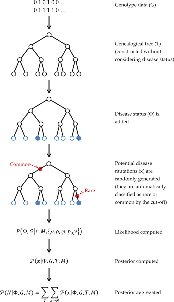
A flowchart (figure 2) illustrating the steps of our method is presented here. It is the diagrammatic representation of the algorithm in section 3.6. Here, we show that, at first, genealogical trees (actually, AR graphs) are generated from the SNP genotype (phased) data. Then, disease information is added for the subjects, and the disease likelihood is modeled, for which we simulate potential disease mutations at different branches of the tree. Using all these, the likelihood is computed, and then using appropriate priors, the posterior is calculated. The posterior is aggregated over simulated trees and mutations to give the final posterior distribution of rare and common variant counts.

Figure 2. Flowchart for the algorithm.

3.2 Bayesian Analysis

[Morris et al., 2002], [Zöllner and Pritchard, 2005] perform Bayesian analysis to obtain posterior probabilities of of the SNPs being (in LD with) the true DSLs. In the first step, they use the SNP genotype data (G) to generate possible ARGs (T) from the posterior P(T | G). In the next step, they evaluate posterior probabilities of the disease loci (x) given observed disease phenotypes (Φ) and the tree structure, i.e. P(x | Φ, T). The locus with the highest posterior probability can then be reported.

Our Bayesian analysis, while along the lines of [Zöllner and Pritchard, 2005], extends to complex diseases by allowing multiple DSLs with different penetrance. So, instead of a single DSL, we evaluate the posterior probability of a particular configuration of DSLs. Then, we evaluate posterior probabilities corresponding to counts of rare and common variants by aggregating over such posteriors.

Thus, instead of a single location, the vector x now contains all the information about (simulated) disease-susceptible mutations in the gene — the locations of the mutations, type of the mutation, as well as the allele at that locus. This x leads to a count of common and rare variants — denoted by the tuple N = (N_c, N_r). We can obtain P(N) by aggregating over P(x), and the posterior probability of the counts — P(N | Φ, T) is what we will be interested in.

3.3 The Likelihood

The likelihood has three terms in all — first, the probabilities of the minARGs given the SNP genotypes, P(T | G), secondly, the probabilities of the disease mutations occurring on a tree, P(x | T), and finally, the disease probabilities given the disease mutations, P(Φ | x, M). It will also include the modeling parameters, which we discuss later.

We will explicitly mention the disease model M, which includes models for the disease probabilities given the mutations, and involves models for penetrance, epistasis, phenocopy etc. In the initial stages of our calculations we keep the model M, as a conditional term, to clearly identify situations where those disease modeling assumptions play a role. We can later omit the term, as we consider it fixed.

3.3.1 Modeling the Tree

While modeling the tree, a simple top-down approach is taken. The root node has probability 1. Conditional on the parental node, a mutated offspring has probability μ, so a direct descendant, whose genotypes are same as his parent, has probability (1 − μ). Mutations are assumed to be independent. As each node only allows one mutation, if there are 𝒩 nodes in the tree, and m mutations, then the likelihood term for mutation is μ^m(1 − μ)^𝒩−m.

We also assume that mutation and recombinations are independent. If the probability of a recombination is ρ_j at locus j, at one particular node, the contribution is ${\rho }_j^r{(1-{\rho }_j)}^{1-r}$, where r indicates if there is a recombination or not.

3.3.2 Modeling the Mutations

Our model extends the approach of [Zöllner and Pritchard, 2005], where we had only one possible DSL, and since we do not know beforehand which SNP-interval it will belong to, it was assumed that without phenotype information the tree does not contain information about the DSL.

Now, since we have multiple mutations possible, one simple extension would be to model P(x | T,μ) = μ^k, where k is the total number of mutations in the tree that contribute to the disease. We still preserve the basic assumption that the tree topology by itself does not provide any information on the causal DSLs; this will be explained in detail in the discussion on priors (section 3.4).

3.3.3 Modeling the Disease Probability

As we have seen, the disease loci variable x contains the locations of the mutations, its type — rare/common, and the zygosity — 0/1/2 if common, 0/1 if it is a rare variant (as a person having two copies of the same rare variant is extremely low, without high inbreeding). These disease mutations are distinct from the marker SNP mutations, which are only used in making the trees.

Given a tree, a variant can be determined to be rare or common based on the threshold — if we take MAF < 1% to be the definition of rare variants, then by looking at where the mutation occurs in a tree, we obtain the proportion of people who have that mutation, and simply compare it with 1%SS.

While modeling the rare variants, we consider the mathematically simplifying assumption that if a subject has inherited any of the hypothetical (simulated) rare causal mutations, that individual will be diseased, i.e. complete penetrance. With completely penetrant rare variants, having a second rare variant in addition to the first one does not change the likelihood — that is the mathematical simplification we aim for. This is partly motivated by the standard infinite-sites model [Balding et al., 2007]. Note that this is not same as assuming that a person can have only one rare variant.

On the other hand, a person can have multiple common variants, each with small to moderate effect. Let c be the number of common variants a person carries, adding over all loci in the two chromosomes. The penetrance is modeled as a function of the common variant count c — it is easy to see that this function should be a positive non-decreasing concave function. That is so because, it is desirable that the gain in penetrance while moving from 20 to 21 common variants should be rather small than while moving from 1 to 2 common variants; if we used an additive or multiplicative instead, the change would have remained same or even increased, something which is not desirable. It also means that we do not enforce the common variants to have constant effect sizes. A suitable model for the penetrance is thus the power law, where p = p₀ · c^ν, where p₀ ≥ 1 is a multiplying factor (does not have the ‘base rate’ interpretation), c ∈ (0, 1) is the standardized count, and ν ∈ [0, 1] is the shape parameter. In this expression, the common variant count c is transformed to be in (0, 1) by dividing with the total number of loci.

We also allow for phenocopy, i.e. an individual can be affected without having any causal variants. It is modeled as P(disease | no variants) = φ, which is a small but non-zero quantity.

These modeling assumptions constitute our disease model M, and the results will certainly vary to some extent if a different model is used. To note, M comes only in the P(Φ | x, M) term.

3.4 Priors

We have denoted likelihoods by P(·), and we denote priors by π(·). Following the standard practice, we take π(T) and π(x) to be uniform. As mentioned in section 3.3.2, having a uniform prior on the tree topology on absence of any specific information is reasonable, and then our prior on the number of recombinations or mutations compensate for structures which have more mutations or recombinations, because they are rare events in reality. Also, if we do not have specific information about increased or decreased mutation rate in a specific part of the candidate region, it would be reasonable to assume that mutation is equally likely in any particular locus. One important point to consider is that these are proper uniform priors. This is so because the spaces of T and x are finite, as the number of possible minARGs is finite, and also any tree being of finite size, the number of possible mutations is also finite.

Now we put priors on the parameters μ, ρ, φ, p₀, ν. We do not go on to use hyperpriors on the prior parameters, but instead choose them carefully, e.g. the mean recombination rate from HAPMAP.

• Mutation rate: π(μ) = beta(α_μ, β_μ),

• recombination: π(ρ) = beta(α_ρ, β_ρ).

• Phenocopy: π(φ) = beta(α_φ, β_φ).

• Penetrance: π(p₀) =gamma(α_p, β_p); $\pi (\nu )=\frac{\text{log}\delta }{\delta -1}·{\delta }^{\nu },\delta \in (0,\infty )$.

The mutation, recombination and phenocopy rates are probabilities, and so it is standard to use a beta prior for them, as beta distribution is generally a conjugate prior for probabilities. For our real data analysis, we could estimate the rates from HAPMAP data extracted about the same region, and compute the prior parameters. In general, the program uses standard values provided in the literature, but since the probabilities can vary across the genomic region and the phenocopy rate might vary based on various environmental factors, the program allows for updated parameter values to better suit the dataset at hand. In Bayesian methods, the priors have a larger effect when the sample size is small, and the effect of the prior ’washes away’ as the sample size tends to infinity. So, especially for smaller sample sizes, the user can choose to vary the prior parameters themselves to see to what extent the posterior distribution is affected.

The parameters p₀ and ν have prior distributions chosen in a way such that they provide conjugate priors for the distribution of common variant penetrance described in the previous section and achieve the intended ‘positive non-decreasing concave’ shape.

3.5 Posterior

Because the parameters here are setwise independent, i.e. the three likelihood terms have different parameters, we can simplify the likelihood as (steps in appendix A):

$$P(\mathrm{\Phi },G|x,M,\{\mu ,\rho ,\phi ,p_0,\nu \})=\sum _{T}P(\mathrm{\Phi }|x,M,\{\phi ,p_0,\nu \})·P(x|T,\{\mu \})·P(T|G,\{\rho \}),$$

which can be written concisely, by integrating out the parameters, as

$$P(\mathrm{\Phi },G|x,M)=\sum _{T}P(\mathrm{\Phi }|x,M)·P(x|T)·P(T|G).$$

As with likelihoods P(·) and priors π(·), we denote posteriors by 𝒫(·). We are interested in 𝒫(x | Φ, G, M).

By Bayes rule, (note that π(x) is an uniform prior):

$$𝒫(x|\mathrm{\Phi },G,M)\propto P(\mathrm{\Phi },G|x,M)·\pi (x)\propto P(\mathrm{\Phi },G|x,M).$$

Note that P(Φ, G | x, M) can be easily obtained from the likelihood after integrating out the model parameters. That step is much simplified by observing again that the parameters are setwise independent, and therefore the three terms in the likelihood can be integrated independently. (Actually, μ contributes to both tree and mutation terms. But by the construction of coalescent trees, each SNP locus can mutate exactly once, and therefore the term involving μ is same for all trees. So we take it out of the calculations. Hence, μ remains only in the mutation term.) The details are in appendix B.

Hence, we can write,

$$𝒫(x|\mathrm{\Phi },G,M)=\sum _{T}P(T|G)·P(x|T)·P(\mathrm{\Phi }|x,M).$$

In the final stage, we summarize the information on mutations to the count vector N = (N_c, N_r), which stores the number of common and rare variants present in the case-control sample. Since are actually interested in is N, not x, so we aggregate over x to get the posterior distribution of N.

$$𝒫(N|\mathrm{\Phi },G,M)=\sum _T\sum _{x\to N}P(T|G)·P(x|T)·P(\mathrm{\Phi }|x,M)=\sum _{T}P(T|G)\{\sum _{x\to N}P(x|T)·P(\mathrm{\Phi }|x,M)\}.$$

3.6 The Steps for Computation

After describing the model in the previous sections, we now outline the steps for computing the posterior 𝒫(N | Φ, G, M), which is to be used for making inferences. These steps are also illustrated on the flowchart (figure 2) in the beginning of this section.

1. We use SNP haplotype data (G) to generate possible minARGs (T).

2. Given a tree (T), we model the likelihood P(x | T) of the putative DSL configurations (x), which depends on the probability of mutation and recombination at each site.

3. Next, we model the disease probabilities, P(Φ | x, T, M), where Φ is the disease status, M is the disease model.

4. They are used to simulate configurations of mutations (x) at probable DSLs. Each configuration corresponds to a particular count of common and rare variants, N = (N_r, N_c).

5. So the terms in the likelihood are: P(Φ | x, T, M), P(x | T), P(T | G). The complete likelihood P(Φ, G | x, M) aggregates the previous terms by summing over all possible T’s.

   $$P(\mathrm{\Phi },G|x,M)={\sum }_{T}P(\mathrm{\Phi }|x,M)·P(x|T)·P(T|G).$$

6. We use appropriate priors, e.g. uniform prior on trees (T), prior on recombination rate obtained from HAPMAP, etc.

7. We evaluate posterior probabilities 𝒫(x | Φ, G, T, M) of such configurations (x), given the observed phenotypes (Φ), SNP data (G), and the tree (T).

8. Finally, we get posteriors 𝒫(N | Φ, G, M) for variant configurations (N), by aggregating over corresponding configurations, and over simulated trees.

   $$𝒫(N|\mathrm{\Phi },G,M)={\sum }_T{\sum }_{x\to N}𝒫(x|\mathrm{\Phi },G,T,M).$$

The trees are generated in step 1 by Wu’s algorithm of generating minARGs uniformly from a given haplotype data. The mutations in step 4 are generated randomly on the branches of a given tree. Both these simulations are used for Monte Carlo estimates of probabilities by averaging, and therefore our computed posterior depends on the accuracy of the drawn samples — the number of draws and how well they span the sample space. As the sample space is finite in both cases, ensuring these criteria are much more straight-forward.

4 Results

4.1 Real Data Analysis

Nonsyndromic cleft lip with or without cleft palate (NSCL/P) is a common congenital malformation that is caused by an interplay of multiple genetic and environmental factors [Mossey et al., 2009]. Our dataset comprises 96 NSCL/P cases and 96 controls of Central European ethnicity in whom the exonic and adjacent intronic regions of one candidate gene for NSCL/P has been sequenced. The gene was among the candidate regions in an independent GWA study [Mangold et al., 2010]. Moreover, this gene has functional importance, as it codes for a protein which is involved in bone development, and is therefore relevant for further analysis.

The genotypes were obtained as unphased, and the software PHASE [Stephens et al., 2001], [Stephens and Donnelly, 2003] was used to infer the haplotypes. Phasing probability estimates were high in general (i.e. posterior probability computed by the software for the phase calls were mostly 100%, and in occasional cases going down to 85%, but never below). There was a single missing SNP in a person, and it was imputed using PHASE. The recombination rates estimated [Li and Stephens, 2003], [Crawford et al., 2004] from the data by PHASE tally with those from the CEU population of HAPMAP (phase II) [The International HapMap Consortium, 2007], which comments favorably on our data quality.

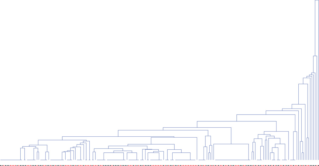
On a cursory comparison of the allele frequencies between cases and controls, it seems that lower-frequency SNPs have comparatively higher relative difference in terms of allele frequencies between the two groups, as compared to higher-frequency i.e. common variants. This implies that there should be some effect from rare variants. If we graphically display the generated ARGs for the data (a tree is shown in figure 3), they also imply that the top-level (i.e. higher MAF) SNPs do not provide a good partition of the cases and controls, whereas the lower-level SNPs provide small clusters of mostly cases and controls. These are scenarios where our algorithm, as expected, provide higher evidence for rare variants.

Figure 3. A simulated dendrogram for the dataset with cases and controls shown corresponding to the leaves, as red and black dots respectively.

Note that some subjects have identical genotypes and therefore are grouped together.

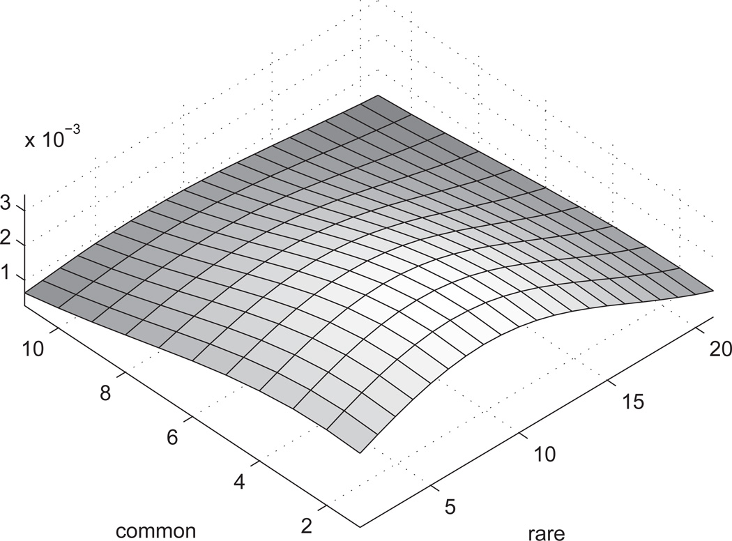
When we look at the obtained posterior distribution (figure 4) for the joint distribution of count of common and rare variants, we observe that the posterior mode is positioned along the axis of rare variants. The posterior dies out with increase in the number of common variants, which is expected to be the case when there are few or no common variants. Albeit, the posterior is not highly peaked, something to be expected given the small number of cases.

Figure 4. Smoothed posterior for real dataset.

The X and Y axes denote counts of rare and common variants, and the Z axis shows the (un-normalized) posterior density. The density is smoothed with a Gaussian kernel.

In fact, as the number of cases is only 96, the possible number of haplotypes is only 192, therefore for rare variants with MAF < 1%, on average we expect to see them in < 2 people. Such situations make it difficult to distinguish between real variant and phenocopy, therefore we can expect the detection efficiency to be low. But the posterior does indicate a skew towards rare variants, which is something we expect, based on our knowledge of the data. So we can conclude that the method works reasonably with this small sample too. In practice, as verified in our extensive simulations, for usual case-control studies with hundreds or even thousands of subjects, this method will have reasonably good performance.

Since we allow for phenocopy in our model, the posterior distribution also allows for the case with no causal variants in the genomic region, i.e. the (0,0) point. Thus, a posterior distribution comparing the presence or absence of causal variants in that region can also be derived from the current posterior distribution. That can lead to a statistical test for presence of causal variants, something which can complement the objective of this current paper, which works on a genomic region already identified as a potential candidate by a GWAS. It can be an interesting future project.

4.2 Simulated Data Analysis

We conduct a simulation study for a number of different scenarios - samples with no underlying variants, samples with only rare variants, with only common variants, and with both types of variants. Some (smoothed) plots of the bivariate posterior densities are produced as examples.

The haplotype distribution is generated by drawn the haplotypes from a coalescent genealogy via MaCS [Chen et al., 2009]. The loci are selected at random to be the DSLs with equal probability. The disease phenotypes are generated under various disease models (e.g. rare DSLs, common DSLs, both, or none), from which a specified number of cases and controls are selected without replacement. The causal loci are then excluded, following the assumption that the marker loci are not the DSLs. The number of SNPs is varied from 30 to 100, and similarly the number of causal rare and common variants. The sample size is also varied — we examine scenarios with total sample size ranging from 300 to 3000. Although we have taken equal number of cases and controls, it is not mandatory for our program. 1000 replications are typically used for calculating the posterior distribution, though this number can be changed easily.

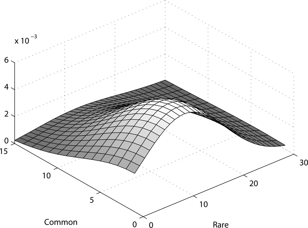
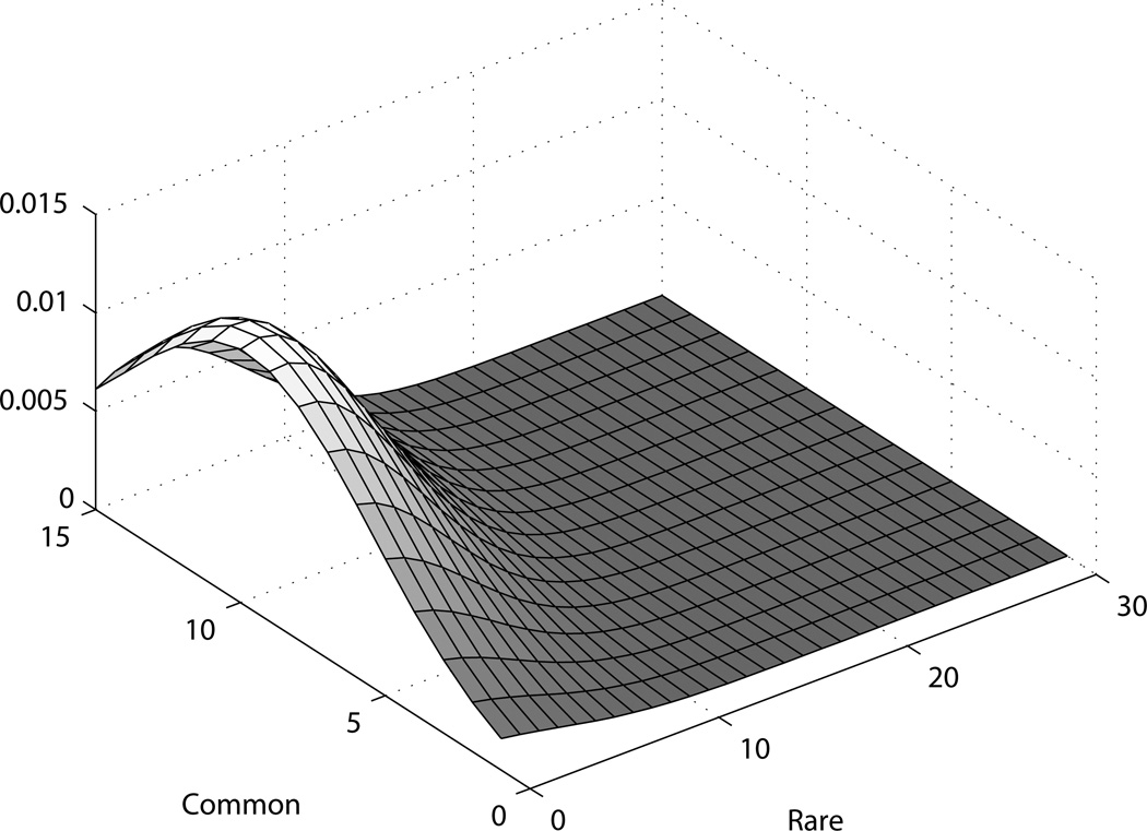
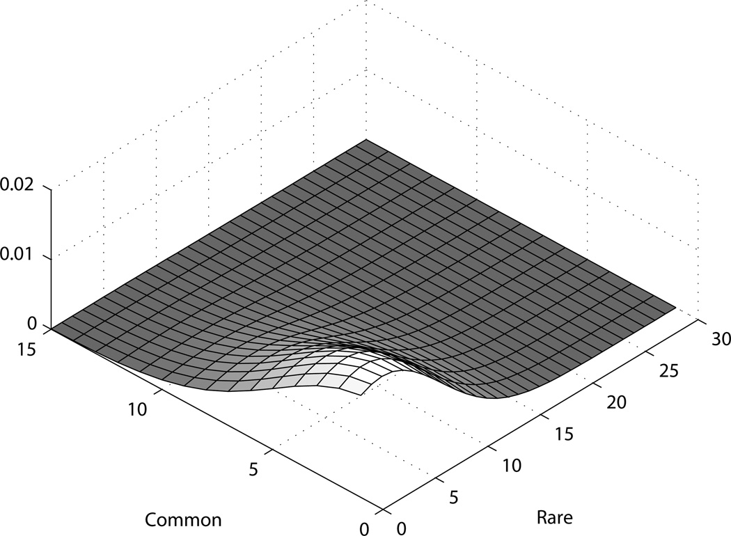
For all the figures presented here as examples, there is more spread in the posterior distribution on the axis of rare variants, as expected; both when there are true rare variants and when not. When there are true rare variants (figure 5), the posterior is shifted towards an increased count of rare variants. Similarly, for common variants as well (figure 6), the posterior is shifted more along the common variants axis as more common variants are added while simulating the dataset. For the scenarios presented here, we use 1000 cases and controls each, and 1000 replicates for the simulation. The data is generated as phase known.

Figure 5. Posterior for simulated dataset with rare variants.

Figure 6. Posterior for simulated dataset with common variants.

We observe that the peakedness of the posterior increases with the increase with sample size, which is natural, given that we get more information about the true number of variants. This is especially true for rare variants. As mentioned in the last section, when we have sample sizes of just a couple hundred, it is hard to distinguish rare variants from phenocopies. Then the posterior is largely dictated by the priors. But as we increase our sample size, given a true rare variant, we should see a cluster of affected people under some particular leaf of the genealogical tree. That is how we get increased efficiency to detect the presence of rare variants.

The posterior mode gives a rough idea about how many rare and common variants there are. This can be considered as an estimate, though is bound to have some variability, particularly in rare variants, as illustrated by the higher spread in that co-ordinate. We can see in figure 7, for example, that even under no true variant, the mode may be close to zero but not exactly zero.

Figure 7. Posterior for simulated dataset with no variants.

The simulated scenario with no true variants (figure 7) shows what can be considered of the null behavior for this method, where as the other cases reflect its efficiency. While that is somewhat model and parameter-dependent, it appears that the method does well in large samples; in the GWAS era, a sample of about a few thousand is not unexpected.

Although the tree sizes increases with the sample size, the tree nodes work with the haplotypes instead of the genotypes. And the number of possible haplotypes will be much less that the number of people, in particular if there is LD, which we expect to see in the small candidate regions that we work with. Thus, a moderate increase in sample size does not incur an unreasonable increase in tree computation.

5 Discussion

In this paper, we presented a method to predict the number of rare and common variants in a genomic region underlying a complex disease. While still based on SNP data, we are able to obtain information on this by utilizing the genealogical history inherent in the sample, by the use of genealogical trees (more specifically, ancestral recombination graphs). With a Bayesian approach, we provide a bivariate posterior distribution for the counts.

While being a Bayesian analysis, we avoid the use of Markov Chain Monte Carlo (MCMC) or Gibbs sampling to obtain posterior distributions, by taking simple conjugate likelihood and prior models. The choice of priors always has a scope of debate, and might be improved if more information is available from the studies of real datasets. For now, we try to incorporate as much available information as possible, e.g. using the mutation and recombination rates obtained from the HAPMAP. We think that this method can be extended by considering better models for rare variants, which can improve upon some simplifying assumptions.

By excluding such useful but computation-intensive methods, we are able to cut down on runtime, and the program runs under a few minutes for moderate sized datasets, even on personal computers. To be specific, with a few hundreds of subjects, and SNP counts around 30 to 100, the program runs in less that a couple minutes on a laptop (2.5GHz, 3 GB RAM), when we perform 500 simulations for each scenario. The program has fast computation speed for two reasons — first, we mostly use conjugate priors and are able to integrate mathematically, so we avoid Monte Carlo integrations for many variables (and we avoid MCMC altogether) — the computation time is mostly spent on simulating the trees and doing Monte Carlo integration. Secondly, the total number of unique haplotypes after phasing is much smaller than 2 × the total number of subjects, so the number of tree nodes in the ARG is much smaller than the expected number of nodes in a standard genealogical tree. However, as the computation required for trees increases rapidly with large number of SNPs, this method might not be well-suited for large datasets, e.g. a whole-genome scan, at this point; as the capability of computing infrastructure is increasing rapidly, and sequencing costs are also going down very fast, such extensions could become possible in the near future.

Another interesting way of extending this method would be to include covariates. Using covariates in order to better model the environmental effects, in addition to the genetic effects modeling, is becoming increasingly popular, and we could easily extend our method to allow for environmental factors by incorporating covariates into the phenocopy rate parameter.

At this point, we follow the standard assumption ([Wu, 2008], [Zöllner and Pritchard, 2005]) that that haplotype phase is known or readily available. But this method can be readily extended to include haplotype uncertainty. As the package PHASE provides haplotype estimates along with posterior probability estimates corresponding to those phase calls, those can easily be incorporated into our likelihood calculations, and simulations based on different phase configurations can be aggregated with phasing probabilities as weights, to produce the final posterior probability.

The method is fairly robust to population stratification, as it employs genealogical trees to model the population. It will be interesting to see how this method can be extended to family-based studies, which already contains some useful structural information, and is believed to be more powerful for studying rare variants.

Appendix

A. Simplifying the Likelihood

The parameters here are setwise independent, i.e. the the three likelihood terms have different parameters. We will later see why this is true. Then, we can simplify the likelihood as:

$$P(\mathrm{\Phi },G|x,M)=\sum _{T}P(\mathrm{\Phi },G|x,T,M)P(T|x,M)\approx \sum _{T}P(\mathrm{\Phi }|x,T,M)·P(G|x,T,M)·P(T|x,M)=\sum _{T}P(\mathrm{\Phi }|x,M)·P(G|T)·P(T|x)=\sum _{T}P(\mathrm{\Phi }|x,M)·P(x|T)·P(T|G).$$ [assumption A]

Assumption A says that given the complete ancestral history of both marker and disease loci, and given the disease model, the marker SNPs and disease phenotypes are independent. Which is reasonable given that the DSLs are not the markers, and we are conditioning on the DSLs directly. The next step follows as the model M only controls the disease probabilities.

Then we use that P(G | T) ∝ P(T | G)/P(T), and P(T | x) ∝ P(x | T) · P(T).

B. Simplification of the Likelihood Components

As mentioned in the deduction of posterior distributions, we integrate out the model parameters from the three likelihood components. This is facilitated by the parameters being setwise independent, which can be easily seen by looking at the three terms.

$$\begin{array}{c}\hfill P(T|G)=\int P(T|\rho ,G)\pi (\rho )d\rho ,\hfill \\ \hfill P(x|T)=\int P(x|\mu ,T)\pi (\mu )d\mu ,\hfill \\ \hfill P(\mathrm{\Phi }|x,M)=\int P(\mathrm{\Phi }|p_0,\nu ,\phi ,x,M)\pi (p_0)\pi (\nu )\pi (\phi )d{p}_{0}d\nu d\phi .\hfill \end{array}$$

C. A toy example

In the following simple example, we show how this method compares different tree structures based on their posterior (computed using likelihood and prior as disucessed below). we fix a tree and compute the posterior probabilities for different mutation configurations. Our data has 4 affected and 5 unaffected subjects. For simplicity, let

• p = P(disease|1 common variant) = 0.4,

• r = P(disease|rare variant) = 1,

• φ = P(disease|wildtype allele) = P(phenocopy) = 0.1,

• μ = P(mutation at any node) = 0.05.

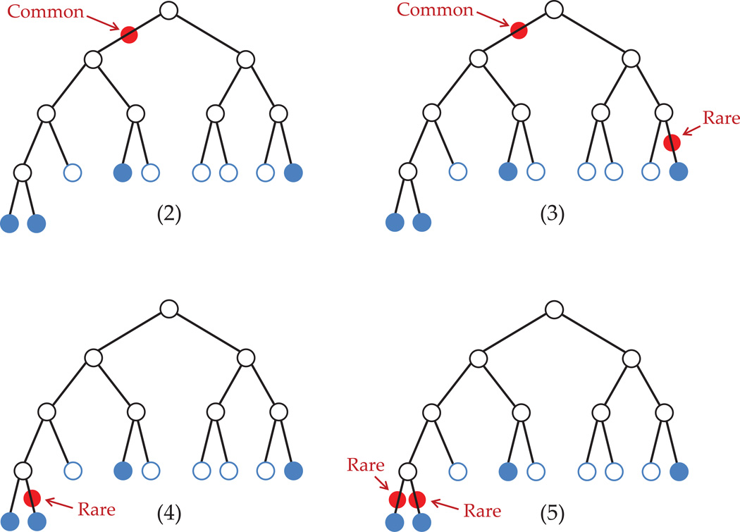
Given the tree structure, there are various possible configurations of DSLs. In figure 8, we show four such scenarios.

Figure 8. Some possible DSL configurations.

First, we compute P(Φ | x, T, M) = P(phenotype | mutations, tree, disease model).

1. If we had no mutations, i.e. only phenocopies;

   $$l=[{\phi }^4·{(1-\phi )}^5]=[{0.1}^4·{0.9}^5],\text{log}l=-9.7.$$
2. 1 common (MAF = 5/9), no rare variants;

   $$l=[p^3·{(1-p)}^2]\times [{\phi }^1·{(1-\phi )}^3]=[{0.4}^3·{0.6}^2]\times [{0.1}^1·{0.9}^3],\text{log}l=-6.4.$$
3. 1 common (MAF = 5/9), 1 rare variant (MAF = 1/9);

   $$l=[p^3·{(1-p)}^2]\times [r^1]\times [{(1-\phi )}^3]=[{0.4}^3·{0.6}^2]\times [1^1]\times [{0.9}^3],\text{log}l=-4.1.$$
4. 1 rare (MAF = 1/9), no common variants;

   $$l=[r^1]\times [{\phi }^3·{(1-\phi )}^5]=[1^1]\times [{0.1}^3·{0.9}^5],\text{log}l=-7.4.$$
5. 2 rare (MAF = 1/9), no common variants;

   $$l=[r^2]\times [{\phi }^2·{(1-\phi )}^5]=[1^2]\times [{0.1}^2·{0.9}^5],\text{log}l=-5.1.$$

Next, we compute P(x | T) = P(mutations|tree).

$$\text{log}l\propto \{\begin{array}{cc}\text{2 log}(1-\mu )=-0.1,\hfill & \text{no mutation}\hfill \\ \text{log}\mu +\text{log}(1-\mu )=-3,\hfill & \text{1 mutation}\hfill \\ 2\text{log}\mu =-6,\hfill & \text{2 mutations}.\hfill \end{array}$$

Combining these together, the total log-likelihood is:

$$\text{log}l=\{\begin{array}{cc}-9.8,\hfill & \text{no mutation}(1)\hfill \\ -9.4,\hfill & \text{1 common}(2)\hfill \\ -11.1,\hfill & \text{1 common},\text{1 rare}(3)\hfill \\ -10.4,\hfill & \text{1 rare}(4)\hfill \\ -11.1,\hfill & \text{2 rare}(5).\hfill \end{array}$$

Here, we have not evaluated all possible configurations (the ones with higher number of variants will have even smaller probability). Among those considered, case (2) with one common mutation seems most likely.

References

- Asimit J, Zeggini E. Rare variant association analysis methods for complex traits. Annual Review of Genetics. 2010;44(1):293–308. doi: 10.1146/annurev-genet-102209-163421. [DOI] [PubMed] [Google Scholar]
- Balding DJ, Bishop M, Cannings C. Handbook of Statistical Genetics. 3 edition. Wiley-Interscience; 2007. [Google Scholar]
- Bodmer W, Bonilla C. Common and rare variants in multifactorial susceptibility to common diseases. Nature Genetics. 2008;40(6):695–701. doi: 10.1038/ng.f.136. [DOI] [PMC free article] [PubMed] [Google Scholar]
- Chen GK, Marjoram P, Wall JD. Fast and flexible simulation of dna sequence data. Genome Research. 2009;19(1):136–142. doi: 10.1101/gr.083634.108. [DOI] [PMC free article] [PubMed] [Google Scholar]
- Crawford DC, Bhangale T, Li N, Hellenthal G, Rieder MJ, Nickerson DA, Stephens M. Evidence for substantial fine-scale variation in recombination rates across the human genome. Nature Genetics. 2004;36(7):700–706. doi: 10.1038/ng1376. [DOI] [PubMed] [Google Scholar]
- Dickson SP, Wang K, Krantz I, Hakonarson H, Goldstein DB. Rare variants create synthetic genome-wide associations. PLoS Biology. 2010;8(1):e1000294. doi: 10.1371/journal.pbio.1000294. [DOI] [PMC free article] [PubMed] [Google Scholar]
- Griffiths RC, Marjoram P. Ancestral inference from samples of DNA sequences with recombination. Journal of Computational Biology: A Journal of Computational Molecular Cell Biology. 1996;3(4):479–502. doi: 10.1089/cmb.1996.3.479. [DOI] [PubMed] [Google Scholar]
- Gusfield D, Eddhu S, Langley C. Optimal, efficient reconstruction of phylogenetic networks with constrained recombination. Journal of Bioinformatics and Computational Biology. 2004;2(1):173–213. doi: 10.1142/s0219720004000521. [DOI] [PubMed] [Google Scholar]
- Li N, Stephens M. Modeling linkage disequilibrium and identifying recombination hotspots using Single-Nucleotide polymorphism data. Genetics. 2003;165(4):2213–2233. doi: 10.1093/genetics/165.4.2213. [DOI] [PMC free article] [PubMed] [Google Scholar]
- Mangold E, Ludwig KU, Birnbaum S, Baluardo C, Ferrian M, Herms S, Reutter H, de Assis NA, Chawa TA, Mattheisen M, Steffens M, Barth S, Kluck N, Paul A, Becker J, Lauster C, Schmidt G, Braumann B, Scheer M, Reich RH, Hemprich A, Potzsch S, Blaumeiser B, Moebus S, Krawczak M, Schreiber S, Meitinger T, Wichmann HE, Steegers-Theunissen RP, Kramer FJ, Cichon S, Propping P, Wienker TF, Knapp M, Rubini M, Mossey PA, Hoffmann P, Nothen MM. Genome-wide association study identifies two susceptibility loci for nonsyndromic cleft lip with or without cleft palate. Nature Genetics. 2010;42:24–26. doi: 10.1038/ng.506. [DOI] [PubMed] [Google Scholar]
- Morris AP, Whittaker JC, Balding DJ. Fine-scale mapping of disease loci via shattered coalescent modeling of genealogies. American Journal of Human Genetics. 2002;70(3):686–707. doi: 10.1086/339271. [DOI] [PMC free article] [PubMed] [Google Scholar]
- Mossey PA, Little J, Munger RG, Dixon MJ, Shaw WC. Cleft lip and palate. Lancet. 2009;374:1773–1785. doi: 10.1016/S0140-6736(09)60695-4. [DOI] [PubMed] [Google Scholar]
- Schork NJ, Murray SS, Frazer KA, Topol EJ. Common vs. rare allele hypotheses for complex diseases. Current Opinion in Genetics and Development. 2009;19(3):212–219. doi: 10.1016/j.gde.2009.04.010. !ce:title¿Genetics of disease!/ce:title¿. [DOI] [PMC free article] [PubMed] [Google Scholar]
- Stephens M, Donnelly P. A comparison of bayesian methods for haplotype reconstruction from population genotype data. American Journal of Human Genetics. 2003;73(5):1162–1169. doi: 10.1086/379378. [DOI] [PMC free article] [PubMed] [Google Scholar]
- Stephens M, Smith NJ, Donnelly P. A new statistical method for haplotype reconstruction from population data. American Journal of Human Genetics. 2001;68(4):978–989. doi: 10.1086/319501. [DOI] [PMC free article] [PubMed] [Google Scholar]
- The International HapMap Consortium. A second generation human haplotype map of over 3.1 million SNPs. Nature. 2007;449(7164):851–861. doi: 10.1038/nature06258. [DOI] [PMC free article] [PubMed] [Google Scholar]
- Wu Y. Association mapping of complex diseases with ancestral recombination graphs: models and efficient algorithms. Journal of Computational Biology: A Journal of Computational Molecular Cell Biology. 2008;15(7):667–684. doi: 10.1089/cmb.2007.0116. [DOI] [PubMed] [Google Scholar]
- Zöllner S, Pritchard JK. Coalescent-based association mapping and fine mapping of complex trait loci. Genetics. 2005;169(2):1071–1092. doi: 10.1534/genetics.104.031799. [DOI] [PMC free article] [PubMed] [Google Scholar]