Using the Wash U Epigenome Browser to examine genome-wide sequencing data

Abstract

This unit describes the Wash U Epigenome Browser, a next-generation genomic data visualization system. The Browser currently hosts ENCODE and Roadmap Epigenomics data for human and model organisms. The Browser displays many sequencing-based data sets across all or part of the genome, on specific gene sets or pathways, and in the context of their metadata. Investigators can order, filter, aggregate, classify and display data interactively based on given feature sets including metadata features, annotated biological pathways, and user-defined collections of genes or genomic coordinates. Further, statistical tests can be performed on selected data. Individual labs can upload their sequencing or array-based data as custom tracks and display them in the context of consortium data, allowing for direct comparisons. The Browser is an increasingly important and widely accessible tool for deriving biological insights from unprecedented amounts of high-quality genomic, epigenomic and expression data.

INTRODUCTION

Newer and higher throughput genomic technologies, including next-generation sequencing, have revolutionized genome sciences. They have also generated unprecedented amounts of data. ENCODE and the NIH Roadmap Epigenomics projects alone have generated several thousand sequencing-based, genome-wide measurements of transcription factor binding and epigenetic marks including DNA methylation and histone modifications among others, in many cell types and tissues, creating a resource and reference for the scientific community. Additionally, small groups of researchers are able to rapidly obtain huge volumes of genomic and epigenomic data. Comprehensive analysis requires an informatics platform to integrate, visualize, and compare very heterogeneous datasets in the context of the rich metadata that accompany them.

The Wash U Epigenome Browser (a.k.a Human Epigenome Browser at Washington University in St. Louis, http://epigenomegateway.wustl.edu) represents a novel web-based genome browser designed to meet these needs. The Browser supports integration, visualization, and analysis of large, sequencing-based datasets. Genome-associated quantitative measurements are displayed as genome heatmaps wherein color gradients reflect strength of signal. Metadata such as cell type, assay type, epigenetic mark and phenotype of a sample are distinguished in the metadata color map alongside the genome heatmap. Investigators can zoom and pan in an intuitive style to examine as many as hundreds of datasets at detail levels ranging from whole-genome down to individual nucleotides. Data tracks can be sorted, organized, dragged and dropped individually or in combination with their metadata. Investigators can also toggle between heatmap views and height-based ‘wiggle’ plots. Additionally, investigators can visualize data for selected genomic features such as promoters, any set of genes or genomic coordinates, or any user defined pathways that can be dynamically obtained from popular pathway resources (e.g. KEGG; see UNIT 1.12). Investigators can also apply standard statistical analyses and display the results graphically on the browser. These features help investigators quickly obtain insights from genome-scale data that can be used to test, or even generate, hypotheses.

The Epigenome Browser currently hosts close to four thousand datasets from more than one hundred human cell/tissue types from the Human Epigenome Atlas and ENCODE projects. This includes an increasing number of full, single-base resolution DNA methylomes, profiles of different types of histone marks, locations of open chromatin, small RNAs, and strand-specific RNA-seq based expression and splicing profiles. The Browser is freely accessible to the public, and is being expanded to support model organisms including mouse and fruit fly. The Browser uses advanced, multi-resolution data formats that require minimal system resources and support remote data access. Thus, investigators can display their own genome-wide data and metadata on the Browser as custom tracks for direct comparison with reference data without having to transfer the entire dataset to the Browser. The Browser can be easily expanded to support any sequencing-based large genomics projects including many that focus on human diseases. The Epigenome Browse is an increasingly important and widely accessible tool for mining biological insights from unprecedented amounts of high-quality genomic, epigenomic and expression data.

This Unit walks reader through a series of examples to examine histone modification pattern over the human nicotinic receptor family genes. By following the instructions, reader shall be familiar with the Browser interface, be able to navigate around, bring up data sets of interest for display and interpret the data pattern. Reader will also be introduced to some advanced functions including genomic juxtaposition and Gene Set View, to focus the view on a subset of the genome; and the Gene Plot, to identify data pattern with respect to a gene set.

BASIC PROTOCOL. USING THE WASH U EPIGENOME BROWSER

The Wash U Epigenome Browser contains many components and offers diverse functionality. High accessibility is achieved through an advanced user interface. In this Protocol, major components and usability are illustrated by following a series of examples.

Necessary Resources

Hardware

Computer with Internet access, preferably with mouse-like pointing devices. On touch-screen devices, some peripheral features including cursor hovering effects will not work, but core functions won’t be affected.

Software

This web service runs best on open source web browsers including Chromium, Google Chrome, and Mozilla Firefox. Please upgrade your web browser to the most current version to achieve optimal performance. Microsoft Internet Explorer is currently not supported.

Display human gene CHRNA7 in the Browser

• 1In a web browser, open the Wash U Epigenome Browser home page at http://epigenomegateway.wustl.edu.

  1. On the Browser home page, click the first button on left to launch the Browser.

  2. Before the Wash U Epigenome Browser is fully loaded, a dialog box is displayed prompting the user to choose a genome assembly. To follow this Protocol, choose “Human hg19”. The Browser will continue to load and display default tracks belonging to the hg19 version of human reference genome.

  3. Survey the major Browser components (Fig. 1).

     The Browser panel is composed of the following major components. In the center is the genome heatmap, showing track data over a specific genomic position. Each row in the genome heatmap represents one track containing genome-wide numerical data. On the right side of the genome heatmap is the metadata color map, in which the metadata annotation of tracks in the genome heatmap are represented as different colors. Each column is one metadata term with the term name printed on top. Below the genome heatmap lie various genomic feature tracks aligned with the heatmap. The floating toolbox can be found on the top right of the Browser. It retains its position in the web browser window when the page is scrolled. The floating toolbox contains navigation buttons, the message console, and many other control options that remain hidden until invoked. At the bottom of the page is the control panel, whose left part is the navigation bar, and the actual interface is on the right. Clicking tabs in the navigation bar will reveal the corresponding control interface.

• 2Relocate to gene CHRNA7.

  1. In the floating toolbox, click the “Apps” button to show the list of applications. From this list, click the entry marked as “Relocation”. The “Relocate” panel will be displayed in the floating toolbox.

  2. Inside the “Relocate” panel, find the text field marked as “enter gene name”. Enter “CHRNA7” (input is case insensitive). Click the button “Jump” to relocate to this gene. In genome heatmap the displayed region has changed to gene CHRNA7.

• 3The gene CHRNA7 is on the forward strand of chromosome 15 (Fig. 2). By dragging the heatmap’s cursor to the right, the gene’s upstream region is exposed.
• 4Once at promoter region of CHRNA7, press the cursor on the chromosome band beneath the heatmap and drag it left or right to zoom into the selected region and reveal more details (Fig. 3).

Figure 1.

Annotated screen shot of the Browser panel. In this example the Browser is displaying default tracks from the human hg19 database, which consists of 36 sequencing experiment tracks in a genome heatmap, one gene track beneath the genome heatmap, and 6 metadata terms in a metadata color map. The genome heatmap is showing data in the default genomic location (chr10:20991666–25987500). These default settings can be changed by supplying parameters through the URL. Please refer to our online manual for information on how to customize the Browser display with URL parameters. Additionally, a short piece of text on top of genome heatmap provides information on the number of tracks on display in the genome heatmap, the genomic coordinates of the currently displayed region, and display resolution in the form of number of base pairs per pixel. Finally, users can press the cursor on the banner of the floating toolbox and move it around so it won’t block the view.

Figure 2.

Browser showing data over the CHRNA7 gene body. Gene models are visualized as “arrows on a line”. The arrows show the strand of the gene, in this case, the gene is on forward strand. Thus by scrolling to right, the gene’s upstream region on the left will be exposed. Coding exons are displayed as thick boxes, and un-translated regions (UTRs) as displayed as narrow boxes. Multiple gene models are present as the CHRNA7 gene has splice variants. Generally, the Browser displays the region covering longest gene model.

Figure 3.

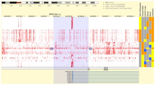
Zooming into the region containing CHRNA7 promoter. The transparent blue box is shown when cursor is pressed on the chromosome ideogram image and dragged. It marks the region to zoom into.

View histone modification data (H3K4me3) over the CHRNA7 promoter region

• 5The H3K4me3 histone mark (tri-methylation on lysine 4 of histone H3 protein) is a well-characterized histone modification type. It associates with open chromatin structures including some gene promoters. In this part of the protocol we will display many tracks from H3K4me3 ChIP-Seq experiments (chromatin immunoprecipitation and sequencing) and examine the status of this important histone mark over the CHRNA7 gene’s promoter.

  1. Go to the control panel at the bottom of the page and open the “Heatmap tracks” panel.

  2. The contents of “Track select panel” show the heatmap tracks available for display. Before proceeding, click the button labeled “remove everything” to remove all tracks displayed by default.

  3. By default, the heatmap tracks are organized by “sample types”, where their assay type attributes are not identified. Reconfigure the track selection panel using assay types.

     1. Click the button labeled “configure track selection panel” and a new box will be displayed. This box contains two drop-down menus that control how the track selection panel is to be organized.

     2. The menu on the left has the value “Sample”; change it to “Assay”.

     3. Click the button labeled “Generate track selection panel”. The track selection panel now has completely new contents. Close this box.

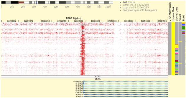
  4. Examine the contents in “Track selection panel”. A few high-level categories of assay types can be found including “Epigenetic Mark”, “Expression”, etc. If you click the label “Epigenetic Mark”, new labels with detailed contents are displayed at an indented level. Now sequentially click the “Histone Mark” label, “H3” label (stands for “histone H3 protein”), and finally the “H3K4” label (lysine 4 of H3). The label “H3K4me3” is now revealed as a non-clickable item (Fig. 4).

  5. Next to the label “H3K4me3” are a pair of numbers. The number in green indicates there are 141 total tracks that are H3K4me3 ChIP-Seq experiments. The other number indicates the number of tracks from this set currently on display. This number is red if the value is not zero. Select all the H3K4me3 tracks for display.

     1. Click the number pair to show a new panel in the floating toolbox. This panel contains all the 141 H3K4me3 ChIP-Seq tracks.

     2. Click the button labeled “All” to mark all tracks for submission.

     3. All tracks pending for submission are displayed in another panel in the floating toolbox. Click button labeled “Add these tracks” to submit them for display. It may take a moment before the data transfer completes. The wait time is determined by the number of tracks submitted and Internet connection speed.

  6. Once the data transfer completes, the height of the genome heatmap will increase substantially. Reduce the track height so that all tracks fit inside one screen.

     1. Right click on genome heatmap and select the “Configure” option. The track rendering options will now be displayed in the floating toolbox.

     2. Among the configuration options, check the box at bottom labeled “apply to all tracks”. This will make any subsequent change apply to all tracks in the heatmap.

     3. Change the track height to 2 pixels with the drop-down menu. This will set the height of all tracks to 2 pixels and convert the heatmap into a condensed view (Fig. 5).

• 6Examine the data pattern in the Browser (Fig. 5).

  It can be clearly seen that there is a strong H3K4me3 signal over the 3 kb region centered on the CHRNA7 transcription start site in most of the tracks, indicating the H3K4me3 mark is clearly present at CHRNA7’s promoter region in these samples. This suggests that the CHRNA7 promoter is in an open chromatin state and can be actively expressed. Focus the view on the group of tracks annotated by the metadata term “Blood”. If the tracks marked “Blood” are scattered among other tracks in the genome heatmap, group them together by clicking the word “Blood” on top of the metadata color map. In blood samples, the promoter H3K4me3 signal is not uniform among the various blood-cell types. Only in “mobilized CD34 primary cells” is strong H3K4me3 signal clearly observed. Otherwise no enrichment is observed and only background level signal is present in this region. Such absence of H3K4me3 enrichment can also be observed in other tissue samples including bone marrow and liver. This indicates the H3K4me3 pattern at the CHRNA7 promoter is regulated in a tissue-specific manner, and the CHRNA7 gene activity in these samples could be regulated in the same manner as well. However, to properly support such a hypothesis, data on other epigenetic marks and gene expression is needed.

Figure 4.

In the heatmap track selection function, heatmap tracks are organized as indented text trees for selection. The text tree is composed of metadata vocabulary terms and each line is one term. Terms on top of the tree can be clicked to reveal children terms. Click again to fold. Leaf level terms are not clickable. Other contents of the metadata vocabulary can be used to organize the track selection panel, and even two categories of metadata terms can be used to make a two dimensional grid. For this purpose go to the configuration options in the track selection panel and select a category using the second drop down menu. Most commonly the “Sample” and “Assay” are used in combination to generate such a track selection table.

Figure 5.

Genome browser showing H3K4me3 ChIP-Seq data over the promoter region of the human gene CHRNA7. The tracks in genome heatmap are from the Roadmap Epigenomics Project and contain read density count of the sequencing experiments. These tracks are rendered in red with automatic scale, which is the default setting and can be customized by selecting the “Configure” option in the right-click menu. Heatmap cells with the most intensive red color indicates read density values close to the maximum read density value over the entire genomic region in the genome heatmap. Experimental samples belonging to categories of “ES/iPS Cells”, “Breast”, and “Blood” are indicated in respective columns in the metadata color map. Users can go to the metadata configuration panel and add more metadata categories to reveal extra attributes of the tracks in the genome heatmap. A gene track is displayed beneath the genome heatmap showing part of the CHRNA7 gene. Multiple gene models are tiled vertically and they are alternatively spliced variants of the same gene. Clicking on any one of the genes, a tooltip will be displayed showing brief information about that gene.

Juxtapose data to focus on a subset of the genome

• 7Run data juxtaposition on gene bodies.

  1. Find the gene track below the genome heatmap. Right click on the track image to get the context menu. Select the “Juxtaposition” option from the menu. The Browser is now juxtaposing data by items in the gene track.

  2. Examine the Browser view (Fig. 6).

     By running juxtaposition, the Browser is showing the data over genes in the gene track, but not data over the intergenic regions. Click the “zoom out” button in the floating toolbox to include more genes in the view. Scroll the genome heatmap to expose nearby genes. This view provides a quick survey of H3K4me3 patterns over CHRNA7 and its neighbors. Notice gene KLF13 to the left. It has a strong H3K4me3 signal at its 5′ end in almost all samples, and shows strong gene body H3K4me3 signals in some blood samples. Refer to the right and find GREM1, this gene also has strong H3K4me3 signals at the gene’s 3′ end in many samples, but lacks a 5′ end signal in blood samples, indicating GREM1 might not be active in blood and immune cells.

• 8Re-run the data juxtaposition on the gene promoters.

  1. If the Browser is still running juxtaposition, turn it off by right clicking on the gene track and select the “Undo juxtaposition” option. The Browser will return to genomic view.

  2. Display gene promoter track.

     1. At the control panel, click the “Tracks” tab, then the “Genomic features” tab. The genomic feature track management panel will be displayed on right.

     2. In the genomic feature control panel, click the button labeled “Add more” and a small panel appears prompting the user to select genomic feature tracks.

     3. This genomic feature selection panel has two parts: On the left side lists the groups. Click the group labeled “Genes” to highlight. Gene tracks will be displayed on the right side. Next to the gene track name is a downward pointing arrow. Click this arrow to reveal the promoter track associated with this gene track. Click on the promoter track name and it will be added to the list in the control panel.

     4. Move back to the genomic feature track management panel, and turn off the gene track and turn on the promoter track using the drop-down menus with each track. Each item in the promoter track is a 3 kb region upstream of the transcription start site of one gene.

  3. Right click on the promoter track and select the “Juxtaposition” option. The Browser is now juxtaposing data by items in the promoter track.

  4. Examine the Browser view (Fig. 7).

     The Browser is showing H3K4me3 data over the gene promoters. You can scroll or zoom to adjust the viewing region. Strong H3K4me3 signal presents at some gene promoters, including CHRNA7, KLF13, and FAN1. Conversely, many other promoters are lack H3K4me3 signal, indicating these genes might be inactive in these samples. Among the genes having strong H3K4me3 signal over their promoters, CHRNA7 stands out by showing a patchy pattern (H3K4me3 signal exists in a subset of the samples), while the KLF3 and FAN1 promoters show a consistently strong H3K4me3 signal over all samples.

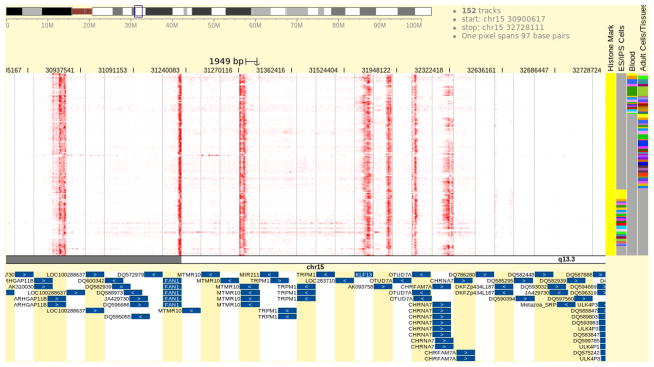
Figure 6.

Data is juxtaposed to reveal H3K4me3 patterns on CHRNA7 and its surrounding neighbors. To contrast with neighboring genes, a grey line is drawn vertically between genes in the genome heatmap, and alternating background colors (white and yellow) are used for neighboring genes in the gene track. In the gene track, it is seen that OTUD7A and CHRNA7 have different background colors, indicating the non-genic region between them is not shown. But CHRNA7 is sharing the same background color with DKFZp434L187 and some other genes because these genes overlap, sharing the same segment in the view.

Figure 7.

The Browser is juxtaposing data to reveal H3K4me3 patterns on promoter regions with CHRNA7 and its neighbors. The display style is the same as explained in Figure 4.

View H3K4me3 patterns over the nAChR (nicotinic receptor) gene family using the Gene Set View

• 9Quit data juxtaposition if the Browser is in juxtaposition mode. Right click on any genomic feature track and select “Undo juxtaposition” option to quit.
• 10At the control panel click the “Genomic view” tab, then the “Gene Set View” tab. The “Gene Set View” control panel will be displayed on right.
• 11Enter gene names in the text area and run Gene Set View.

  1. Click the “Clear” button to remove the default gene list from the text area.

  2. Enter names of the nAChR family of genes into the text area: “CHRNA1”, “CHRNA2”, “CHRNA4”, “CHRNA7”, “CHRNA9”, “CHRNA10”, “CHRNB1”, “CHRNB2”, “CHRNE”, “CHRNA5”, “CHRNA3”, “CHRNB4”, “CHRNB3”, “CHRNA6”, “CHRND”, “CHRNG”. Names must be separated by line breaks.

  3. Press the “Submit” button to run Gene Set View using these genes.

  4. Examine the Browser view (Fig. 8).

     The H3K4me3 signal appears strongly in a subset of the nAChR gene family (CHRNA7, CHRNB1, CHRNE, CHRNA5). Most of the signal appears at 5′ end of the genes, which is consistent with the previous observation of H3K4me3 pattern on the CHRNA7 gene’s promoter. Quite extraordinary is the CHRNB1 gene, where the H3K4me3 signal is observed in the highest intensity over the second to last exon of this gene (zoom in and enlarge this gene to get a detailed view). The H3K4me3 mark also shows a spreading pattern over the CHRNE gene body.

• 12Re-make the Gene Set View using 5 kb regions centered over transcription start sites of the genes.

  1. Go to the Gene Set View control panel and find a new panel above the submission interface. This panel contains editing options to apply to the existing gene set. At its top banner click the “Change part” tab. New contents will be displayed in this panel.

  2. By default, genes are displayed with their gene bodies (the genomic interval starting from transcription start site to stop site). To change, click the button labeled “change”. A panel appears with options. Choose the option “custom region...” and further contents are displayed in this same panel.

  3. Drag the green slider to the left and select 2500 bp. Drag the red slider to the right and select 2500 bp. Check the option “transcription start site”. This will select the 5 kb region centering over transcription start site as a “custom region”.

  4. Click button “Update” to take effect.

  5. Examine the Browser view (Fig. 9).

     Similar to the gene body view in Fig. 6, a strong H3K4me3 signal is found in a subset of nAChR family genes at the regions around the transcription start sites. As demonstrated in Fig. 3, the region belonging to CHRNA7 shows a patchy pattern where the H3K4me3 signal is observed in a subset of samples. A strong consistent H3K4me3 signal can be found in the CHRNA5 region.

Figure 8.

Gene Set View of the H3K4me3 signal over the nAChR family genes. In this view, genes are tiled to form the horizontal axis of the genome heatmap. A gray line is plotted between every two genes in the genome heatmap. Under the genome heatmap, the chromosome bar is replaced by a graph of hollow boxes, which serve as a visual indication of the genes. The user can drag this bar to zoom in and get a detailed view over regions of interest, and drag the genome heatmap to scroll. The content of the gene track at the bottom updates accordingly. Genes have been arranged by their order of submission, but can be rearranged or sorted using editing options in the control panel.

Figure 9.

Gene Set View of the H3K4me3 signal over the 16 genes in the nAChR family. Unlike Fig. 6, the 5 kb regions centering over the transcription start sites are displayed for every gene. As a result, 16 equal length regions are present in this view. In in the gene track at the bottom, only partial gene structures are shown instead of complete genes. Beneath the genome heatmap where the chromosome bar used to be, filled rectangles are drawn to indicate each region. The green half of rectangle indicates the portion of the upstream region relative to the gene’s transcription start site, and likewise the red-filled half indicates the downstream part of the region. Orientation of the red/green filling is determined by the gene’s strand. The user can still drag on this graph to zoom in and see detailed data patterns and scroll to explore.

Run Gene Plot over the genes

• 13Scroll down the page and go to the Gene Set View control panel (click “Genomic view” tab, then “Gene Set View” tab to show this panel). Find the button labeled “Gene Plot” and click it to show the Gene Plot panel hovering above the web page. This runs Gene Plot with the set of genomic intervals being used for Gene Set View following Step 12 of this Protocol.
• 14At the “Step 1” section of the Gene Plot panel, click the “select” button and select a track. Only tracks with numerical data can be selected. Data from this track will be used for Gene Plot. For demonstration purposes we select the “H3K4me3 of mobilized CD34 primary cells” track.
• 15At the “Step 2” section of the Gene Plot panel, choose the “hierarchical clustering” for graph type. The configuration options associated with hierarchical clustering will be displayed on the right. Select “euclidean” for a distance metric. Set “Row height” and “plot width of data points” to their maximum values to enlarge the graph to be generated as we only have 16 genomic intervals to plot with (from Step 12 of the Protocol). If many genes are to be handled, use smaller values for “Row height”.
• 16Skip “Step 3”. At the bottom of the panel click the “Make gene plot” button. The plot will be made and displayed in the same panel.
• 17Examine the plot (Fig. 10).

  This plot shows a clustering pattern of genomic intervals with respect to the H3K4me3 ChIP-Seq track. In the plot a heatmap visualizes data from the particular H3K4me3 track over the genomic intervals, so that the data pattern at different intervals can be contrasted and the variance can be brought out. Each line in the heatmap belongs to one genomic interval. The maximum data value over all genomic intervals is used to set the color of the heatmap cells, so dark red indicates a data value close to the maximum. On the left of the heatmap a dendrogram shows how genomic intervals are grouped together by hierarchical clustering. Genomic intervals belonging to genes CHRNA5 and CHRNA7 are set apart from other intervals, as they harbor the strongest H3K4me3 signal. Because the peaks of the signals occur at different locations, the two genes do not belong to the same sub-cluster.

Figure 10.

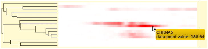
Hierarchical clustering of genes reveals how H3K4me3 marks are distributed across the genomic intervals belonging to the nAChR gene family. Move the cursor over the heatmap to view the gene name and data value of the heatmap cell under the cursor. In the heatmap, genes from top to bottom are: CHRNA5, CHRNA7, CHRNB4, CHRNB1, CHRNE, CHRND, CHRNB2, CHRNA4, CHRNA6, CHRNG, CHRNB3, CHRNA1, CHRNA9, CHRNA10, CHRNA3, CHRNA2. To select genes inside a sub-cluster, click the splitting point of that sub-cluster in the dendrogram and the list of genes will be displayed in a table below the graph.

COMMENTARY

Background Information

The Wash U Epigenome Browser is a powerful web service for visualizing whole-genome data sets, especially high-throughput DNA sequencing data. It extends the UCSC Genome Browser (Dreszer et al., 2011, UNIT 1.4) and the UCSC Cancer Genomics Browser (Sanborn et al., 2011) and it features novel functions. It is rooted in the well-known and dependable UCSC Genome Browser code base, achieving optimum server performance, and it adopts the twin-heatmap visualization approach of the Cancer Genomics Browser in visualizing data. The Wash U Browser focuses on hosting public data sets. At the moment its data comes exclusively from large consortium projects where data are produced in massive amounts and scope of coverage, and are relatively easy to collect and assemble. As of May 2012, the Wash U Browser is hosting over 4000 sequencing experiment tracks from the Roadmap Epigenomics (http://www.roadmapepigenomics.org/) and ENCODE (http://genome.ucsc.edu/ENCODE/) Projects. With the Wash U Browser, it is possible to navigate such enormous and diverse datasets and mine for biological information. Investigators can have 500+ tracks of various types and sources displayed in a single screen, and group the tracks in a meaningful way by the metadata attributes so that data patterns can be revealed. Facet browsing ensures investigators are able to identify tracks of interest in a directed and progressive manner. The Wash U Browser is sophisticated inside, but with its intuitive user interface, simple tasks are made easy and complicated tasks are made possible.

Genome annotation data used by the Wash U Epigenome Browser are downloaded from the UCSC Genome Browser database. The data are presented in the form of various genomic feature tracks and are assigned into meaningful groups for easy identification. In helping investigators analyze and understand sequencing experimental data in the context of genomic annotations, various unique functionalities have been developed, including data juxtaposition, Gene Set View, and Gene Plot, as demonstrated in this Unit. These functionalities allow investigators to view data from diverse angles and obtain insights that are otherwise difficult to achieve with conventional genome browser displays.

Engineering-wise, the Wash U Browser adopts the latest web technologies to deliver the best user experience. All client-server interactions are through Ajax protocol, which updates website content without reloading the web page. The Browser processes much of the tasks on the user’s web browser, including facet browsing and track rendering, thus reducing server queries to the minimum amount. Tracks can be re-rendered with custom styles at the blink of an eye. All these features contribute to a thoroughly modern web tool with satisfying performance and response.

The protocols in this Unit cover the essence of the Wash U Browser, including relocating to a genomic location, selecting tracks via the facet browsing function, scrolling and zooming to adjust the view, and data juxtaposition and Gene Set View to focus on a specific features of the genome. While these contents should adequately address most of the expectations about what a genome browser should accomplish, the Wash U Browser is nonetheless equipped with an array of advanced features that are not demonstrated here due to requirements of extra specialty and resource. These features apply special visualization techniques or automate routine tasks, and can be tremendously useful in specific contexts. Following is brief description about them.

Statistical analysis functions

Functions in this category include correlation analysis, pairwise comparisons, and hypotheses testing. With them the user can perform preliminary and explorative analyses on the data displayed in the genome heatmap. The correlation function assesses similarity between a target track and other tracks in genome heatmap. Track data from the current view in the genome heatmap is used for the correlation, but data beyond the view is not. To compare two groups of heatmap tracks, pairwise comparisons can be used to calculate the log2(ratio) as a straight-forward metric. These values are rendered as a quantitative track below the genome heatmap to show the comparison’s result. For rigorous comparisons, hypotheses tests can be used to derive P values as a measure of track data variation. Similar to the log2(ratio) track from the pairwise comparisons, a track of P values will be displayed to visualize the hypothesis test result. A P value cutoff can be set to select genomic intervals showing significant P values from the test.

Bird’s eye view

This function helps user obtain the “whole picture” on any track from the Browser. The user can select a genome heatmap track and view its data pattern over all chromosomes via the bird’s eye view. Gene tracks can also be displayed in same way, but gene density data will be displayed instead. The bird’s eye view function is versatile enough to display multiple tracks in the same view so that they can be contrasted and customized with different colors and scales. Even log2(ratio) or P value data from statistical analyses can be displayed showing genome-wide comparison results.

Custom track and dataHUB

The custom track function helps the user display their private data; this is very useful as the custom tracks behave in the same way as native tracks. Users can visualize their custom track alongside the native tracks, and apply all analysis and visualization techniques, for example running juxtaposition with a custom genomic feature track. Data must be prepared into binary, indexed file formats (bigWig, or bigBed as described in Kent WJ, 2010, and BAM as described in Li H, 2009), and the files will be placed on a web server for access. Such network-based file access is fast and secure, as only the small portion of data used for display is read and transmitted and never requires any file upload. Fortunately, the preparation procedures of custom track files are standardized and require only modest hardware investment and routine bioinformatics skills.

The dataHUB function is a natural extension of the custom track function. With dataHUB, the user can organize all of his/her custom tracks in one place, and display them on the Browser with one single step instead of laborious one-by-one uploading. Tracks inside a hub can be a mixture of types (quantitative data, annotation data, read alignment) and are not restricted to be on the same web server or host. Moreover, users can define custom metadata and annotate tracks to intelligently identify and organize everything in the hub. The dataHUB function doesn’t restrict the number of tracks in a hub and is a light-weight, yet powerful tool for building centralized collections of genomics data on the web.

URL parameters and the session function

These functions create a record of the user’s browsing status. Via the URL parameters, the user can control the contents displayed in the Browser, such as genome assembly, set of tracks, and genomic position on which to show the data. Users can compose such a URL and share their customized contents. Alternatively, session functions can be used to record a user’s browsing status. This saves a user’s status in a database on the server that can be retrieved by a session ID. Saved session information can be kept in the database for a limited time period, usually 3–6 months, and the URL parameter has virtually unlimited life span and is a preferred way of making one’s browsing status permanent.

Conclusion

The Wash U Epigenome Browser is always under active development in order to adapt to the fast-paced field of genome science. New feature releases, bug fixes, and adjustments to existing features happen regularly. Users can always refer to our online manuals for up-to-date instructions at http://epigenomegateway.wustl.edu/browser/manual/, and are recommended to subscribe to our blog (washugb.blogspot.com) or twitter feed (@WashUGBrowser) to receive news and announcements.

Literature Cited

- Dreszer TR, Karolchik D, Zweig AS, Hinrichs AS, Raney BJ, Kuhn RM, Meyer LR, Wong M, Sloan CA, Rosenbloom KR, Roe G, Rhead B, Pohl A, Malladi VS, Li CH, Learned K, Kirkup V, Hsu F, Harte RA, Guruvadoo L, Goldman M, Giardine BM, Fujita PA, Diekhans M, Cline MS, Clawson H, Barber GP, Haussler D, Kent WJ. The UCSC Genome Browser database: extensions and updates 2011. Nucleic Acids Res. 2012;40(Database issue):D918–23. doi: 10.1093/nar/gkr1055. [DOI] [PMC free article] [PubMed] [Google Scholar]
- Sanborn JZ, Benz SC, Craft B, Szeto C, Kober KM, Meyer L, Vaske CJ, Goldman M, Smith KE, Kuhn RM, Karolchik D, Kent WJ, Stuart JM, Haussler D, Zhu J. The UCSC Cancer Genomics Browser database: update 2011. Nucleic Acids Res. 2011;39(Database issue):D951–9. doi: 10.1093/nar/gkq1113. Epub 2010 Nov 8. [DOI] [PMC free article] [PubMed] [Google Scholar]
- Kent WJ, Zweig AS, Barber G, Hinrichs AS, Karolchik D. BigWig and BigBed: enabling browsing of large distributed datasets. 2010;26(17):2204–2207. doi: 10.1093/bioinformatics/btq351. [DOI] [PMC free article] [PubMed] [Google Scholar]
- Li H, Handsaker B, Wysoker A, Fennell T, Ruan J, Homer N, Marth G, Abecasis G, Durbin R. Genome Project Data Processing Subgroup, 2009. The Sequence alignment/map (SAM) format and SAMtools. Bioinformatics. 1000;25:2078–9. doi: 10.1093/bioinformatics/btp352. [DOI] [PMC free article] [PubMed] [Google Scholar]
Key Reference
- Zhou X, Maricque B, Xie M, Li D, Sundaram V, Martin EA, Koebbe BC, Nielsen C, Hirst M, Farnham P, Kuhn RM, Zhu J, Smirnov I, Kent WJ, Haussler D, Madden PAF, Costello JF, Wang T. The Human Epigenome Browser at Washington University. Nature Meth. 2011;8:989–990. doi: 10.1038/nmeth.1772. The original publication describing Wash U Epigenome Browser’s innovative designs and critical applications. [DOI] [PMC free article] [PubMed] [Google Scholar]