Genome-wide Association Analysis for Multiple Continuous Secondary Phenotypes

Abstract

There is increasing interest in the joint analysis of multiple phenotypes in genome-wide association studies (GWASs), especially for the analysis of multiple secondary phenotypes in case-control studies and in detecting pleiotropic effects. Multiple phenotypes often measure the same underlying trait. By taking advantage of similarity across phenotypes, one could potentially gain statistical power in association analysis. Because continuous phenotypes are likely to be measured on different scales, we propose a scaled marginal model for testing and estimating the common effect of single-nucleotide polymorphism (SNP) on multiple secondary phenotypes in case-control studies. This approach improves power in comparison to individual phenotype analysis and traditional multivariate analysis when phenotypes are positively correlated and measure an underlying trait in the same direction (after transformation) by borrowing strength across outcomes with a one degree of freedom (1-DF) test and jointly estimating outcome-specific scales along with the SNP and covariate effects. To account for case-control ascertainment bias for the analysis of multiple secondary phenotypes, we propose weighted estimating equations for fitting scaled marginal models. This weighted estimating equation approach is robust to departures from normality of continuous multiple phenotypes and the misspecification of within-individual correlation among multiple phenotypes. Statistical power improves when the within-individual correlation is correctly specified. We perform simulation studies to show the proposed 1-DF common effect test outperforms several alternative methods. We apply the proposed method to investigate SNP associations with smoking behavior measured with multiple secondary smoking phenotypes in a lung cancer case-control GWAS and identify several SNPs of biological interest.

Introduction

Genome-wide association studies (GWASs) have become a popular approach for identifying common genetic variants that are associated with disease phenotypes and quantitative traits. Hundreds of GWASs have been conducted in the last few years and have identified over 1,000 disease- and trait-associated common single-nucleotide polymorphisms (SNPs).¹ Many existing GWASs use a case-control design, in which hundreds of thousands of SNPs are genotyped in a large number of disease-affected and disease-free individuals in order to identify SNPs that are susceptible to diseases.^2,3,4 There is substantial interest in leveraging these existing large case-control GWASs in order to identify common variants associated with multiple secondary phenotypes that are often collected in these case-control GWASs. For example, in the lung cancer (MIM 211980) GWAS conducted at Massachusetts General Hospital (MGH), four continuous traits measuring smoking behavior were collected for both affected and control individuals, including the age of smoking initiation, smoking duration, average number of cigarettes per day (CPD), and number of years of smoking cessation. It is of interest to conduct a GWAS analysis for the identification of SNPs that are associated with smoking behavior by jointly analyzing four smoking phenotypes while accounting for case-control ascertainment bias.

Numerous GWAS analyses have been performed for continuous traits, such as body mass index,⁵ age at menarche,⁶ and height.⁷ A standard approach for GWAS analysis of continuous traits in cross-sectional and cohort studies is to fit a linear regression model for each trait separately. Because of the large number of SNPs analyzed, GWAS analysis is plagued with a substantial multiple-testing burden, making it challenging for SNPs to reach genome-wide significance levels (e.g., p values $<{10}^{-7}$). Furthermore, given that common variants often have weak effects, as observed in many GWASs of complex traits,¹ many top SNPs identified in a GWAS are false positives.

Consequently, it is of substantial interest to develop testing strategies to improve power in identifying SNPs with weak effects in GWASs. Because multiple secondary traits are likely to be correlated and to measure the same underlying trait in different dimensions, joint analysis of these traits by taking into account their correlation is likely to improve power in comparison to individual trait analysis. In particular, joint analysis of multiple phenotypes can borrow information across correlated multiple phenotypes and increase effective sample sizes.⁸ Such joint phenotype analysis also allows for the study of pleiotropic effects.

However, when analyzing secondary phenotypes with case-control designs, one needs to be mindful of ascertainment bias. As described in Monsees et al.,⁹ in the context of a single secondary phenotype, the bias is generally small for analyses that ignore ascertainment or stratify on case-control status, provided the marker is independent of disease risk. Additional care must be taken when there is evidence that both the secondary trait and the tested genetic marker are associated with the primary disease. For example, in the smoking GWAS analysis conducted in this paper with lung cancer case-control samples, it is likely that the same SNPs might be associated with both smoking and lung cancer.^10,11 In this situation, naive analysis ignoring case-control sampling is likely to result in bias in the association analysis of smoking behavior. Monsees et al.⁹ showed that inverse probability weighted (IPW) regression for a single continuous outcome provides unbiased estimates of marker-secondary trait association. Lin and Zeng¹² developed a retrospective likelihood method for analyzing a single secondary phenotype in case-control association studies. However, to date, the joint analysis of multiple secondary phenotypes in case-control designs has not been explored.

For cross-sectional and cohort studies, multivariate regression methods, such as multivariate ANOVA¹³ and generalized estimating equations,⁸ provide valuable tools for analyzing multiple-phenotype data. These models often use multiple degree of freedom (M-DF) tests to assess the effects of an independent variable on multiple phenotypes while accounting for the correlation between phenotypes within the same individual. When multiple phenotypes measure the same underlying trait in the same direction (after transformation), power can be improved by testing the shared or common effect of an independent variable on multiple phenotypes. Specifically, in view of the fact that positively correlated continuous phenotypes are often measured on different scales, Roy et al.¹⁴ proposed a scaled marginal model for testing and estimating the shared common effect of an independent variable on multiple phenotypes in cross-sectional and cohort studies, where a one degree of freedom (1-DF) test was developed on the basis of estimating equations.

In this paper, we extend the work of Roy et al.¹⁴ and propose a scaled marginal model for genome-wide association analysis of multiple continuous secondary phenotypes in case-control studies. Specifically, when multiple phenotypes are positively correlated and measure the same underlying trait in the same direction (after transformation), we propose the use of IPW-estimating equations in order to estimate and test the shared common effect of SNPs on multiple continuous secondary phenotypes in case-control studies. This approach accounts for case-control ascertainment in analysis of secondary phenotypes with the use of disease-prevalence-based inverse probability weights. We term the proposed test the scaled multiple-phenotype association test (SMAT). By jointly estimating outcome-specific scale parameters with scaled marginal models, the proposed SMAT method tests for the common effect of SNP with a 1-DF test while allowing for phenotype-specific covariate effects. As an estimating-equation-based approach, it accounts for arbitrary correlation among multiple phenotypes and is robust to departure from normality and misspecification of correlation among multiple continuous phenotypes. Furthermore, the assumption of common effect can be tested with an estimating-equation-based score test by comparing scaled marginal models with heterogeneous SNP effect models.

Our simulation studies show that, when multiple phenotypes (after transformation) are positively correlated and measure the same underlying trait or disease process in the same direction, and if the scaled effects of multiple phenotypes are homogeneous or moderately heterogeneous, the proposed 1-DF test SMAT for the common effect of SNPs on multiple correlated phenotypes is more powerful than either testing the outcomes separately or testing the outcomes jointly with the traditional M-DF test. In addition, type I error is preserved in the presence of not only case-control sampling but also heterogeneous SNP effects that depart from the scaled marginal model with common effect. We apply the proposed method to joint analysis of the four smoking phenotypes in the MGH lung cancer GWAS, which leads to the identification of several top SNPs of biological interest.

Material and Methods

The goal of the proposed method is to estimate and test for a common effect of SNP on the multiple secondary continuous phenotypes in case-control designs when the multiple phenotypes measure the same underlying trait in the same direction. First, we describe the scaled marginal model¹⁴ below, and then we propose IPW-estimating equations for fitting the scaled marginal model for multiple secondary continuous phenotypes to account for case-control sampling.

Scaled Marginal Model

Suppose that M correlated continuous phenotypes ${\mathbf{y}}_i={\left(y_{i1},\dots ,y_{iM}\right)}^T$, a SNP genotypic value $s_i$, and a vector of covariates, ${\mathbf{x}}_i$ $\left(p\times 1\right)$, are observed for the $i^{th}$ of n individuals. Typically, we assume an additive genetic model where $s_i$ represents the number of copies (or dosages for imputed data) of the minor allele. Given that correlation among phenotypes within the same individual is often unknown, a standard approach is to specify the marginal means of the phenotype as

$$E\left(y_{ij}|{\mathbf{x}}_i,s_i\right)={\mathbf{x}}_i^T{\mathit{\beta }}_j^{\text{*}}+s_i{\alpha }_j^{\text{*}},j=1,\dots ,M,$$ (Equation 1)

where ${\mathit{\beta }}_j^{\text{*}}$ $\left(p\times 1\right)$ are the covariate effects and ${\alpha }_j^{\text{*}}$ is the SNP effect corresponding to phenotype j. This model assumes the SNP $s_i$ has heterogeneous effects on the M phenotypes.

Estimation of regression coefficients can proceed with the use of standard generalized estimating equations (GEE)¹⁵ and standard software packages (e.g., the geeglm function in R Package geepack¹⁶). To test for the hypothesis of no SNP effect on the M phenotypes, we can test the null hypothesis $H_0:{\alpha }_1^{\text{*}}=\dots ={\alpha }_M^{\text{*}}=0$ with an M-DF test based on the Wald-type chi-square test statistic, as described in Hjsgaard et al.¹⁶ and implemented in geepack. We refer to this test as the traditional M-DF GEE test.

When multiple phenotypes are positively correlated and measure the same underlying trait, more powerful tests can be developed for testing the common effect of a SNP on multiple phenotypes; e.g., the 1-DF test of the scaled marginal model.¹⁴ Specifically, different phenotypes are often measured on different scales. Denote by $var\left(y_{ij}|{\mathbf{x}}_i,s_i\right)={\sigma }_j^2$ the phenotype-specific variance conditional on covariates x and a SNP s. The scaled marginal model¹⁴ assumes that the SNP has a shared common effect on the means of the scaled phenotypes,

$$\frac{E\left(y_{ij}|{\mathbf{x}}_i,s_i\right)}{{\sigma }_j}={\mathbf{x}}_i^T{\mathit{\beta }}_j+s_i\alpha ,j=1,\dots ,M,$$ (Equation 2)

where ${\mathit{\beta }}_j$ $\left(p\times 1\right)$ are the covariate effects corresponding to phenotype j and α is the common shared effect of the SNP. There are several notable features of Equation 2. First, the parameter α has an attractive practical interpretation; that is, it is the common effect size of SNP s on the M phenotypes. By using the scaling parameter, this model alleviates the problem of differentially scaled phenotypes that are often encountered in multiple-phenotype analysis. Second, the model allows for the common effect of the SNP to be tested with a 1-DF test for $H_0:\alpha =0$. Indeed, under the common effect assumption, as shown in the simulation study, this 1-DF test is more powerful than the M-DF GEE test.

One can examine the common effect assumption by considering the following scaled marginal model with heterogeneous SNP effects:

$$\frac{E\left(y_{ij}|{\mathbf{x}}_i,s_i\right)}{{\sigma }_j}={\mathbf{x}}_i^T{\mathit{\beta }}_j+s_i{\alpha }_j,j=1,\dots ,M,$$ (Equation 3)

where ${\alpha }_j$ is the (scaled) phenotype-specific SNP effect corresponding to phenotype j. One can easily see the scaled heterogeneous SNP effect model (Equation 3) reduces to the scaled common effect model (Equation 2) when $H_0:{\alpha }_1=\dots ={\alpha }_M=\alpha$. Conveniently, Roy et al.¹⁴ provided a score-type test evaluating this hypothesis for cross-sectional and cohort data.

Both Equation 2 and 3 specify only the mean models for phenotypes and make no assumptions on the distribution of $y_{ij}$ or the correlation among the phenotypes. As shown in the following sections, our proposed estimation and testing procedures are, hence, robust to misspecification of the correlation between phenotypes within the same individual but are more powerful if the within-individual correlation is correctly specified.

Testing for Multiple Secondary Continuous Phenotypes

In this section, we consider testing for a common effect of SNP on multiple secondary continuous phenotypes in case-control studies. First, for notational simplicity, we rewrite Equation 2 in a matrix form,

$$E\left({\mathbf{y}}_i^{\text{*}}|{\mathbf{X}}_i\right)={\mathbf{X}}_i\mathit{\gamma ,}$$ (Equation 4)

where ${\mathbf{y}}_i^{\text{*}}={\left(y_{i1}/{\sigma }_1,\dots ,y_{iM}/{\sigma }_M\right)}^T,$

$${\mathbf{X}}_i=\left\{\begin{array}{ccccc}{\mathbf{x}}_i^T& 0^T& \dots & 0^T& s_i\\ 0^T& {\mathbf{x}}_i^T& \dots & 0^T& s_i\\ ⋮& & \ddots & & ⋮\\ 0^T& 0^T& \dots & {\mathbf{x}}_i^T& s_i\end{array}\right\}$$

is an $\left(M\times \left(Mp+1\right)\right)$ matrix, $0^T$ is a p length row vector of zeros, and $\mathit{\gamma }={\left({\mathit{\beta }}_1^T,\dots ,{\mathit{\beta }}_M^T,\alpha \right)}^T$.

Because affected individuals are oversampled in case-control studies, analyzing multiple secondary continuous phenotypes on the basis of the estimating equation methods of Roy et al.¹⁴ will yield biased results under the scaled common effect model (Equation 2). We correct for case-control biased sampling by using weighted estimating equations,

$$\sum _{i=1}^n{w}_i{\mathbf{X}}_i^T{\mathbf{R}}^{-1}\left({\mathbf{y}}_i^{\text{*}}-{\mathbf{X}}_i\mathit{\gamma }\right)=0$$ (Equation 5)

and

$$\sum _{i=1}^n{w}_i\left\{\frac{y_{ij}}{{\sigma }_j}\left(\frac{y_{ij}}{{\sigma }_j}-{\mathbf{x}}_i^T{\mathit{\beta }}_j-s_i\alpha \right)-1\right\}=0,j=1,\dots ,M,$$ (Equation 6)

to jointly estimate the model parameters, where $\mathbf{R}=\mathbf{R}\left(\mathit{\theta }\right)$ is a working correlation matrix dependent on parameter vector $\mathit{\theta }$, n represents the sum of the total number of control individuals $\left(n_0\right)$ and total number of affected individuals $\left(n_1\right)$ sampled (that is, $n=n_0+n_1$), and weight $w_i$ is proportional to the inverse probability that individual i was sampled in the study data set (see Appendix A). The working correlation matrix, R, is used to account for the correlation among multiple phenotypes and is allowed to be misspecified.

When $w_i=1$ for all i, the unweighted estimating equations reduce to those in Roy et al.¹⁴, who showed that the estimation of $\mathit{\gamma }$ and ${\mathit{\sigma }}^2$ (M × 1) are unbiased for an arbitrary working correlation matrix, R, for cross-sectional and cohort studies. To account for case-control ascertainment, the weights are a function of disease prevalence, which is assumed to be known or estimated with external information. Specifically, the weight $w_i$ is specified to effectively upweight the control individuals and downweight the affected individuals when the disease in the population is rare, as in

$$w_i=\{\begin{array}{ll}\frac{\pi }{p_n}\hfill & \text{if }{D}_i=1\hfill \\ \frac{1-\pi }{1-p_n}\hfill & \text{if}{D}_i=0\hfill \end{array}$$ (Equation 7)

where π is the disease prevalence in the population, $D_i$ is an indicator of an affected or control (1/0) individual, and $p_n=n_1/n$ is the proportion of affected individuals in the case-control sample.¹⁷ In Appendix A, we show that that the weighted estimating equations (Equations 5 and 6) are unbiased for an arbitrary working correlation matrix R. A more efficient estimator of $\mathit{\gamma }$, that is, the estimator with a smaller variance, might be obtained when the working correlation R is correctly specified as the true correlation among the multiple secondary phenotypes $y_{ij}$. Note that, for simplicity, the within-individual correlation is not accounted for in the estimation of ${\sigma }_j^2$ in Equation 6, given that the ${\sigma }_j^2$ are nuisance parameters and their estimation uses more complex quadratic estimating equations. More importantly, the efficiency of the regression coefficient estimator of $\mathit{\gamma }$ only requires a consistent estimator of the scale parameter ${\sigma }_j^2$, which is provided by the simple working independence estimators of the ${\sigma }_j^2$ given in Equation 6.

Estimation can proceed with the use of a modified Gauss-Seidel algorithm that alternates between the estimation of $\mathit{\gamma }$ and ${\mathit{\sigma }}^2$ until convergence. The standard errors of the estimates are provided with the sandwich method. Details for parameter and standard error estimation are provided in Appendix B.

The common effect of the SNP s on the M secondary continuous phenotypes can be tested for the null hypothesis $H_0:\alpha =0$ with the use of a 1-DF test, $Z=\hat{\alpha }/\widehat{SE}\left(\hat{\alpha }\right)$, where $\widehat{SE}\left(\hat{\alpha }\right)$ is the sandwich estimate for the standard error given in Appendix B. We term this 1-DF scaled common effect test as the SMAT. Implementation is very fast and available in the R package SMAT.

It should be noted that the 1-DF SMAT developed under the scaled common effect model (Equation 2) for the SNP effect on the M secondary continuous phenotypes is still valid when the scaled SNP effects are in fact heterogeneous. In other words, suppose the data follow the scaled heterogeneous SNP effect model (Equation 3); then, under the null hypothesis of no association between the SNP s and the M secondary continuous phenotypes, the type I error rate of the 1-DF Z test is still preserved, although it might lose power if the degree of heterogeneity of scaled SNP effects between different phenotypes is large. However, because common variants often have weak effects in GWASs, the degree of heterogeneity of scaled SNP effects between different phenotypes is usually low. As shown in our simulation studies, in practice, when multiple phenotypes are positively correlated and measure the same underlying trait in the same direction (after transformation), the simple 1-DF SMAT has more power than the traditional M-DF GEE test that allows a SNP to have different effects on different phenotypes, even when the heterogeneous SNP effect model (Equation 3) is used to generate the data.

Test for the Assumption of Scaled Common Effect

One can construct similarly weighted estimating equations under the heterogeneous SNP effect model (Equation 3) by simply modifying ${\mathbf{X}}_i$ and $\mathit{\gamma }$ in Equation 5 and replacing ${\mathbf{x}}_i^T\mathit{\beta }+s_i\alpha$ with ${\mathbf{x}}_i^T\mathit{\beta }+s_i{\alpha }_j$ for phenotype $y_{ij}$ in Equation 6, and one can jointly estimate the model parameters by solving these equations. Consideration of this model allows one to test easily for the appropriateness of the scaled common effect assumption.

Specifically, under the heterogeneous scaled SNP effect model (Equation 3), the null hypothesis for a scaled common effect for SNP is $H_0:{\alpha }_1=\dots ={\alpha }_M$. This null hypothesis can be equivalently written as

$$\frac{E\left(y_{ij}|{\mathbf{x}}_i,s_i\right)}{{\sigma }_j}={\mathbf{x}}_i^T{\mathit{\beta }}_j+s_i{\eta }_1+s_{i}I\left(j>1\right){\eta }_j,$$ (Equation 8)

where ${\eta }_1={\alpha }_1$ is set as the baseline and ${\eta }_j={\alpha }_j-{\alpha }_1,j\ge 2$. The equivalent null hypothesis of homogeneity becomes $H_0:{\eta }_2=\dots ={\eta }_M=0$, which corresponds to the scaled common effect model (Equation 2). One can test for this null hypothesis with the use of the estimating-equation-based score test.¹⁴ Because the score test is constructed under the null hypothesis, the test only relies on the fit under the scaled common effect model (Equation 2). Conveniently, this scaled common effect model is the same model used to compute the 1-DF SMAT described in Testing for Multiple Secondary Continuous Phenotypes.

Note that the 1-DF SMAT is still valid in the sense of a protected type I error rate, even under SNP effect heterogeneity. In practice, we can run the 1-DF SMAT and the homogeneity test simultaneously for each SNP and then evaluate the appropriateness of the homogeneity (common effect) assumption post hoc. Details of the homogeneity test for multiple secondary continuous phenotypes in case-control samples can be found in Appendix C. Under the null hypothesis of homogeneity or common effect, the score statistic asymptotically follows a ${\chi }^2$ distribution with $M-1$ degrees of freedom. In the R Package SMAT, the score statistic and its associated p value are also made available to the user. The simulation study shows that the 1-DF SMAT is often more powerful than the M-DF GEE test, even when the heterogeneous effect model is true if the effects of a SNP on multiple phenotypes are in the same direction.

Simulation: Empirical Performance of SMAT

We performed simulation studies to compare the joint analysis of the multiple outcomes using the 1-DF scaled common effect test (SMAT) with two alternative types of joint outcome tests: (1) the minimum adjusted p value analysis based on single-outcome tests adjusting for multiple comparisons (to be described in more detail in Control-Only Simulation) and (2) the standard M-DF multivariate GEE analysis based on the unscaled model allowing outcome-specific SNP effects (that is, the M-DF GEE test resulting from Equation 1). First, we considered a set of simulations in which all M outcomes are associated with SNP, where we generated data to roughly mimic the actual smoking behavior GWAS data for SNPs within CDH18 (MIM 603019) on chromosome 5. This gene was selected because five of the top ten SNPs identified in the actual data analyses are located within this gene (see GWAS on Smoking Behavior and Table 4). More specifically, for each simulated data set, we randomly selected a single SNP from the 88 typed CDH18 SNPs to be the “causal” SNP, and we considered $M=4$ outcomes, with covariates age, gender (0 = male,1 = female), and education (college education or more; 0 = no,1 = yes). For comparison, we used the function geeglm from R package geepack¹⁶ to perform (unscaled) single-outcome-based minimum adjusted p value analysis and multivariate M-DF-based GEE analysis with the Wald-like sandwich standard error estimates. For both multivariate methods, we considered three working correlation structures among the outcomes: independent, exchangeable, and unstructured. The second set of simulations examines the situation in which not all outcomes are associated with SNP.

Table 4.

Top Ten SNPs

				Control-Only			Control + Affected
SNP	MAF	Chr.	Gene	SMAT (1-DF)	min-adj p	GEE (4-DF)	SMAT (1-DF)	min-adj p	GEE (4-DF)
rs1056104	0.082	2	GEMIN6	5.75 × 10−6	1.6 × 10−3	4.04 × 10−4	5.74 × 10−6	1.69 × 10−3	4.08 × 10−4
rs6847801	0.073	4	N/A	9.72 × 10−7	1.65 × 10−3	4.18 × 10−6	9.81 × 10−7	1.66 × 10−3	4.23 × 10−6
rs6451476	0.095	5	CDH18	9.45 × 10−6	2.95 × 10−3	4.48 × 10−4	9.43 × 10−6	2.94 × 10−3	4.48 × 10−4
rs4242066	0.090	5	CDH18	9.50 ×10−8	8.61 × 10−7	2.76 × 10−7	9.53 × 10−8	8.53 × 10−7	2.77 × 10−7
rs1391429	0.098	5	CDH18	9.43 × 10−7	2.59 × 10−4	1.97 × 10−5	9.44 × 10−7	2.57 × 10−4	1.98 × 10−5
rs4461636	0.093	5	CDH18	1.41 ×10−7	2.47 × 10−5	1.78 × 10−6	1.41 × 10−7	2.46 × 10−5	1.79 × 10−6
rs4866159	0.101	5	CDH18	1.11 × 10−6	5.1 × 10−4	2.76 × 10−5	1.11 × 10−6	5.12 × 10−4	2.77 × 10−5
rs1277769	0.112	10	CACNB2	6.79 ×10−6	7.70 × 10−4	2.57 × 10−4	6.82 × 10−6	7.66 × 10−4	2.58 × 10−4
rs17152064	0.054	10	LHPP	7.53 × 10−6	3.16 × 10−3	6.41 × 10−5	7.36 × 10−6	3.14 × 10−3	6.32 × 10−5
rs10902443	0.127	12	N/A	9.27 × 10−6	9.76 × 10−3	6.36 × 10−4	9.29 × 10−6	9.73 × 10−3	6.44 × 10−4

Top SNPs from the GWAS scan with a 1-DF scaled common effect test SMAT for control-only (left) and control + affected (right) on the four square-root-transformed smoking behavior outcomes. Adjusted p values from single outcome and unadjusted p values from the 4-DF GEE tests are also listed for comparison; joint outcome analysis p values reported using unstructured correlation matrix ($n_0=730$, $n_1=696$; $\pi =0.000745$).

We provide details of the first set of simulations below, where the control-only and control + affected simulations are described in turn. In both scenarios, we examined empirical size and power in two data-generation model types: a “scaled common effect model,” where the data are generated under the scaled homogeneous effect assumption (that is, under Equation 2; $\alpha ={\alpha }_j,j=1,\dots ,M$), and a “scaled heterogeneous effect model,” where the scaled homogeneous (common) effect assumption does not hold (that is, under Equation 3; $\alpha \ne {\alpha }_j,j=1,\dots ,M$). Power is estimated as a function of SNP effect size, which corresponds to α in the scaled common effect model or the average ${\alpha }_A=M^{-1}{\sum }_j{\alpha }_j$ in the scaled heterogeneous effect model. In all settings for a given α $\left({\alpha }_A\right)$, each simulated data set was generated by sampling $n_0=700$ covariate-SNP $\left(\left\{{\mathbf{x}}_i,s_i\right\}\right)$ pairs from the MGH control group and then sampling $n_1=700$ covariate-SNP $\left(\left\{{\mathbf{x}}_i,s_i\right\}\right)$ pairs from the MGH affected group (if necessary). Note that $n_0=n_1=700$ was selected in order to mimic the actual sample sizes used in analysis in GWAS on Smoking Behavior. Using these values, we generated $M=4$ outcomes $\left(y_{ij},j=1,\dots ,4\right)$ according to a multivariate normal model with parameters as specified in Table 1 (based on estimates from the MGH data) and the given α $\left({\alpha }_A\right)$, so that $y_{ij}/{\sigma }_j$ has a mean of ${\mathit{x}}_i^T{\mathit{\beta }}_j+s_i\alpha$ in the scaled common effect model and a mean of ${\mathit{x}}_i^T{\mathit{\beta }}_j+s_i{\alpha }_j$ in the scaled heterogeneous effect model; parameter specifications for α and ${\alpha }_j,$ $j=1,\dots ,4$ are discussed in more detail in Control-Only Simulation and Control + Affected Simulation below. For each data-generation model type, we also considered two true correlation structures, exchangeable and unstructured, with values specified in Table 1 based on the actual MGH data. In the interest of space, only results which use the unstructured correlation matrix are reported.

Table 1.

Simulation Parameters

Parameters:
${\mathit{\beta }}_1={\left(-2.0,-0.1,-0.1,0.5\right)}^T$	${\mathbf{R}}^{\left(0\right)}={\mathbf{R}}^{\left(1\right)}$ (U):
${\mathit{\beta }}_2={\left(8.0,0.1,0.5,0.5\right)}^T$	$\left(\begin{array}{cccc}1.0& 0.2& 0.3& 0.5\\ 0.2& 1.0& 0.3& 0.1\\ 0.3& 0.3& 1.0& 0.1\\ 0.5& 0.1& 0.1& 1.0\end{array}\right)$
${\mathit{\beta }}_3={\left(-3.5,0.0,0.5,0.3\right)}^T$
${\mathit{\beta }}_4={\left(-1.0,0.1,-0.2,0.4\right)}^T$
${\mathit{\sigma }}^{2\left(0\right)}={\left(2.0,0.5,2.5,4.0\right)}^T$
${\mathit{\sigma }}^{2\left(1\right)}={\left(1.5,0.5,2.0,4.0\right)}^T$	${\mathbf{R}}^{\left(0\right)}={\mathbf{R}}^{\left(1\right)}$ (E): $\rho =0.25$

We set $\alpha \ge 0;$ simulated ${\mathbf{y}}_i$ were designed to correspond to actual data ${\mathbf{y}}_i={\left(-\sqrt{DURATION},\sqrt{INITIATION},-\sqrt{CPD},\sqrt{CESSATION}\right)}^T$; the covariate effects ${\mathit{\beta }}_j$ correspond to intercept, age (continuous), gender (0 = M, 1 = F), and college education (college graduate 0 = no, 1 = yes).

Control-Only Simulation

To investigate empirical size, we generated $B={10}^7$ data sets as described above with $\alpha ={\alpha }_j=0,j=1,\dots ,4;$ that is, no SNP effect. For each data set, we computed p values from the 1-DF SMAT, 4-DF GEE test, and the single-outcome-based minimum adjusted p value test. Note that weighting is not necessary here because we are only considering the control samples which, under a rare disease assumption, will approximate a random sample from the population. Thus, all tests were implemented with $w_i=1$ for all $i=1,\dots ,n_0$. Size for the SMAT and GEE tests were defined as the proportion of p values less than or equal to a specified threshold (e.g., 0.01, 0.001, etc.). For the joint outcome analysis with the single-outcome-based minimum adjusted p value tests, we analyzed each outcome separately and calculated the adjusted p values, accounting for multiple and correlated tests across the $M=4$ outcomes with the method of Conneely and Boehnke¹⁸. Then, we defined the associated “joint” analysis p value as the minimum of the individual adjusted p values across the $M=4$ outcomes and similarly characterized size for this “min-adj p” testing procedure as the proportion of minimum adjusted p values less than or equal to a specified threshold.

Under the scaled common effect data-generation model, we examined power as a function of SNP effect size, α, whereas, under the scaled heterogeneous data-generation model, we examined power as a function of the average, ${\alpha }_A.$ On the basis of the analysis of SNP rs4242066 from CDH18 in the MGH data (Table 4) with resulting estimator $\hat{\alpha }\approx 0.3$, we specified α in simulation to be $0.3\text{*}c$ for a range of $c.$ Similarly, to generate heterogeneous effects, we considered ${\left(0.35,0.25,0.325,0.40\right)}^T\text{*}c,$ (e.g., ${\alpha }_A\approx 0.3$ for $c=1$) for the same range of $c$, where the parameter values were obtained from the analysis of the MGH data. Note that the assumption of scaled common effect for SNP in the sense of that given in Test for the Assumption of Scaled Common Effect does not hold for such a specification of ${\alpha }_j,$ $j=1,\dots ,4.$ For each configuration, we performed 1,000 runs. For each simulated data set, we calculated the p values using the 1-DF SMAT, 4-DF GEE, and the min-adj p test. Then, we calculated power by computing the proportion of times across all simulated data sets that the p values were less than or equal to ${10}^{-5}$. Note that the use of the threshold ${10}^{-5}$ is merely for illustration, given that the resulting power curves discussed in the Results have similar patterns for other significance levels as well (data not shown).

Control + Affected Simulation

As before, to investigate empirical size, we generated $B={10}^7$ data sets under the null hypothesis of no SNP effect and computed for each data set p values from the 1-DF SMAT and 4-DF GEE test, as well as the minimum adjusted p values from the single-outcome tests (that is, min-adj p test). In order to account for potential ascertainment bias, all testing procedures required weighting; in particular, the weighted estimating equations (Equations 5 and 6) were used for the computation of SMAT. We considered two disease prevalences, low $\left(\pi =0.000745\right)$ and moderate $\left(\pi =0.0745\right)$, and used the corresponding prevalence to define the weight. Size was defined in the same manner as in the control-only analysis.

Additionally, for power, we considered situations in which the SNP effect for the affected individuals was the same or different from that for the control individuals. The latter situation amounts to fitting a misspecified model, because this scenario implies a disease-dependent SNP effect. In situations in which SNP effect was generated as the same value in both affected and control individuals (disease-independent), power was evaluated as described in the control-only analysis; that is, as a function of α and ${\alpha }_A$ for the scaled common and scaled heterogeneous data-generating models, respectively. However, when simulating under different SNP effect parameters for the affected and control individuals (disease-dependent), a new metric of effect size is needed to evaluate power. In particular, we assumed the following population models for common effect for the diseased $\left(D_i=1\right)$ and nondiseased $\left(D_i=0\right)$ individuals, respectively, for $j=1,\dots ,M=4$ outcomes:

$$\frac{E\left(y_{ij}|{\mathbf{x}}_i,s_i,D_i=1\right)}{{\sigma }_j}={\mathbf{x}}_i^T{\mathit{\beta }}_j^{\left(1\right)}+s_i{\alpha }^{\left(1\right)}$$ (Equation 9)

$$\frac{E\left(y_{ij}|{\mathbf{x}}_i,s_i,D_i=0\right)}{{\sigma }_j}={\mathbf{x}}_i^T{\mathit{\beta }}_j^{\left(0\right)}+s_i{\alpha }^{\left(0\right)}.$$ (Equation 10)

With disease prevalence $\pi ,$ the population mean is

$$\frac{E\left(y_{ij}|{\mathbf{x}}_i,s_i\right)}{{\sigma }_j}=E\left\{\frac{E\left(y_{ij}|{\mathbf{x}}_i,s_i,D_i\right)}{{\sigma }_j}\right\}={\mathbf{x}}_i^T{\mathit{\beta }}_{pj}+s_i{\alpha }_p,$$ (Equation 11)

where ${\mathit{\beta }}_{pj}=\pi {\mathit{\beta }}_j^{\left(1\right)}+\left(1-\pi \right){\mathit{\beta }}_j^{\left(0\right)}$ is the population covariate effect, and ${\alpha }_p:=\pi {\alpha }^{\left(1\right)}+\left(1-\pi \right){\alpha }^{\left(0\right)}$ is the population SNP effect pooled over disease-affected and control individuals. In this scenario, we considered power as a function of ${\alpha }_p$, where ${\alpha }^{\left(0\right)}=0.3c$ for the control individuals and ${\alpha }^{\left(1\right)}=0.01c$ for the affected individuals over a range of c. This choice corresponds to a much stronger effect in the control individuals and very little effect in the affected individuals, as observed in some SNPs in the MGH data set.

For the scaled heterogeneous effect model, Equations 9 and 10 are modified such that ${\alpha }^{\left(1\right)}$ and ${\alpha }^{\left(0\right)}$ each have j subscripts; heterogeneous SNP effects for the control individuals were generated in the same way as in the control-only analysis (e.g., ${\alpha }_A^{\left(0\right)}\approx 0.3$ for $c=1$), whereas heterogeneous SNP effects for the affected individuals were varied according to ${\left(0.002,0.001,0.003,0.200\right)}^T\text{*}c$ (e.g., ${\alpha }_A^{\left(1\right)}\approx 0.05$ for $c=1$) for a range of $c.$ Again, this choice corresponds to a much stronger effect in the control individuals and very little effect in the affected individuals but also incorporates heterogeneity in the SNP effects in both affected and control individuals. Here, power is considered as a function of ${\alpha }_{Ap}:=\pi {\alpha }_A^{\left(1\right)}+\left(1-\pi \right){\alpha }_A^{\left(0\right)}$ for comparison.

Subset of Phenotypes Associated with SNP

The second set of simulations examines the performance of SMAT under the situation where not all outcomes are associated with SNP. Let $M_0$ denote the number of outcomes associated with SNP or, equivalently, the number of ${\alpha }_j\ne 0,$ $j=1,\dots ,M.$ For this set of simulations, we consider $M_0\in \left\{2,3,4\right\}$ for $M=4$ outcomes and also $M_0\in \left\{5,8,10\right\}$ for $M=10$ outcomes in both the control-only and control + affected scenarios (disease-independent only), and, for simplicity, specify the correlation between the $M_0$ phenotypes associated with SNP to be 0.25 and the correlation between the $M-M_0$ phenotypes not associated with SNP to also be 0.25. However, we specify the correlation between the $M_0$ “associated” phenotypes and $M-M_0$ “nonassociated” phenotypes to be 0.05. Similar to the first set of simulations, we consider the same scaled heterogeneous SNP effect vector, ${\left(0.35,0.25,0.325,0.40\right)}^T\text{*}c$, for $M=M_0=4$ over a range of c. Note that this simulation for $M_0=M=4$ is exactly the same as the simulation described above when using a true exchangeable correlation matrix to generate the multiple phenotypes. When $M_0<M=4$, we set the last $M-M_0$ scaled SNP effects ${\alpha }_j$ to 0. All of the remaining simulation parameters (e.g., covariate regression coefficients and phenotype-specific scales) were specified according to Table 1. For $M_0=M=10,$ the scaled heterogeneous SNP effect vector was set to ${\left(0.35,0.25,0.325,0.40,0.30,0.30,0.20,0.275,0.35,0.375\right)}^T\text{*}c$ for a range of $c;$ for $M_0<M=10$, we set the last $M-M_0$ effect sizes to 0. Parameters ${\mathit{\beta }}_j$, $j=5,\dots ,10$ were set to be roughly the same magnitude as those for ${\mathit{\beta }}_j$,$j=1,\dots ,4$ in Table 1, and we set ${\mathit{\sigma }}^{2\left(0\right)}={\left(2.0,0.5,2.5,4.0,0.75,1.25,2.0,1.75,2.25,1.0\right)}^T$ and ${\mathit{\sigma }}^{2\left(1\right)}={\left(1.5,0.5,2.0,4.0,0.75,1.25,2.0,1.75,2.25,1.0\right)}^T.$ As before, we evaluate power as a function of average scaled effect size, ${\alpha }_A=M^{-1}{\sum }_{j=1}^M{\alpha }_j$. Note that, when $M_0$ is considerably smaller than M (that is, there are a substantial number of null phenotypes), the scaled common effect assumption that underlies SMAT is considerably violated and can be detected by the scaled homogeneity test examined in the next section; power loss of SMAT is expected in this situation.

Simulation: Empirical Performance of Test for Scaled Homogeneity

Finally, we investigated the empirical size and power for the test of scaled homogeneity, used to evaluate the scaled common effect assumption, under the control-only and control + affected settings. As in the simulations described above for the 1-DF scaled common effect test (SMAT), we generated data that roughly mimicked the actual smoking behavior GWAS data for SNPs within CDH18 on chromosome 5, where, for each simulated data set, we randomly selected a single SNP from the 88 typed CDH18 SNPs to be the “causal” SNP, and we considered $M=4$ outcomes with covariates for age, gender (0 = male,1 = female), and education (college education or more; 0 = no,1 = yes). Again, we generated the data using a multivariate normal model with simulation parameters specified in Table 1, and the specification of the SNP effects are described below. For the control + affected settings, we considered the low and moderate disease-prevalence levels $\left(\pi \in \left\{0.0745,0.000745\right\}\right)$ as well as disease-independent and disease-dependent SNP effects on the four phenotypes.

In the control-only and control + affected/disease-independent settings, we examined empirical size by generating $B=5000$ data sets under the null hypothesis, each with $\alpha ={\alpha }_j=0.3$ (homogeneity or common effect), $j=1,\dots ,4$, and performing the estimating equation-based score test for $H_0:{\alpha }_1=\dots ={\alpha }_4$ as described in Test for the Assumption of Scaled Common Effect (see also Appendix C). Empirical size was estimated as the proportion of score test p values less than or equal to 0.05. To complement the simulations above for the 1-DF SMAT, we also considered the disease-dependent setting, where ${\alpha }^{\left(0\right)}={\alpha }_j^{\left(0\right)}=0.3$ and ${\alpha }^{\left(1\right)}={\alpha }_j^{\left(1\right)}=0.05,$ for $j=1,\dots ,4.$ As above, this corresponds to a common population SNP effect, ${\alpha }_p$, pooled over disease-affected individuals and control individuals. Empirical size in this setting was also estimated as the proportion of score test p values less than or equal to 0.05.

We examined power as a function of SNP heterogeneity for a fixed (scaled) average SNP effect across outcomes; that is, fixed ${\alpha }_A=0.3$ for the control-only and control + affected (disease-independent) settings and fixed ${\alpha }_{Ap}=0.05\pi +0.30\left(1-\pi \right)$ for the control + affected (disease-dependent) setting. The degree of heterogeneity was controlled by varying the parameter k in the equations ${\alpha }_j={\alpha }_A\pm k*d$ for $j=1,2$ and ${\alpha }_j={\alpha }_A\pm k*d/2$ for $j=3,4,$ where d is a fixed SD of the scaled SNP effects. For example, in the control-only and control + affected (disease-independent) simulations, we set $k\in \left\{0,0.5,1,1.5,\dots ,3,3.5\right\}$ with $d=0.0625$, where d was estimated from the observed MGH smoking data. These selections correspond to SDs of α_j for $j=1,\dots ,4$ in the range of 0 to 0.20. Heterogeneous SNP effects ${\alpha }_j^{\left(0\right)}$ and ${\alpha }_j^{\left(1\right)}$ for $j=1,\dots ,4$ were defined analogously for the disease-dependent simulations with the same range of k with ${\alpha }_A^{\left(0\right)}=0.3,$ $d^{\left(0\right)}=0.0625$ and ${\alpha }_A^{\left(1\right)}=0.05,$ $d^{\left(1\right)}=0.0125$, where $d^{\left(0\right)}$ and $d^{\left(1\right)}$ were estimated from the observed MGH smoking data. Defining ${\alpha }_{pj}=\pi {\alpha }_j^{\left(1\right)}+\left(1-\pi \right){\alpha }_j^{\left(0\right)}$ as the population SNP effect for outcome $j,$ pooled over disease-affected individuals and control individuals, these parameter selections correspond to SDs of ${\alpha }_{pj},$ for $j=1,\dots ,4,$ between 0 and 0.20 for the low disease-prevalence level and between 0 and 0.19 for the moderate disease-prevalence level. These configurations allow us to vary the degrees of heterogeneity of the population SNP effects across multiple phenotypes.

GWAS on Smoking Behavior

To demonstrate the applicability and power of our approach, we applied the 1-DF SMAT, 4-DF GEE, and min-adj p tests to SNPs from our motivating lung cancer GWAS. We examined four secondary traits related to smoking behavior: age of initiation, smoking duration (in years), average CPD, and years of smoking cessation.

Study Population

From a large ongoing case-control study of the molecular epidemiology of lung cancer at MGH, we derived a study population of affected and control individuals. The controls, individuals with no diagnosis of lung cancer, were recruited among friends or spouses of the lung cancer affected individuals or friends or spouses of other cancer or surgery patients in the same hospital. Potential control individuals that experienced a previous diagnosis of any cancer (excluding nonmelanoma skin cancer) were not eligible to participate. Proper informed consent was obtained from all participants. To reduce confounding due to population structure, the study was limited to individuals of self-reported European descent. Demographic and smoking characteristics of the ever-smoker (former and current smokers) study population of interest are provided in Table 2. The study was reviewed and approved by Institutional Review Boards of MGH and the Harvard School of Public Health.

Table 2.

Demographic Characteristics

	Control		Affected
	Former (N = 555)	Current (N = 254)	Former (N = 501)	Current (N = 391)
Age	61.69 (10.60)	53.66 (11.59)	68.94 (9.21)	61.44 (10.12)
Gender (M)	289 (52%)	91 (36%)	279 (56%)	197 (50.4%)
College Grad (Y)	175 (32%)	47 (19%)	134 (27%)	69 (18%)
Age of Smoking Initiation	17.06 (3.95)	17.00 (4.95)	17.32 (4.40)	16.56 (3.90)a
Smoking Duration	26.38 (14.47)	35.38 (11.76)	39.48 (14.09)	44.25 (10.33)a
Average CPD	21.07 (14.72)	20.67 (11.33)	28.98 (14.88)	27.98 (13.31)a
Years of Smoking Cessation	20.54 (11.92)	0.04 (0.16)	17.22 (11.84)	0.13 (0.22)b

Demographic Characteristics of the study participants in the MGH lung cancer study. Entries are mean (SD) for continuous variables and count (percentage) for binary variables.

^aN = 389.

^bN = 384.

Genotyping

Peripheral blood samples were obtained from participants at the time of enrollment. DNA was extracted from samples with the Puregene DNA Isolation Kit (Gentra Systems), and genotyping was performed with the Illumina Human610-Quad BeadChip. We excluded SNPs that had call rates less than 95%, that failed Hardy-Weinberg equilibrium tests at ${10}^{-6}$, or that had minor allele frequency (MAF) less than 5%. Samples with genotyping call rates less than 95% were also excluded. There were 513,271 SNPs remaining after frequency and quality control. To detect and further control for population structure, we used EIGENSTRAT (version 2.0) to perform a principal component analysis.¹⁹ We used the first four principal components, on the basis of significant $\left(p<0.05\right)$ Tracy-Wisdom tests and genomic control (GC) inflation factor, as covariates for all analyses.

Covariate and Phenotypic Data Collection

Interviewer-administered questionnaires (a modified version of the detailed American Thoracic Society health questionnaire) collected demographic information and detailed smoking histories from each individual. Some participants preferred to complete the questionnaire at home and return it by mail in a self-addressed stamped envelope. When data were incomplete or missing, participants were contacted by telephone. The covariate age was defined as a continuous variable from date of birth to the time of recruitment, and gender was coded as male versus female. The covariate college education was defined as having a college education or more (yes or no). Smoking status was defined as never smoker (less than 100 cigarettes in their lifetime), former smoker (quit smoking at least 1 year prior to interview date), or current smoker (at time of interview). Only ever-smokers were used in our analysis of smoking behavior. Information on our four phenotypic measures of smoking behavior (age of smoking initiation, smoking duration, average CPD, and date of smoking cessation) was obtained directly from the questionnaire. Note that $n_0=730$ control and $n_1=696$ affected ever-smoker individuals have genotypic, covariate, and phenotypic information. This subset was used in all subsequent analyses.

Although normality is not required for our proposed estimating equation approach, we used the square root transformation on all of the continuous smoking phenotype variables to enable comparisons with single-outcome regression analyses relying on normality. We performed the 1-DF SMAT on control-only as well as the control + affected individuals across the entire GWAS data set to examine the common effect of each SNP on “less smoking,” as quantified by the four transformed outcomes (with the transformed duration and CPD outcomes negated so the outcomes are all positively correlated; that is, $-\sqrt{DURATION}$, $\sqrt{INITIATION}$, $-\sqrt{CPD}$, and $\sqrt{CESSATION}$), adjusting for age, gender, college education, and the four principal components to correct for population substructure.

Results

Simulation: SMAT

Control-Only Analysis

Size results for the control-only analysis are presented in the first column of Table 3. On the basis of simulations with $n_0=700$ individuals in each data set, all empirical size estimates are approximately preserved. Interestingly the 4-DF GEE test exhibits a slightly inflated type I error rate, perhaps because of the instability of the sandwich estimator. Note that increasing the sample size to $n_0=1400$ results in more accurate size estimates, particularly for the 4-DF GEE test (data not shown). Also note that the size results for all three working correlation structures were considered (I, independent; E, exchangeable; and U, unstructured) and were similar for the 4-DF GEE test and the 1-DF SMAT.

Table 3.

Empirical Size Results

Method	Size	Control-Only	Control + Affected (LOW)a	Control + Affected (MOD)a
min-adj p	10−2	1.32 × 10−2	1.32 × 10−2	1.31 × 10−2
	10−3	1.70 × 10−3	1.71 × 10−3	1.68 × 10−3
	10−4	2.58 × 10−4	2.61 × 10−4	2.47 × 10−4
	10−5	4.15 × 10−5	4.14 × 10−5	3.77 × 10−5
(weighted) traditional GEE	10−2	1.62 × 10−2	1.63 × 10−2	1.60 × 10−2
(4-DF; I/E/U)	10−3	2.59 × 10−3	2.61 × 10−3	2.51 × 10−3
	10−4	5.32 × 10−4	5.37 × 10−4	4.89 × 10−4
	10−5	1.09 × 10−4	1.10 × 10−4	9.29 × 10−5
(weighted) SMAT	10−2	1.17 × 10−2	1.17 × 10−2	1.16 × 10−2
(1-DF; I/E)	10−3	1.41 × 10−3	1.41 × 10−3	1.42 × 10−3
	10−4	1.89 × 10−4	1.90 × 10−4	1.94 × 10−4
	10−5	2.89 × 10−5	2.89 × 10−5	2.71 × 10−5
(weighted) SMAT	10−2	1.19 × 10−2	1.19 × 10−2	1.16 × 10−2
(1-DF; U)	10−3	1.44 × 10−3	1.42 × 10−3	1.41 × 10−3
	10−4	1.86 × 10−4	1.86 × 10−4	1.83 × 10−4
	10−5	3.09 × 10−5	3.10 × 10−5	2.81 × 10−5

Empirical size results for $B={10}^7$ simulated data sets and $n_0=n_1=700$ assuming the true correlation among the phenotypes is unstructured, as given in Table 1. For multiple phenotype analyses, independent (I), exchangeable (E), and unstructured (U) working correlation structures were considered. The results from the 4-DF GEE test with I, E, and U working correlation structures are nearly identical. The results from the 1-DF SMAT with the I and E working correlation structures are nearly identical.

^aLOW and MOD refer to disease prevalence $\pi =0.000745$ and $\pi =0.0745,$ respectively.

We present the power results for both data-generation models (both of which used the unstructured correlation ${\mathbf{R}}^{\left(0\right)}\left(U\right)$ given in Table 1 to generate the data) in Figure 1. Power is plotted as a function of α and ${\alpha }_A$, respectively, for the scaled common and heterogeneous effect models. Given that the 1-DF SMAT implicitly assumes a scaled common effect model, we see, as expected, more power gains in the 1-DF SMAT over the 4-DF GEE test and the min-adj p test in the correctly specified homogeneous generation model (Figure 1A) than in the scaled heterogeneous generation model (Figure 1B). However, even with the scaled heterogeneous data generation model, the 1-DF SMAT still has higher power than both the 4-DF GEE test and the single-outcome-based min-adj p test. In both situations, the 1-DF SMAT with an unstructured working correlation matrix slightly outperforms the 1-DF SMAT with the use of either the exchangeable or independent working structures.

Figure 1.

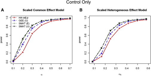
Power for Control-Only Analysis

Power results for control-only analysis $\left(n_0=700\right)$ from the (A) scaled common (homogeneous) effect data-generation model and (B) scaled heterogeneous effect data-generation model. Although the data were generated with an unstructured correlation matrix, three working correlation matrix structures for the joint outcome analyses were considered: I, independent; E, exchangeable; and U, unstructured. Power results were nearly identical with the use of I, E, and U for the 4-DF GEE tests, whereas power results were nearly identical with I and E, but not U, in the 1-DF SMAT; thus, only the results for GEE (U) and SMAT (E and U) are included.

Control + Affected Analysis

The empirical size results for the control + affected analyses are presented in the second and third columns of Table 3 and are quantitatively very similar to those from the control-only analyses, regardless of disease prevalence. The empirical sizes are close to the nominal values. Likewise, increasing the sample size to $n_0=n_1=1400$ results in more accurate size estimates (data not shown).

We present the power results for the scaled common effect data generation models assuming unstructured correlation (that is, generated with ${\mathbf{R}}^{\left(0\right)}={\mathbf{R}}^{\left(1\right)}\left(U\right)$ in Table 1) in Figure 2 for both the low (left column) and moderate (right column) disease prevalences and same (disease-independent; top row) and different (disease-dependent; bottom row) SNP effects for the affected and control individuals. For each plot, we see again that the 1-DF SMAT dominates in terms of power. Power is not sensitive to the presence of disease-dependent SNP effects as a consequence of the appropriate weighting.

Figure 2.

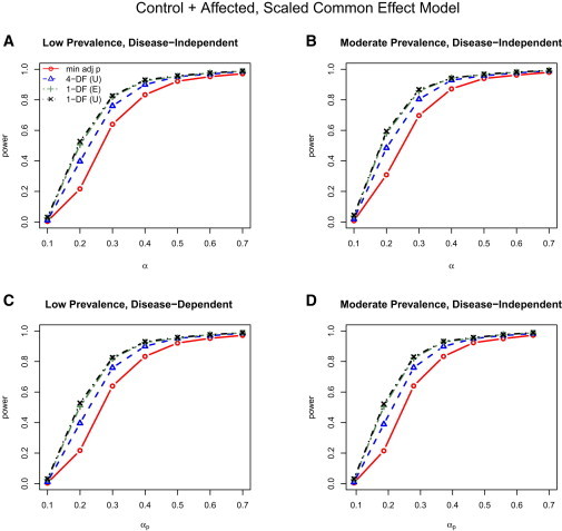
Power for Control + Affected Analysis under the Scaled Common Effect Model

Power results for control + affected analysis $\left(n_0=n_1=700\right)$ from the scaled common (homogeneous) effect data-generation model for both the low (left, A and C) and moderate (right, B and D) disease prevalences and same (top, A and B) and different (bottom, C and D) SNP effects for the affected and control individuals; that is, columns compare power with low $\left(\pi =0.000745\right)$ versus moderate $\left(\pi =0.0745\right)$ disease prevalences, and, thus, the effects of the weights, $w_i$, and rows compare power for disease-independent $\left({\alpha }^{\left(0\right)}={\alpha }^{\left(1\right)}\right)$ versus disease-dependent $\left({\alpha }^{\left(0\right)}\ne {\alpha }^{\left(1\right)}\right)$ SNP effects. Although the data were generated with an unstructured correlation matrix, three working correlation matrix structures for the joint outcome analyses were considered: I, independent; E, exchangeable; and U, unstructured. Power results were nearly identical with the use of I, E, and U for the 4-DF GEE tests, whereas power results were nearly identical with I and E, but not U, in the 1-DF SMAT; thus, only the results for GEE (U) and SMAT (E and U) are included.

Figure 3 displays the analogous plots for the scaled heterogeneous effect data generation model assuming unstructured correlation (that is, generated with ${\mathbf{R}}^{\left(0\right)}={\mathbf{R}}^{\left(1\right)}\left(U\right)$ in Table 1). As in the control-only simulation results (Figure 1B), the 1-DF SMAT still has higher power than both the 4-DF GEE and min-adj p tests, even when the scaled SNP effects are in fact heterogeneous. The gain in power experienced here, as well as in the scenario with true exchangeable correlation (that is, data generated with ${\mathbf{R}}^{\left(0\right)}={\mathbf{R}}^{\left(1\right)}\left(E\right)$ in Table 1) (data not shown), is due largely to the reduced degrees of freedom and moderate deviations from homogeneity under the scaled model.

Figure 3.

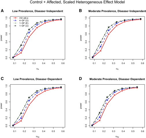
Power for Control + Affected Analysis under the Scaled Heterogeneous Effect Model

Power results for control + affected analysis $\left(n_0=n_1=700\right)$ from the scaled heterogeneous effect data-generation model for both the low (left; A, C) and moderate (right; B, D) disease prevalences and same (top; A, B) and different (bottom; C, D) SNP effects for the affected and control individuals; that is, columns compare power with low $\left(\pi =0.000745\right)$ versus moderate $\left(\pi =0.0745\right)$ disease prevalences, and, thus, the effects of the weights, $w_i$, and rows compare power for disease-independent $\left({\alpha }_j^{\left(0\right)}={\alpha }_j^{\left(1\right)},j=1,\dots ,4\right)$ versus disease-dependent $\left({\alpha }_j^{\left(0\right)}\ne {\alpha }_j^{\left(1\right)},j=1,\dots ,4\right)$. Although the data were generated with an unstructured correlation matrix, three working correlation matrix structures for the joint outcome analyses were considered: I, independent; E, exchangeable; and U, unstructured. Power results were nearly identical with the use of I, E, and U for the 4-DF GEE tests, whereas power results were nearly identical with I and E, but not U, in the 1-DF SMAT; thus, only the results for GEE (U) and SMAT (E and U) are included.

Subset of Phenotypes Associated with SNP

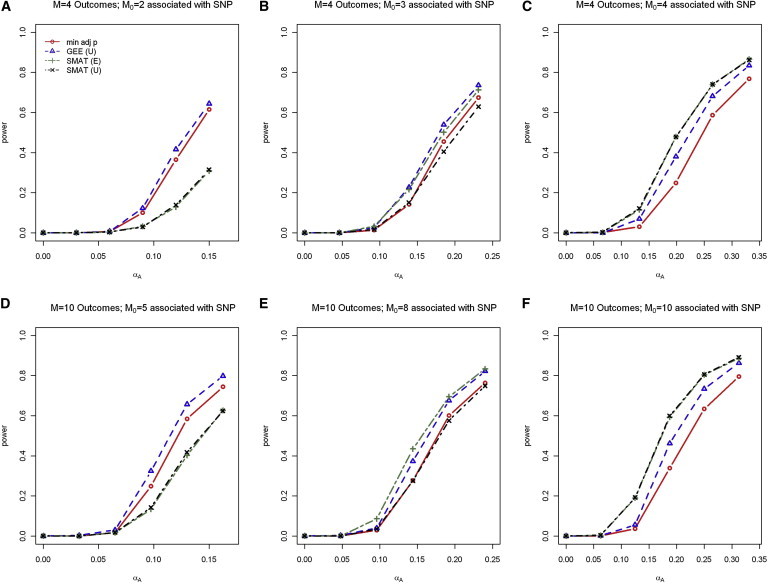
We present the power results for the situation where a subset of phenotypes is associated with SNP in Figure 4 for the control-only analysis. The results for control + affected analysis are similar and are included in the Supplemental Data (Figure S1). In these figures, the top (bottom) row displays the results for $M=4$ $\left(M=10\right)$ phenotypes for varying numbers of SNP-associated phenotypes, $M_0$. For a fixed sample size, we anticipated that the power of all tests would depend on a combination of factors, including the degree of correlation among phenotypes, the number of nonzero ${\alpha }_j$ (sparsity), and signal strength (magnitude) of nonzero ${\alpha }_j.$ For SMAT, the signal strength of nonzero ${\alpha }_j$ additionally influences heterogeneity among the scaled SNP effects.

Figure 4.

Power when a Subset of Phenotypes Are Associated with SNP

Power results for control-only analysis $\left(n_0=700\right)$ from the scaled heterogeneous effect model for $M=4$ phenotypes (A–C) and $M=10$ phenotypes (D–F) for various numbers of a subset of phenotypes associated with SNP $\left(M_0\right)$. Three working correlation matrix structures for the joint outcome analyses were considered: I, independent; E, exchangeable; and U, unstructured. Power results were nearly identical with the use of I, E, and U for the 4-DF GEE tests, whereas power results were nearly identical with I and E, but not U, in the 1-DF SMAT; thus, only the results for GEE (U) and SMAT (E and U) are included.

Our simulation results indicate that, when only 50% of the phenotypes are associated with SNP, SMAT has less power, and the M-DF GEE test is recommended. Note that, in this setting, the scaled common effect assumption under SMAT is strongly violated. For example, when $M_0=2$ and $M=4$, we conducted additional simulations to test for scaled homogeneity. For the last three power points, where the discrepancy between the methods is the greatest (${\alpha }_A$ near 0.10, 0.12, and 0.15), the sample median p values for the test of scaled homogeneity across 1,000 simulations are respectively 0.039, 0.005, and 0.0002, suggesting that the scaled homogeneity assumption is not satisfied in well over 50% of the simulated data sets at the 0.05 level.

When about 75% of the phenotypes are associated with SNP, SMAT has similar power to the M-DF GEE test when $M=4$ and has a higher power when $M=10$. In fact, when $M_0=3$ and $M=4$, our additional simulations for examining scaled homogeneity suggest for the last three power points (${\alpha }_A$ near 0.15, 0.20, and 0.25), again, where the discrepancy between the methods is the greatest, that the scaled common effect assumption is not satisfied in nearly 50% or more of the simulated data sets at the 0.05 level (sample median p values for test of homogeneity across 1,000 simulations are 0.059, 0.009, and 0.0008, respectively). In practice, it is desirable to check the scaled homogeneity assumption when using the SMAT test. When this assumption is strongly violated, the M-DF GEE test is recommended.

Interestingly, in these settings where some phenotypes are not associated with SNP, the SMAT method with the exchangeable and independent working correlation structures tends to be more powerful than SMAT with an unstructured working correlation structure. However, this is not unexpected. As with traditional GEE analysis, we would only expect an SMAT analysis with correctly specified correlation to yield the most efficient estimates when the mean model itself is correctly specified. When some phenotypes are not associated with SNP, the scaled common effect model misspecifies the true mean model more as the nonzero signal increases, and using the true correlation matrix (or unstructured working correlation matrix in this simulation) will not necessarily yield the most efficient estimates (that is, the smallest p values).

The plots in the right panel of Figure 4 compare the power when $M_0=M$; that is, all phenotypes are associated with SNP. As expected, SMAT is more powerful than the other methods.

Simulation: Test for Scaled Homogeneity

The tables and figures for the empirical size and power results for this set of simulations are included in the Supplemental Data. Note that only the results of the unstructured correlation matrix (see Table 1) are included. Table S1 indicates that the empirical size estimates for the estimating equation-based score test for homogeneity are preserved for both the control-only and control + affected analyses. Figures S2 and S3 display the power of the test for homogeneity as a function of (scaled) SNP effect heterogeneity across outcomes. As expected, as the SNP effect sizes become more heterogeneous, the power of the test to detect heterogeneity increases. An SD of true SNP effect sizes across outcomes of 0.1 yields approximately 80% power to detect heterogeneity at the 0.05 (type I error) level for the given sample size. However, it is important to note that, even when the scaled effects are moderately heterogeneous (that is, the null hypothesis of homogeneous scaled SNP effects may be rejected) but are in the same direction, the 1-DF scaled common effect test SMAT remains a powerful test (for example, see Figure 3).

GWAS on Smoking Behavior Results

Figure 5 displays the $-{\text{log}}_{10}$ p values for SMAT across all SNPs passing quality control. Manhattan plots for single-outcome analysis (unadjusted) p values are included in the Supplemental Data (Figures S4–S7). Quantile-quantile plots for the SMAT p values as well as the single-outcome analysis (unadjusted) p values are also included in the Supplemental Data (Figures S8 and S9). There were 13 SNPs from CDH18 that were nominally significant at $p<{10}^{-3}$ in at least one outcome. Two of these SNPs, rs4242066(C) and rs4461636(T) $\left(R^2>0.90\right)$, had p values $<{10}^{-5}$ in two outcomes; both had a negative relationship with duration and a positive relationship with cessation. Additionally, these same two SNPs had nominally significant p values in the other two outcomes; both had a positive relationship with initiation $\left(p<0.1\right)$ and a negative relationship with CPD $\left(p<0.001\right)$. The direction of the effects all correspond to less smoking. Similarly for CACNB2 (chromosome 10, MIM 600003), three SNPs on this gene were found nominally significant at $p<{10}^{-3}$ in at least one outcome, but only one of these SNPs, rs1277769(C), had p values $<{10}^{-3}$ in two outcomes (cessation and CPD). The directional relationships across the four outcomes and three SNPs were again all consistent with less smoking. These single-outcome results suggest that a joint 1-DF SMAT analysis may be advantageous for at least these SNPs, if not more.

Figure 5.

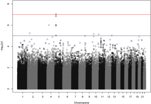
Manhattan Plot of Analysis of Multiple Smoking Behaviors

$-{\text{log}}_{10}$p values from the 1-DF scaled common effect test SMAT for all SNPs passing quality control. Analysis was performed on both affected $\left(n_1=696\right)$ and control $\left(n_0=730\right)$ ever-smokers with the use of $\pi =0.000745$ to determine the weights and an unstructured working correlation matrix.

There were 10 SNPs with p values $<{10}^{-5}$ with the 1-DF SMAT on the basis of the scaled common effect model, the smallest of which had a p value = 9.5 × 10⁻⁸; the same ten SNPs were identified in both the control-only and control + affected analyses (see Table 4). The p values for the 4-DF GEE test and the min-adj p test for the same ten SNPs are also provided for comparison. On the basis of the empirical correlation estimates (see, for example, Table 1), we chose to report the p values that resulted from using an unstructured working correlation matrix. However, p values obtained under the independent and exchangeable working correlation structures were of similar magnitudes.

We see several SNPs in Table 4 from CDH18 and one SNP from CACNB2. Indeed, the five SNPs identified from CDH18 are highly correlated with correlations in the range of $\left[0.69,0.97\right]$. Note that the two additional SNPs from CACNB2 from single-outcome analysis discussed above had p values $<{10}^{-4}$ from the 1-DF SMAT and are highly correlated with the CACNB2 SNP identified in Table 4. Additionally, SNPs from GEMIN6 (MIM 607006) and LHPP were also identified. As in the simulations, we see that the p values from the joint 1-DF SMAT analysis are smaller than those from the single-outcome-based min-adjusted p test and the 4-DF GEE test. For the ten SNPs identified, the p values for the test of homogeneity were all greater than 0.25, indicating that the common effect assumption is reasonable.

Moreover, SNPs from CDH18, CACNB2, and LHPP were identified before in at least one of three previously reported smoking cessation success clinical trials $\left(p<0.01\right)$²⁰. Among the ten SNPs listed in Table 4, there was weak evidence for SNP $\times$ gender interaction (unadjusted, individual $p<0.05$ for CPD) for only the SNPs from CDH18; stratified by gender, the estimates for SNP effect share same sign for both genders, but differ in magnitude with the association stronger for males.

Discussion

In this paper, we consider the analysis of multiple continuous secondary phenotypes in case-control studies. When multiple phenotypes measure the same underlying trait in the same direction (after transformation), we propose a powerful test, SMAT, for the common effect of a given SNP on multiple phenotypes using the scaled marginal model¹⁴ and use inverse probability-weighted estimating equations to adequately account for potential ascertainment bias induced by case-control sampling. This approach is robust to whether or not the secondary phenotypes are related to a primary disease outcome. In both simulation and data analyses, we demonstrate that, when the scaled effects of multiple phenotypes are homogeneous or moderately heterogeneous, the proposed 1-DF SMAT based on the scaled common effect model is more powerful than both the more traditional multivariate M-DF GEE test and the test with the single-outcome-based minimum p value adjusted for multiple comparisons.

Our approach allows one to account for arbitrary correlation among phenotypes and is also robust to the misspecification of the correlation among multiple phenotypes with the sandwich method. More power can be gained by correctly specifying the correlation among multiple phenotypes.

When multiple phenotypes measure the same underlying trait in the same biological direction (after transformations), one would expect that they are positively correlated. In this situation, the proposed that 1-DF SMAT is powerful for analyzing multiple (secondary) phenotypes in a range of scenarios when the scaled effects of multiple phenotypes are homogeneous or moderately heterogeneous. Specifically, the 1-DF SMAT is derived under the scaled common effect model. As expected, it is most powerful when the scaled common effect model holds. Furthermore, our results show that, when the scaled SNP effects on multiple outcomes are moderately heterogeneous, the 1-DF SMAT based on the scaled common effect model remains to have the correct size and a higher power than the multivariate M-DF test, assuming moderate heterogeneous SNP effects. In GWASs, given that the SNP effects are often small or moderate, it is reasonable to assume homogeneous or moderately heterogeneous SNP effects for scaled multiple continuous phenotypes, provided they measure the same underlying trait in the same direction (after transformation). This approach allows one to borrow information across multiple correlated phenotypes to increase test power, especially when SNP effects are weak, as in GWASs. Also, we proposed a scaled homogeneity test to assess the assumption of scaled homogeneous SNP effects. When a good portion of multiple phenotypes are not associated with SNP, the scaled homogeneity assumption (which can be tested with the scaled homogeneity test) is likely to be strongly violated, and the SMAT method might be less powerful; in these situations, the M-DF GEE test or individual phenotype analysis is recommended.

The proposed method can be also applied to studying pleiotropic effects. When modeling pleiotropic associations, in which loci are simultaneously associated with multiple phenotypes, to apply SMAT, it is desirable to first consider examining whether the multiple phenotypes biologically measure the same underlying trait or disease process in the same direction (after transformation); that is, if they are positively correlated after transformation. If not, or if they measure different underlying traits in different directions, or if a good proportion of phenotypes might not be associated with SNP, it is desirable to use the M-DF GEE test assuming heterogeneous SNP effects or simply analyze each phenotype separately for the improvement of power. To check this, one can simply calculate the sample correlation of multiple phenotypes or use biological knowledge. One can also perform the proposed scaled homogeneity test. In fact, for these scenarios, it might not be desirable to analyze multiple phenotypes simultaneously, because the results from the joint analysis might not be easily interpretable. Furthermore, when a large number of phenotypes are analyzed simultaneously, and if the majority of the phenotypes are not associated with a SNP, a multivariate M-DF GEE test could lose power compared to analyzing each phenotype separately.

In this paper, we focus on using the IPW method for analyzing multiple secondary phenotypes to correct for ascertainment bias in case-control studies where appropriate weights, $w_i$, determined on the basis of disease prevalence, are used. This approach is easy to implement and robust to the distributions of phenotypes. An alternative approach is to extend the retrospective likelihood methods¹² for multiple secondary phenotypes. Although this approach could potentially be more powerful than the proposed IPW approach, it is more complex and computationally intensive and is likely to be less robust in comparison to the proposed IPW method, given that a full likelihood and correct specification of the correlation among phenotypes is required. However, additional research is needed.

We applied our proposed methods to investigate SNP associations with multiple secondary smoking phenotypes and identified several SNPs of biological interest. Future research is needed to validate these findings. Recent large-scale GWASs (obtained by pooling data through meta analyses) and candidate gene studies for smoking behavior and nicotine dependence have identified several plausible genetic variants, an area on Chr15q24-25.1 being most consistently identified.^21–29 However, the effects identified in these published analyses were quite small and not detectable in the present analysis, most likely because of the limited sample size in our study (approximately 700 affected individuals and 700 control individuals).

The proposed method can be extended in a number of ways. Although the models considered in this work assume a common set of covariates, ${\mathbf{x}}_i$, for each outcome, the models can easily be modified to handle different sets of covariates for each outcome. We can also consider extending the model to handle multiple SNPs in a region; e.g., a gene, to potentially further improve power. Finally, it is also of interest to develop a similar framework for mixed outcome types (e.g., continuous and binary outcomes) if they measure the same underlying trait.

Appendix A: Unbiased Estimating Equations

In order to see that the estimating Equations 5 and 6 are indeed unbiased, let $I_S\left(i\right)$ be an indicator of individual i being sampled in a case-control data set from a cohort of size N. Clearly, $I_S\left(i\right)=1$ for all $n=n_0+n_1$ individuals in the case-control sample and 0 otherwise. The expectation of Equation 5 is given by

$$\begin{array}{c}E\left[\sum _{i=1}^n{w}_i{\mathbf{X}}_i^T{\mathbf{R}}^{-1}\left({\mathbf{y}}_i^{\text{*}}-{\mathbf{X}}_i\mathit{\gamma }\right)\right]=E\left[E\left\{\sum _{i=1}^N{I}_S\left(i\right)w_i{\mathbf{X}}_i^T{\mathbf{R}}^{-1}\left({\mathbf{y}}_i^{\text{*}}-{\mathbf{X}}_i\mathit{\gamma }\right)|D_i,{\mathbf{y}}_i,{\mathbf{X}}_i\right\}\right]\\ =\sum _{i=1}^{N}E\left[E\left\{I_S\left(i\right)w_i|D_i,{\mathbf{y}}_i,{\mathbf{X}}_i\right\}{\mathbf{X}}_i^T{\mathbf{R}}^{-1}\left({\mathbf{y}}_i^{\text{*}}-{\mathbf{X}}_i\mathit{\gamma }\right)\right]\\ =\frac{n}{N}\sum _{i=1}^{N}E\left[{\mathbf{X}}_i^T{\mathbf{R}}^{-1}\left({\mathbf{y}}_i^{\text{*}}-{\mathbf{X}}_i\mathit{\gamma }\right)\right]=0.\end{array}$$

The first equality follows from the definition of $I_S\left(i\right)$ and the law of iterated expectation. The penultimate equality results from the fact that $E\left\{I_S{w}_i|D_i,{\mathbf{y}}_i,{\mathbf{X}}_i\right\}=E\left\{I_S{w}_i|D_i\right\}=n/N$. This is because $E\left(I_S\left(i\right)=1|D_i\right)=Pr\left(I_S\left(i\right)=1|D_i\right)$, where $Pr\left(I_S\left(i\right)=1|D_i\right)$ is the conditional probability of individual i within the cohort being sampled, given disease status. Note that $Pr\left(I_S\left(i\right)=1|D_i=1\right)=n_1/\left(N\pi \right)=\left(n/N\right)\left(1/w_i\right)$ and $Pr\left(I_S\left(i\right)=1|D_i=0\right)=n_0/\left(N\left(1-\pi \right)\right)=\left(n/N\right)\left(1/w_i\right)$ for weight, $w_i$, defined in Equation 7. In other words, the weight, $w_i$, apart from a constant factor, is the inverse probability of individual i being sampled in the case-control sample. The final equality brings us to the cohort-based unbiased estimating equation of Roy et al.¹⁴

For Equation 6, denote ${\left[{\mathbf{X}}_i\mathit{\gamma }\right]}_j={\mathbf{x}}_i^T{\mathit{\beta }}_j+s_i\alpha$ for each j. Similarly, for each $j=1,\dots ,M$,

$$\begin{array}{c}E\left\{\sum _{i=1}^n{w}_i\left\{\frac{y_{ij}}{{\sigma }_j}\left(\frac{y_{ij}}{{\sigma }_j}-{\left[{\mathbf{X}}_i\mathit{\gamma }\right]}_j\right)-1\right\}\right\}=E\left\{E\left[\sum _{i=1}^N{I}_S\left(i\right)w_i\left\{\frac{y_{ij}}{{\sigma }_j}\left(\frac{y_{ij}}{{\sigma }_j}-{\left[{\mathbf{X}}_i\mathit{\gamma }\right]}_j\right)-1\right\}|D_i,{\mathbf{y}}_i,{\mathbf{X}}_i\right]\right\}\\ =\sum _{i=1}^{N}E\left[E\left\{I_S\left(i\right)w_i|D_i,{\mathbf{y}}_i,{\mathbf{X}}_i\right\}\left\{\frac{y_{ij}}{{\sigma }_j}\left(\frac{y_{ij}}{{\sigma }_j}-{\left[{\mathbf{X}}_i\mathit{\gamma }\right]}_j\right)-1\right\}\right]\\ =\frac{n}{N}\sum _{i=1}^{N}E\left[\left\{\frac{y_{ij}}{{\sigma }_j}\left(\frac{y_{ij}}{{\sigma }_j}-{\left[{\mathbf{X}}_i\mathit{\gamma }\right]}_j\right)-1\right\}\right]=0.\end{array}$$

Following similar arguments above, the final equality again brings us to the cohort-based unbiased estimating equation of Roy et al.¹⁴

Appendix B: Parameter Estimates and Their Standard Errors

After setting initial values for ${\mathit{\sigma }}^2$ and $\mathbf{R},$ we estimate $\mathit{\gamma }$ as

$${\mathit{\gamma }}_{new}={\left(\sum _{i=1}^n{w}_i{\mathbf{X}}_i^T{\mathbf{R}}^{-1}{\mathbf{X}}_i\right)}^{-1}\sum _{i=1}^n{w}_i{\mathbf{X}}_i^T{\mathbf{R}}^{-1}{\mathbf{y}}_i^{\text{*}}.$$

Given the current estimate of $\mathit{\gamma },$ we update the estimate of ${\mathit{\sigma }}^2$ using the Newton-Raphson (NR) method. Conveniently, terms required for the NR algorithm are also necessary for computation of the sandwich formula (see below for details) for the standard errors. Specifically, we have

$${\mathit{\sigma }}_{new}^2={\mathit{\sigma }}_{old}^2+{\left[\sum _{i=1}^n{w}_i\left\{{\mathbf{\Psi }}^{-1}+\frac{1}{2}diag\left({\mathbf{X}}_i\mathit{\gamma }\right){\mathbf{\Psi }}^{-1}diag\left({\mathbf{X}}_i\gamma \right)\right\}\right]}^{-1}\{\sum _{i=1}^n{w}_i\{{\mathbf{\Psi }}^{-1/2}diag\left({\mathbf{y}}_i\right)\left({\mathbf{y}}_i^{\text{*}}-{\mathbf{X}}_i\mathit{\gamma }\right)-1_{\mathbf{M}}\}\},$$

where $\mathbf{\Psi }=diag\left({\mathit{\sigma }}_{old}^2\right)$. The above updates are repeated until convergence.

For the estimation of the standard error of the parameters, denote the estimating equation of interest by $\mathbf{U}\left(\mathit{\delta }\right)={\sum }_{i=1}^n{\mathbf{U}}_i\left(\mathit{\delta }\right)=0$, where $\mathit{\delta }=\left({\mathit{\sigma }}^{2T},{\mathit{\gamma }}^T\right)$ and ${\mathbf{U}}_i={\left({\mathbf{U}}_{1i}^T,{\mathbf{U}}_{2i}^T\right)}^T$. Here, ${\mathbf{U}}_{1i}$ and ${\mathbf{U}}_{2i}$ correspond to the summands of Equations 6 and 5, respectively. Let $\hat{\mathit{\delta }}$ be the solution of $\mathbf{U}\left(\mathit{\delta }\right)=0.$ The variance of estimator $\hat{\mathit{\delta }}$ can be estimated as ${\mathcal{I}}^{-1}$, where $\mathcal{I}=\mathbf{H}{\left(\hat{\mathit{\delta }}\right)}^T{\left\{{\sum }_{i=1}^n{\mathbf{U}}_i\left(\hat{\mathit{\delta }}\right){\mathbf{U}}_i{\left(\hat{\mathit{\delta }}\right)}^T\right\}}^{-1}\mathbf{H}\left(\hat{\mathit{\delta }}\right)$ and

$$\mathbf{H}\left(\mathit{\delta }\right)=E\left(\frac{-\partial \mathbf{U}\left(\mathit{\delta }\right)}{\partial {\mathit{\delta }}^T}\right)=\left(\begin{array}{cc}{\mathbf{H}}_{11}& {\mathbf{H}}_{12}\\ {\mathbf{H}}_{21}& {\mathbf{H}}_{22}\end{array}\right),$$

with

$${\mathbf{H}}_{11}=\frac{1}{n}\sum _i{w}_i\left\{{\mathbf{\Psi }}^{-1}+\frac{1}{2}diag\left({\mathbf{X}}_i\mathit{\gamma }\right){\mathbf{\Psi }}^{-1}diag\left({\mathbf{X}}_i\mathit{\gamma }\right)\right\}{\mathbf{H}}_{12}=\frac{1}{n}\sum _i{w}_{i}diag\left({\mathbf{X}}_i\mathit{\gamma }\right){\mathbf{X}}_i$$

$${\mathbf{H}}_{21}=\frac{1}{2}\sum _i{w}_i{\mathbf{X}}_i^T{\mathbf{R}}^{-1}{\mathbf{\Psi }}^{-1}diag\left({\mathbf{X}}_i\mathit{\gamma }\right){\mathbf{H}}_{22}=\sum _i{w}_i{\mathbf{X}}_i^T{\mathbf{R}}^{-1}{\mathbf{X}}_i.$$

Appendix C: Score Test for the Assumption of Scaled Common Effect

Let ${\mathit{\gamma }}^0={\left({\mathit{\beta }}_1^T,\dots ,{\mathit{\beta }}_M^T,{\eta }_1\right)}^T,$ ${\mathit{\delta }}^0={\left({\mathit{\sigma }}^{2T},{\mathit{\gamma }}^{0T}\right)}^T,$ and $\mathit{\eta }={\left({\eta }_1,\dots ,{\eta }_M\right)}^T$ and partition the estimating functions as $\mathbf{U}\left(\mathit{\delta }\right)={\left({\mathbf{U}}^{1T},{\mathbf{U}}^{2T}\right)}^T$, where

$${\mathbf{U}}^1=\left(\begin{array}{c}\sum _i{w}_i{n}^{-1}\left\{{\mathbf{\Psi }}^{-1/2}diag\left({\mathbf{y}}_i\right)\left({\mathbf{y}}_i^{\text{*}}-{\mathbf{X}}_i{\mathit{\gamma }}^0-s_i{\text{Δ}}_1\mathit{\eta }\right)-1_{\mathbf{M}}\right\}\\ \sum _i{w}_i{\mathbf{X}}_i^T{\mathbf{R}}^{-1}\left({\mathbf{y}}_i^{\text{*}}-{\mathbf{X}}_i{\mathit{\gamma }}^0-s_i{\mathbf{\Delta }}_1\mathit{\eta }\right)\end{array}\right)$$ (Equation C1)

$${\mathbf{U}}^2=\sum _i{w}_i{s}_i\mathbf{\Lambda }{\mathbf{R}}^{-1}\left({\mathbf{y}}_i^{\text{*}}-{\mathbf{X}}_i{\mathit{\gamma }}^0-s_i{\text{Δ}}_1\mathit{\eta }\right),$$ (Equation C2)

where ${\mathbf{\Delta }}_j$ is the $M\times M$ identity matrix with the $j^{th}$ diagonal element replaced by 0, and $\mathbf{\Lambda }$ is an $\left(M-1\right)\times M$ matrix which is the identity matrix with the first row deleted. Note that Equation C1 is the estimating function for ${\mathit{\delta }}^0$, and ${\mathbf{U}}^2$ is the estimating function for ${\eta }_2,\dots ,{\eta }_M.$Using the results of Breslow³⁰, the score statistic

$$\text{S}={\left\{{\mathbf{U}}^2\left({\hat{\mathit{\delta }}}^{0T}\right)\right\}}^{T}co{v}^{-1}\left\{{\mathbf{U}}^2\left({\hat{\mathit{\delta }}}^0\right)\right\}{\mathbf{U}}^2\left({\hat{\mathit{\delta }}}^{0T}\right)$$

can be obtained easily, given that the computation of $cov\left\{{\mathbf{U}}^2\left({\hat{\mathit{\delta }}}^0\right)\right\}$ is a straightforward extension of the formulae in Roy et al.¹⁴ by accommodating the weights. Under the null hypothesis of common effect, the statistic, S, asymptotically follows a ${\chi }^2$ distribution with $M-1$ degrees of freedom.

Web Resources

The URLs for data presented herein are as follows:

• Online Mendelian Inheritance in Man (OMIM), http://www.omim.org

• R Package SMAT, http://www.hsph.harvard.edu/xlin/software.html

References

- 1.Manolio T.A., Collins F.S., Cox N.J., Goldstein D.B., Hindorff L.A., Hunter D.J., McCarthy M.I., Ramos E.M., Cardon L.R., Chakravarti A. Finding the missing heritability of complex diseases. Nature. 2009;461:747–753. doi: 10.1038/nature08494. [DOI] [PMC free article] [PubMed] [Google Scholar]
- 2.Hunter D.J., Kraft P., Jacobs K.B., Cox D.G., Yeager M., Hankinson S.E., Wacholder S., Wang Z., Welch R., Hutchinson A. A genome-wide association study identifies alleles in FGFR2 associated with risk of sporadic postmenopausal breast cancer. Nat. Genet. 2007;39:870–874. doi: 10.1038/ng2075. [DOI] [PMC free article] [PubMed] [Google Scholar]
- 3.Thomas G., Jacobs K.B., Yeager M., Kraft P., Wacholder S., Orr N., Yu K., Chatterjee N., Welch R., Hutchinson A. Multiple loci identified in a genome-wide association study of prostate cancer. Nat. Genet. 2008;40:310–315. doi: 10.1038/ng.91. [DOI] [PubMed] [Google Scholar]
- 4.Scott L.J., Mohlke K.L., Bonnycastle L.L., Willer C.J., Li Y., Duren W.L., Erdos M.R., Stringham H.M., Chines P.S., Jackson A.U. A genome-wide association study of type 2 diabetes in Finns detects multiple susceptibility variants. Science. 2007;316:1341–1345. doi: 10.1126/science.1142382. [DOI] [PMC free article] [PubMed] [Google Scholar]
- 5.Willer C.J., Speliotes E.K., Loos R.J., Li S., Lindgren C.M., Heid I.M., Berndt S.I., Elliott A.L., Jackson A.U., Lamina C., Wellcome Trust Case Control Consortium. Genetic Investigation of ANthropometric Traits Consortium Six new loci associated with body mass index highlight a neuronal influence on body weight regulation. Nat. Genet. 2009;41:25–34. doi: 10.1038/ng.287. [DOI] [PMC free article] [PubMed] [Google Scholar]
- 6.He C., Kraft P., Chen C., Buring J.E., Paré G., Hankinson S.E., Chanock S.J., Ridker P.M., Hunter D.J., Chasman D.I. Genome-wide association studies identify loci associated with age at menarche and age at natural menopause. Nat. Genet. 2009;41:724–728. doi: 10.1038/ng.385. [DOI] [PMC free article] [PubMed] [Google Scholar]
- 7.Lango Allen H., Estrada K., Lettre G., Berndt S.I., Weedon M.N., Rivadeneira F., Willer C.J., Jackson A.U., Vedantam S., Raychaudhuri S. Hundreds of variants clustered in genomic loci and biological pathways affect human height. Nature. 2010;467:832–838. doi: 10.1038/nature09410. [DOI] [PMC free article] [PubMed] [Google Scholar]
- 8.Diggle P.J., Heagerty P., Liang K.-Y., Zeger S.L. Oxford University Press; New York: 2002. Analysis of Longitudinal Data. [Google Scholar]
- 9.Monsees G.M., Tamimi R.M., Kraft P. Genome-wide association scans for secondary traits using case-control samples. Genet. Epidemiol. 2009;33:717–728. doi: 10.1002/gepi.20424. [DOI] [PMC free article] [PubMed] [Google Scholar]
- 10.Amos C.I., Wu X., Broderick P., Gorlov I.P., Gu J., Eisen T., Dong Q., Zhang Q., Gu X., Vijayakrishnan J. Genome-wide association scan of tag SNPs identifies a susceptibility locus for lung cancer at 15q25.1. Nat. Genet. 2008;40:616–622. doi: 10.1038/ng.109. [DOI] [PMC free article] [PubMed] [Google Scholar]
- 11.Hung R.J., McKay J.D., Gaborieau V., Boffetta P., Hashibe M., Zaridze D., Mukeria A., Szeszenia-Dabrowska N., Lissowska J., Rudnai P. A susceptibility locus for lung cancer maps to nicotinic acetylcholine receptor subunit genes on 15q25. Nature. 2008;452:633–637. doi: 10.1038/nature06885. [DOI] [PubMed] [Google Scholar]
- 12.Lin D.Y., Zeng D. Proper analysis of secondary phenotype data in case-control association studies. Genet. Epidemiol. 2009;33:256–265. doi: 10.1002/gepi.20377. [DOI] [PMC free article] [PubMed] [Google Scholar]
- 13.Rencher A.C. Second Edition. Wiley; New York: 2002. Methods for Multivariate Analysis. [Google Scholar]
- 14.Roy J., Lin X., Ryan L.M. Scaled marginal models for multiple continuous outcomes. Biostatistics. 2003;4:371–383. doi: 10.1093/biostatistics/4.3.371. [DOI] [PubMed] [Google Scholar]
- 15.Liang K.Y., Zeger S. Longitudinal data analysis using generalized linear models. Biometrika. 1986;73:13–22. [Google Scholar]
- 16.Hjsgaard S., Halekoh U., Yan J. The R Package geepack for Generalized Estimating Equations. J. Stat. Softw. 2005;15:1–11. [Google Scholar]
- 17.Vanderweele T.J., Vansteelandt S. Odds ratios for mediation analysis for a dichotomous outcome. Am. J. Epidemiol. 2010;172:1339–1348. doi: 10.1093/aje/kwq332. [DOI] [PMC free article] [PubMed] [Google Scholar]
- 18.Conneely K.N., Boehnke M. So many correlated tests, so little time! Rapid adjustment of P values for multiple correlated tests. Am. J. Hum. Genet. 2007;81:1158–1168. doi: 10.1086/522036. [DOI] [PMC free article] [PubMed] [Google Scholar]
- 19.Price A.L., Patterson N.J., Plenge R.M., Weinblatt M.E., Shadick N.A., Reich D. Principal components analysis corrects for stratification in genome-wide association studies. Nat. Genet. 2006;38:904–909. doi: 10.1038/ng1847. [DOI] [PubMed] [Google Scholar]
- 20.Rose J.E., Behm F.M., Drgon T., Johnson C., Uhl G.R. Personalized smoking cessation: interactions between nicotine dose, dependence and quit-success genotype score. Mol. Med. 2010;16:247–253. doi: 10.2119/molmed.2009.00159. [DOI] [PMC free article] [PubMed] [Google Scholar]
- 21.Saccone S.F., Hinrichs A.L., Saccone N.L., Chase G.A., Konvicka K., Madden P.A., Breslau N., Johnson E.O., Hatsukami D., Pomerleau O. Cholinergic nicotinic receptor genes implicated in a nicotine dependence association study targeting 348 candidate genes with 3713 SNPs. Hum. Mol. Genet. 2007;16:36–49. doi: 10.1093/hmg/ddl438. [DOI] [PMC free article] [PubMed] [Google Scholar]
- 22.Spitz M.R., Amos C.I., Dong Q., Lin J., Wu X. The CHRNA5-A3 region on chromosome 15q24-25.1 is a risk factor both for nicotine dependence and for lung cancer. J. Natl. Cancer Inst. 2008;100:1552–1556. doi: 10.1093/jnci/djn363. [DOI] [PMC free article] [PubMed] [Google Scholar]
- 23.Weiss R.B., Baker T.B., Cannon D.S., von Niederhausern A., Dunn D.M., Matsunami N., Singh N.A., Baird L., Coon H., McMahon W.M. A candidate gene approach identifies the CHRNA5-A3-B4 region as a risk factor for age-dependent nicotine addiction. PLoS Genet. 2008;4:e1000125. doi: 10.1371/journal.pgen.1000125. [DOI] [PMC free article] [PubMed] [Google Scholar]
- 24.Stevens V.L., Bierut L.J., Talbot J.T., Wang J.C., Sun J., Hinrichs A.L., Thun M.J., Goate A., Calle E.E. Nicotinic receptor gene variants influence susceptibility to heavy smoking. Cancer Epidemiol. Biomarkers Prev. 2008;17:3517–3525. doi: 10.1158/1055-9965.EPI-08-0585. [DOI] [PMC free article] [PubMed] [Google Scholar]
- 25.Furberg H., Kim Y., Dackor J., Boerwinkle E., Franceschini N., Ardissino D., Bernardinelli L., Mannucci P.L., Mauri F., Merlini P.A., Tobacco and Genetics Consortium Genome-wide meta-analyses identify multiple loci associated with smoking behavior. Nat. Genet. 2010;42:441–447. doi: 10.1038/ng.571. [DOI] [PMC free article] [PubMed] [Google Scholar]
- 26.Liu J.Z., Tozzi F., Waterworth D.M., Pillai S.G., Muglia P., Middleton L., Berrettini W., Knouff C.W., Yuan X., Waeber G., Wellcome Trust Case Control Consortium Meta-analysis and imputation refines the association of 15q25 with smoking quantity. Nat. Genet. 2010;42:436–440. doi: 10.1038/ng.572. [DOI] [PMC free article] [PubMed] [Google Scholar]
- 27.Thorgeirsson T.E., Gudbjartsson D.F., Surakka I., Vink J.M., Amin N., Geller F., Sulem P., Rafnar T., Esko T., Walter S., ENGAGE Consortium Sequence variants at CHRNB3-CHRNA6 and CYP2A6 affect smoking behavior. Nat. Genet. 2010;42:448–453. doi: 10.1038/ng.573. [DOI] [PMC free article] [PubMed] [Google Scholar]
- 28.Saccone N.L., Culverhouse R.C., Schwantes-An T.-H., Cannon D.S., Chen X., Cichon S., Giegling I., Han S., Han Y., Keskitalo-Vuokko K. Multiple independent loci at chromosome 15q25.1 affect smoking quantity: a meta-analysis and comparison with lung cancer and COPD. PLoS Genet. 2010;6:e1001053. doi: 10.1371/journal.pgen.1001053. [DOI] [PMC free article] [PubMed] [Google Scholar]
- 29.VanderWeele T.J., Asomaning K., Tchetgen Tchetgen E.J., Han Y., Spitz M.R., Shete S., Wu X., Gaborieau V., Wang Y., McLaughlin J. Genetic variants on 15q25.1, smoking, and lung cancer: an assessment of mediation and interaction. Am. J. Epidemiol. 2012;175:1013–1020. doi: 10.1093/aje/kwr467. [DOI] [PMC free article] [PubMed] [Google Scholar]
- 30.Breslow N. Tests of Hypotheses in Overdispersed Poisson Regression and Other Quasi-Likelihood Models. JASA. 1990;85:565–571. [Google Scholar]
Associated Data
This section collects any data citations, data availability statements, or supplementary materials included in this article.