Imaging dipole flow sources using an artificial lateral-line system made of biomimetic hair flow sensors

Abstract

In Nature, fish have the ability to localize prey, school, navigate, etc., using the lateral-line organ. Artificial hair flow sensors arranged in a linear array shape (inspired by the lateral-line system (LSS) in fish) have been applied to measure airflow patterns at the sensor positions. Here, we take advantage of both biomimetic artificial hair-based flow sensors arranged as LSS and beamforming techniques to demonstrate dipole-source localization in air. Modelling and measurement results show the artificial lateral-line ability to image the position of dipole sources accurately with estimation error of less than 0.14 times the array length. This opens up possibilities for flow-based, near-field environment mapping that can be beneficial to, for example, biologists and robot guidance applications.

1. Introduction

1.1. Sensor arrays

In Nature, animals can detect events in their environment with varying aptness, using different sources of sensory information. Having relevance to their survival, this information is used to find food, mate, avoid predators, etc. Many mammalian senses are found in arrays in which the integration of all sensors defines the function of the organ. Light receptors in the eye and chemosensory receptors in the nose and tongue are examples of such array systems.

Crickets [1], spiders [2], scorpions [3] and fish [4] all have flow sensory systems in the form of hair sensor arrays that detect tiny fluid movements. These biological sensor arrays are highly sensitive, very acute (e.g. with respect to directivity) and often possess a fair amount of redundancy, yielding a certain degree of robustness.

Lately, sensor arrays have become important research topics across disciplines with respect to smart sensory system developments [5,6]. Engineered sensor arrays contain a multiplicity of discrete sensor elements, each of which has a specific response to a specific stimulus. Based on the array task, the sensors can be arranged in, for example, planar or three-dimensional shapes. The array geometry and the sensors' positions (absolute or relative) are important design parameters and, in many applications such as antenna arrays, are a prerequisite for further processing of the array signals. In modern communications and radar systems, antenna arrays are essential for extracting weak signals from noisy backgrounds [7]. Using the overall available spatio-temporal array data, useful information related to the environment and objects in it may be extracted by integrating readings from multi-sensors in an appropriate manner while benefiting from array signal-processing (ASP) techniques. Examples of such embedded parameters, detected by array sensors, are direction of arrival (DoA) [8,9], number of sources estimation [6,10] and acoustic source localization [11].

1.2. Biomimetics

Recently, the concept of taking model systems from Nature (to attain new materials, fabrication techniques, devices and even entire systems) has been demonstrated to be a powerful route to improve upon more traditional engineering approaches for specific challenges. This so-called bio-inspired or biomimetic approach [12] may lead to unconventional designs that benefit from the optimization that the associated model system has attained over evolutionary time scales. Adapting principles and designs offered by Nature enables humans to better understand related phenomena and may help to surpass the performance of more traditional engineered systems.

1.3. Source localization

The estimation of object parameters using an array of sensors has been reported extensively in the literature. Being a highly interesting task, source localization has received great attention in ASP [13]. Tracking moving sources has many applications, including healthcare [5], satellite communication [14] and military purposes [15].

The methods for source localization that have been used intensively can be categorized into time delay estimation and beamforming [6]. The time delay method exploits the coherence between signals, as detected by various array elements, to extract information about the direction of the source. In beamforming, a full directional scan is performed, and the maximum signal power indicates the source direction. The appropriate signal-processing technique and associated complexity depend on the number of variables to be extracted and on the number of array elements and array configurations, for example linear-line array, uniform square array, circular array, etc.

In biomedical applications, several techniques take advantage of sensor arrays for source localization. The activities of the brain's neurons are recorded (electroencephalography) using arrays of electrodes and the number, position and strength of the neural sources are estimated [5]. Various skull models [16], signal models and signal-processing algorithms [5] have been developed and tested to improve source position estimation.

In radar and satellite applications, sensor arrays are used in target estimation processes. The goal is to determine various target parameters, for example location, velocity and size. Various array shapes, signal models and tracking algorithms have been developed and implemented to minimize system complexity and/or reduce estimation errors [14].

In robotic applications, arrays made of two microphones (mounted on a robot) have been used for DoA estimations [17]. The ratio of power spectrum amplitudes for two microphones was used as a feature vector, either with or without the use of the phase, and statistical pattern recognition was used to determine the direction of the source.

In sensor research, Nature offers a wide range of possibilities to improve performance of the traditional sensory systems. The biomimetic approach may include materials, sensing principles, sensory systems, detection mechanisms and computational algorithms inspired by biological models. Hearing in mammals and bats in particular, the lateral-line system (LLS) of fish, slit-sensilla-based localization in scorpions and airflow detection by hair-sensor-populated cercal arrays in crickets provide fascinating examples for engineers to imitate either in their hardware and/or in information processing. Inspired by bats, echolocation spectral analysis has been used to observe and localize features in realistic environments, i.e. walls and obstacles [18]. Reflector localization is based on the comparison of measured echoes with echo templates from different angles, and, hence, the shape and position of the surroundings are determined. The LLS in fish has been used as a source of inspiration in the fabrication of biomimetic, piezo-resistive flow sensor arrays using the plastic deformation magnetic assembly process [19]. The scorpion strategy is another example of source localization using sensor arrays. A biologically plausible prey localization scheme in scorpions has been presented and tested using a neuronal model [3]. In this model, the stimulus angle is determined, using the received excitatory input from one tarsus and the inhibition from a triad opposite to it.

2. Lateral-line system

In literature, specifically, the LLS has been the subject of extensive research in attempts to understand hydrodynamic imaging of the surroundings and source localization processes in fish [20]. The LLS is considered as a natural mechanosensory system where information can be drawn not only from the temporal features of a flow field but also from its spatial characteristics. It consists of spatially distributed neuromasts sensitive to fluid flow and arranged in a more or less linear array structure [4]. Each neuromast consists of several hair cells embedded together inside a jelly-like structure called a cupula. The LLS may contain both superficial neuromasts (SNs) and canal neuromasts (CNs) [21]. The SNs are located on the scales of the fish and are sensitive to fluid velocity, whereas the CNs are positioned inside canals beneath the skin and are sensitive to pressure gradients [4]. The combination of all flow signals is further processed to extract meaning from the detected flow fields rather than being just a collection of uncorrelated single point measurements, i.e. it allows for constructing flow images. These hydrodynamic images can be used to detect features and events in the environment, from the water flows and disturbances created by obstacles or probed by their self-generated flows. Figure 1 is a schematic of LLS in fish.

Figure 1.

Schematic of the LLS in fish. Composition adapted from Izadi [22] with scanning electron microscope image adapted from Hudspeth [23]. (Online version in colour.)

The function and operation of the LLS is not completely known but it is believed that with the LLS fish have the ability to sense their own movement, track positions of other animals within a distance proportional to their body length (with low-frequency range of 100 Hz or less), make sexual communications and avoid collisions (e.g. in schooling) [24–27]. Biologists and biophysicists are trying to understand the processes of source localization by the LSS through various hypotheses [28]. One of these hypotheses is based on observing the flow field generated by a harmonic dipole source and by determination of the characteristic points of the flow field. For example, the distance between a flow sensor array and a dipole source (i.e. source–LLS distance (D)) is encoded in the distance between these characteristic points.

A sphere vibrating parallel (//) with a linear array line, as indicated in figure 2, generates a flow velocity with components in the x- and y-directions with amplitude (here, we focus on the parallel field component [28,29])

2.1

where ω is the angular vibration frequency, a is the sphere radius, s is the sphere displacement amplitude and D is the distance between the centre of the sphere and sensor reference line (x-axis). Figure 2 shows a simulated example for the parallel component of a dipole field positioned at distance D as typical receptive field plots.

Figure 2.

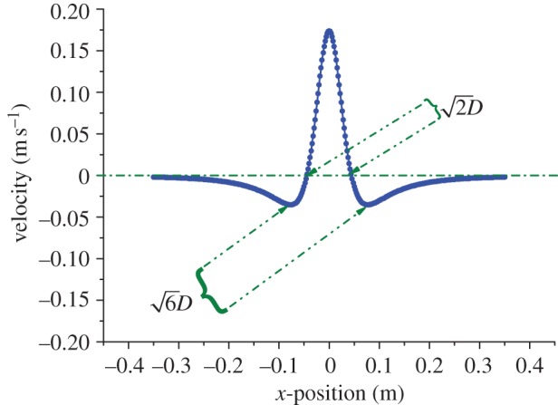
Simulated amplitudes of the parallel component (along the x-direction) for the velocity field of a dipole vibrating parallel with the x-axis as a function of the sensor position along the LLS (x-axis). The LLS to dipole-source distance (D) is encoded in the characteristic points of the dipole field (distance between zero-crossing points for the parallel component). The model presented in Goulet et al. [29] has been used to generate the data in this figure. For further information, see the electronic supplementary material. (Online version in colour.)

From figure 2, the parallel component of the dipole velocity profile is characterized by three peaks separated by two 180° phase shifts for the parallel component. The velocity components uniquely encode the distance to the source, irrespective of the fluid properties, vibration frequency, amplitude, direction and dimensions of the moving object [28,29]. Inspection of equation (2.1) shows that

• — the two x values for which V_x,//(x) = 0 are equal to

• — V_x,//(x) has three extrema: one maximum at x = 0 and two minima at

Hence, the distance D can be determined in various ways: for V_x,//, the distance between the two zeros equals and the distance between the two minima is.

Several attempts have been reported in the literature to make an artificial lateral-line system (ALLS) [19,30]. Fan et al. [19] have made an ALLS by fabricating hair flow sensors, using microelectromechanical systems (MEMS) technology. Franosch et al. [30] have developed an ALLS prototype with a single hot-thermistor anemometric sensor positioned onto an underwater robotic system. They experimentally showed its ability to avoid underwater objects by measuring the magnitude of flow velocity changes, which depends on the distance to an obstacle.

Using MEMS advancements, we developed artificial hair flow sensors imitating the hair sensor of crickets [31]. Artificial hair flow sensor arrays in combinations with ASP techniques can aid in performing flow pattern measurements and estimation of source parameters. In this study, we report our progress in imitating Nature using an ALLS to localize the position of a harmonic flow source, complementing our biomimetic scenario of using arrays of hair sensors. Such a system may be beneficial to biologists to understand unknown source localization mechanism(s) in fish as well as to engineers who seek to develop systems for imaging the surrounding environment and robotic guidance applications. This study differs from previous work [32] as it uses ASP and ALLS with discrete hair sensors for dipole-source localization.

3. Artificial hair sensor

In this study, we use an artificial hair flow sensor inspired by the flow-sensitive hairs of crickets [31]. Our sensor was fabricated using sacrificial polysilicon surface micromachining technology to form a suspended silicon nitride membrane with an approximately 1 mm long SU-8 hair on top. The axis of maximum sensitivity is tilted 45° relative to the x-axis of the device. Aluminium electrodes are integrated on top of the membrane forming capacitors with the bottom substrate (as a common electrode). Owing to the viscous drag torque acting on the hairs the membrane tilts, and consequently the capacitors on both halves of the sensor change equally but oppositely. These capacitive changes, representing the airflow surrounding the hair, are measured differentially, reducing disturbances that are common to both sides of the sensor.

Based on the differential capacitive design of our hair sensor, both sides of the differential capacitors ideally have equal capacitances when the membrane is in its equilibrium position. This results in a zero current flow into the common electrode of the hair sensor. On the other hand, when the hair is exposed to an external airflow, this results in capacitance changes. In combination with two mutually out-of-phase AC voltage sources (delivering the carrier signals), the differential changes in capacitance are converted into an amplitude-modulated (AM) voltage signal. A synchronous demodulation technique, which consists of a multiplier followed by a low-pass filter, is used to recover the original airflow signal from the AM signal. Figure 3 represents the structure of the mechanoreceptive sensory hair with its source of inspiration.

Figure 3.

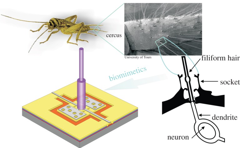
Schematic of flow sensors inspired by crickets. SEM close-up of a cricket's cercus, courtesy of Prof. J. Casas, Institut de Recherche sur la Biologie de l'Insecte, Tours, France. (Online version in colour.)

In the current hair sensor design, each hair flow sensor consisted of a group of 124 hairs with identical orientation and connected in parallel to increase the capacitance changes. Under ideal circumstances, i.e. identical hair flow sensors, no mutual mechanical (viscous) coupling and independent white noise, compared with a single-hair sensor, the resulting electrical signal is expected to be increased by a factor of 124, whereas the noise amplitudes are increased only by a factor of (124)^1/2, resulting in a signal-to-noise ratio (SNR) increase of about 11-fold. The maximum sensitivity axis of each individual hair is aligned at 45° relative to the long axis of the sensor die. A scanning electron microscope (SEM) image for part of the hair flow sensor illustrating grouping of hairs and the orientation angle of the maximum sensitivity axis is shown in figure 4.

Figure 4.

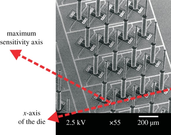
An SEM image of an artificial hair flow sensor of the previous generation. (Online version in colour.)

Previously, we have constructed an ALLS (inspired by the LLS of fish) using a single-hair flow sensor, and used it to localize the position of a dipole source (vibrating sphere) [32]. The motivation here is to develop an ALLS that mimics the retrieval of sensory information as obtained by the lateral line of fish and that provides the same possibilities for source localization (despite the fact that the mechanism of source localization in fish may be different). The ability of our hair flow sensors to measure the projection of the dipole flow field at positions along the ALLS is examined by the accuracy of localization of a vibrating dipole source. A vibrating sphere was used to represent the dipole source. The characteristic points of the dipole field were used in the source localization. The results show the ability of our ALLS to determine the dipole field at the position of the ALLS and to localize the position of a dipole source (vibrating sphere). However, this method has some limitations in the estimation of the source position when the flow source is not located alongside the ALLS. As the flow source is positioned at the edges or beyond the length of the ALLS, the characteristics of the flow field do not appear within the ALLS length and the estimation becomes impossible. Thus, for successful localization, the dipole source always has to be located alongside the ALLS. Additionally, if the zero-crossing of the perpendicular flow-field component is used to determine the lateral source position, then limited SNR causes large estimation errors. To overcome these limitations, different ASP techniques and algorithms have been considered to estimate the position of the dipole source. The use of some of these (beamforming) techniques can provide high-resolution source localization and is highly appreciated when the source is positioned at the edges of (or even beyond) the ALLS. The following sections provide some theory, modelling and implementation specifics of a beamforming technique as applied to the ALLS.

4. Beamforming

As part of ASP techniques, beamforming exploits the signal coming from one particular position as it impinges on all array sensors. This concept is used in various communication, voice and sonar applications [33]. The signal detected by each sensor is properly weighted, usually using model-based predictions, and the ensemble signals are used to determine the position of the source.

4.1. System model

Figure 5 shows a schematic of the ALLS used in combination with a beamforming technique for source localization. In this model, the vibrating sphere is the dipole source [34], and the sensor array is formed by artificial hair sensors positioned in a linear array shape constituting an ALLS similar to the lateral line in fish.

Figure 5.

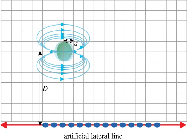
Schematic of the ALLS and its source of inspiration used for source localization with a beamforming technique. (Online version in colour.)

The current source-localization algorithm is based on calculation of a template based on anticipated array responses (equation (2.1); [29]) when a dipole source should be present at one of the many grid points within the area of interest (i.e. the dimension of the template matrix equals the number of grid points where each grid point is composed of a vector representing the array response). All other source parameters (e.g. direction, frequency and amplitude of vibration) were fed into the theoretical model (i.e. equation (2.1)) and the velocity amplitude represents its output. The goal is to generate a power image from the template matrix and the ALLS response vector, such that the position of maximum power corresponds with the most likely position of the source.

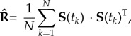
Once the dipole template is calculated for all possible source locations, the measured array response (S) is used to calculate an estimate of the sample covariance matrix by calculating the outer product of S according to equation (4.1) [35],

4.1

where k represents the sample number at time instant t_k and S^T is the transpose of S.

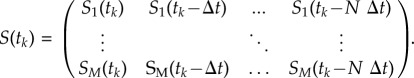
With M the number of hair sensors in the ALLS and N the number of samples, S is a matrix of M × N elements in which

4.2

The advantage is that the correlation matrix can be considered as a spatial filter that annihilates signals from positions where the source is not physically positioned [35]. The estimation accuracy of the covariance matrix can be improved and made less sensitive to noise when it is performed and averaged over N samples. The covariance matrix has M × M elements in which each single element represents the sum of the cross correlations between the sensor signals for different samples and with the autocorrelations at the diagonal of the matrix.

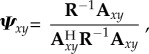
Once is computed, a beamforming technique based on Capon's algorithm [36,37] is used. The concept of this algorithm is that, for each position over the area of interest, a weighting vector (Ψ_xy) is applied to the sensor data. The Ψ_xy is determined in such a way that the optimal solution to recover the source signal owing to its position and to minimize the effect of noise and other positions will be [38]

4.3

where A_xy denotes the theoretical array response (steering vector) to a dipole source positioned at coordinates x,y as calculated from the source model in equation (2.1) and A^H is the Hermitian transpose of A.

The form of the ALLS response template at each grid point (x,y) will be a matrix of M × 1 elements in which

4.4

where V_M(x,y) represents the parallel velocity component of the dipole field (equation (2.1)) as an output of sensor number M owing to the source at grid point position (x,y).

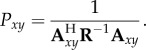
The associated output power (P_xy) at each grid point, where the source possibly could be, is calculated according to the following power weighting function [36,37]:

4.5

The resulting power level at each grid point is used to visualize the area of interest, i.e. the power map. The coordinates (x,y) of the maximum power level represent the most likely position of the dipole source.

4.2. Model performance

Modelling results under different conditions illustrate the application of the beamforming approach, based on Capon's algorithm, to the ALLS. The main target is determining a reliable estimate of the position of the source at varying positions and under different conditions. Figure 6 shows a successful localization of the dipole for two source positions within the area of interest. The results clearly show that, under favourable conditions, the hair array enables localization of the sphere position by beamforming, whether it is at the centre (figure 6a) or at the edges (figure 6b) of the ALLS. By contrast, using the methods described in §3 [32], the source is only traceable as long as the characteristic points of the flow field are positioned within the array boundaries.

Figure 6.

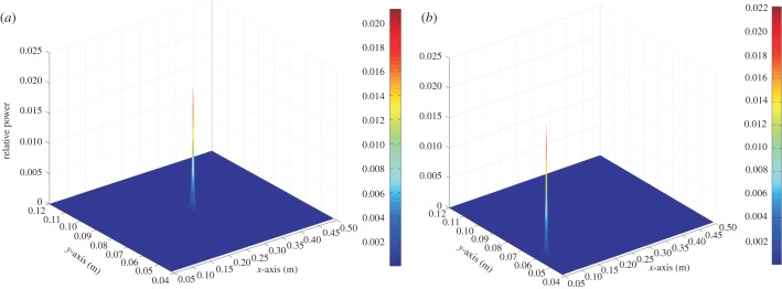
Dipole-source localization while the dipole source is positioned (a) at the array centre (X_pos = 0.275 m, Y_pos = 0.08 m) and (b) at the array edge (X_pos = 0.08 m, Y_pos = 0.06 m). Eight sensors were assumed to be positioned (relative to the origin (0,0)) at 0.1–0.45 m along the x-axis with 5 cm separation distance. For further information, see the electronic supplementary material.

5. Experimental set-up

We implemented and experimentally evaluated the performance of the ALLS (made of discrete artificial hair sensors), using beamforming techniques. A vibrating sphere (with a radius of 4 cm oscillating with amplitude of 3 mm at 40 Hz) was attached to a mini-shaker (PASCO model SF-9324) via a stainless steel shaft and used as a harmonic dipole source. The sphere position was controlled by a motorized dual-axis stage. The x-axis is defined as the direction parallel to the array, whereas the direction orthogonal to the array represents the y-axis. A linear array shape was constructed, using eight artificial hair flow sensors imitating the LLS (much like an array line of SNs). The array length (body length) was 0.35 m with 5 cm separation distance between array elements (eight sensors are positioned at 0.1–0.45 m relative to the (0,0) origin point). The maximum sensitivity axis for the hair sensors was aligned parallel to the dipole vibration axis to measure the parallel velocity field component. The direct digital synthesis system was used for generation of high-frequency (≈1 MHz) carrier signals in order to probe the hair sensors and to demodulate the generated AM signals from each of the array elements. The ALLS was subjected to a sinusoidal oscillating flow and aligned to localize the source in two dimensions (i.e. the x- and the y-positions). The measurements were carried out at a bandwidth of 300 Hz. A calibration process was conducted to exclude possible mismatches between individual array elements and, hence, the relative amplitudes are maintained (i.e. the maximum output signal of individual hair elements was measured, under the same conditions but for different hairs, and then the responses of individual hairs sensors were scaled with a factor to match the response of the hair which has the highest response). A theoretical model for the dipole source is used to estimate projections of the velocity pattern on the ALLS for each sphere position over the area of interest (needed to create the array response template A). The response of the ALLS was fed serially to a computer with 1 kHz rate data streams for further processing using the Matlab environment. The fast Fourier transform (FFT) amplitude of the sensor signal in windows of 256 samples was used to determine the signal amplitudes at the oscillation frequency of the sphere for each sensor channel. The beamforming technique (discussed in §4) is applied afterwards to the measurements, and a power map is generated for the area of interest. The coordinates with maximum power level predict the sphere position. Figure 7 shows a photograph of the experimental set-up for source localization using ALLS.

Figure 7.

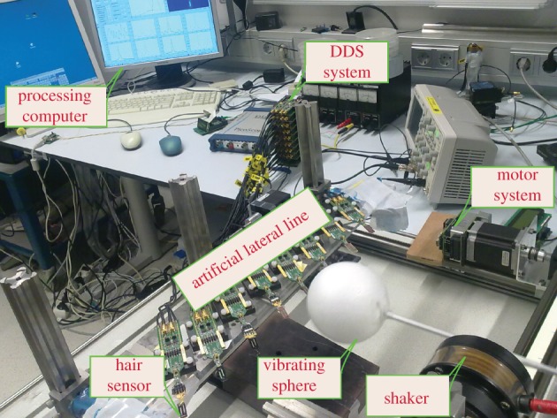
A photograph of the measurement set-up dedicated to source localization with beamforming.

6. Results

6.1. Offline measurements

Figure 8 shows a normalized representation of a dipole field measurement as detected by the ALLS compared with a normalized representation of the parallel component of the flow as given by the theoretical dipole field. The detected field matches satisfactorily with theoretical predictions and is used to localize the dipole source. Afterwards, the array responses were fed in an offline manner to the beamforming model discussed earlier. The results (figure 9) show the possibility of determining the dipole field components at the position of the hair sensor array, when arranged as an ALL. The accuracy of the field detection is examined by the amount of error in the source localization. Figure 9 illustrates the prediction of the dipole source position (for the data presented in figure 8), using the ALLS and the beamforming method.

Figure 8.

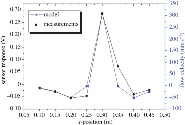
Dipole flow field measurements at the position of the hairs array (as detected by eight hair sensors at x = 0.3 m, D = 0.068 m) versus the theoretical model. For further information, see the electronic supplementary material. (Online version in colour.)

Figure 9.

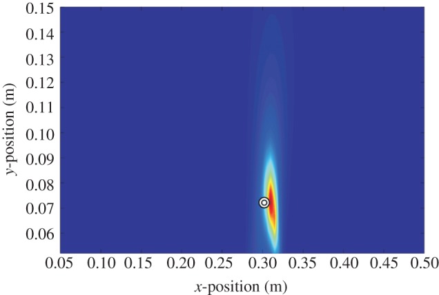
Dipole-source localization using ALLS. Source positioned at x = 0.3 m, D = 0.068 m (indicated by the circle) and the estimated position is x_est = 0.31 m, D_est = 0.072 m. The red area indicates the area of increased likelihood of the source position.

6.2. Online measurements

Inspired by the lateral-line function in fish, we demonstrated dipole-source localization using our hair sensors and Capon's method. A demonstrator was built, using the same offline experimental set-up. Eight measurements from the hair sensors were collected and processed online with FFT snapshots of 256 samples each. The dipole source was placed at different (x,y) positions along and from the ALLS. Each D_est was determined, using three measurements taken at the same D but at different x-positions along the ALLS (edges and centre). Afterwards, the average of D_est was calculated. Figure 10 shows a screen snapshot of the graphical user interface (GUI) of the demonstrator.

Figure 10.

Screen snapshot representing the GUI of the dipole-source localization demonstrator.

The performance of the demonstrator in terms of position estimation accuracy is assessed by comparison with the real physically measured distance values (D). The results show that the estimated distances between the sphere and the ALLS match the set distance reasonably well. Figure 11 shows D_est versus D, and figure 12 shows the estimation for the x-position of the dipole source along the array with their linear fit lines.

Figure 11.

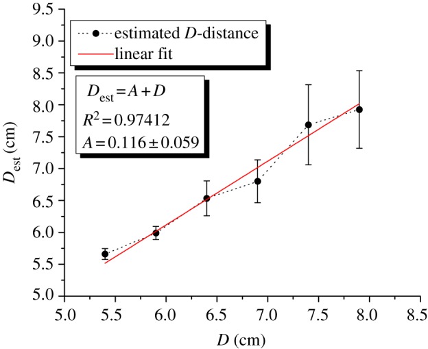
Dipole-source localization determined using the beamforming technique (dots) and linear fit between D and D_est (solid line). Error bars represent the standard error of the mean (i.e. the standard deviation of the samples used to determine the mean values). For further information, see the electronic supplementary material. (Online version in colour.)

Figure 12.

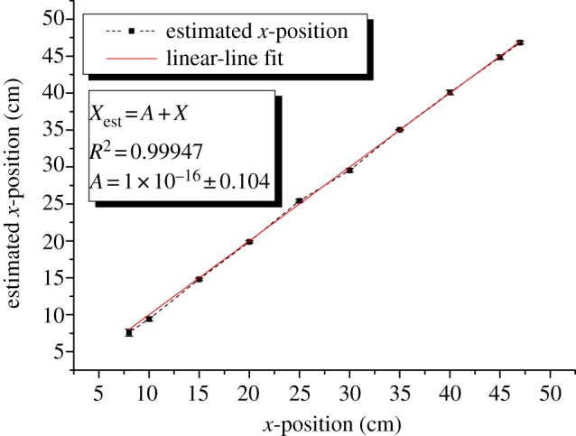
Near-linear relation between the actual and predicted x-position of the dipole source using beamforming techniques. Error bars represent the standard error of the mean. For further information, see the electronic supplementary material. (Online version in colour.)

7. Discussion

The abovementioned results verify the usability of artificial hair sensor arrays to localize dipole sources and can give insights into localization mechanisms in fish. However, D_est shows up to 0.17 cm shift from the set D. Estimation uncertainty can partially be attributed to the following factors that add additional uncertainty to D_est and cause deviation from the theoretical model:

• — Dissimilarities between individual ALLS elements, attributed to non-perfect matching even after calibration of the sensors is performed.

• — The constitution of the sensors (124 hairs over an area of 10 × 1 mm² connected in parallel to increase capacitance changes [39]) causes some blurring, affecting both the directivity and apparent position of the hair sensor.

• — Each D_est was determined using the average of three measurements taken at different x-positions along the ALLS (edges and centre). This causes uncertainty, because the estimation error increases when moving the dipole source from the centre to the edges of the ALLS (figure 13).

• — Here, the beamforming technique is performed using eight hair sensors with 5 cm separations in between. This limits the resolution of the measurements. We believe that increasing the number of sensors potentially improves the performance by providing higher resolution in the power images.

Figure 13.

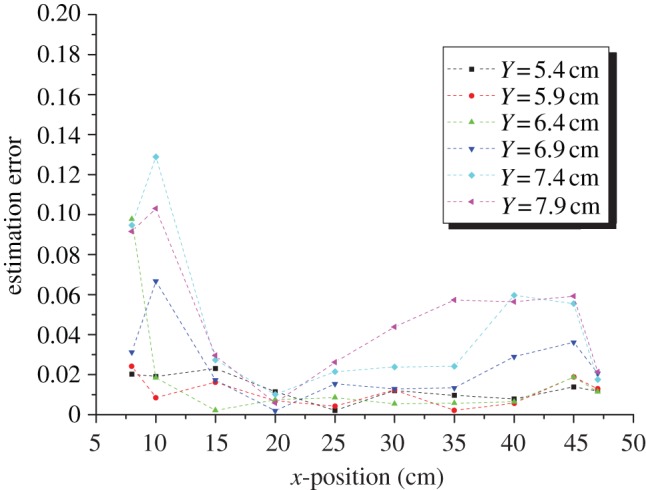
Source localization performance as a function of the source position relative to the ALLS. The absolute estimation error (error = [(D − D_est)² + (X − X_est)²]^1/2) is normalized to the body length of the ALLS, i.e. 0.35 m. For further information, see the electronic supplementary material.

On the other hand, the x-coordinate estimation shows better performance than the estimation of the y-coordinate (D). When compared with D_est, X_est shows up to 0.1 cm shift from the set X. We ascribe this to the large SNR for the sensors neighbouring the x-projection of the main peak of the dipole field (figure 8). Thus, its contribution in the cost function (equation (4.5)) is large compared with other sensor outputs along the ALLS (figure 12).

The overall array performance at different x–y coordinates is shown in figure 13, with its three-dimensional representation in figure 14. The array showed an ability to predict the position of the dipole source within and outside the dimensions of the ALLS with estimation errors of less than 0.14 body length at different distances of D. The estimation accuracy significantly improves to less than 0.02 body length when the sphere is positioned within the length of the ALLS. This clearly confirms the advantage of using such array-processing techniques over the characteristic points technique to localize the dipole source (see §3). Such capability of ALLS could shed some light on the spatial information processing in fish to image flow phenomena and assist engineers to design artificial systems to detect flow patterns or events, i.e. flow camera applications.

Figure 14.

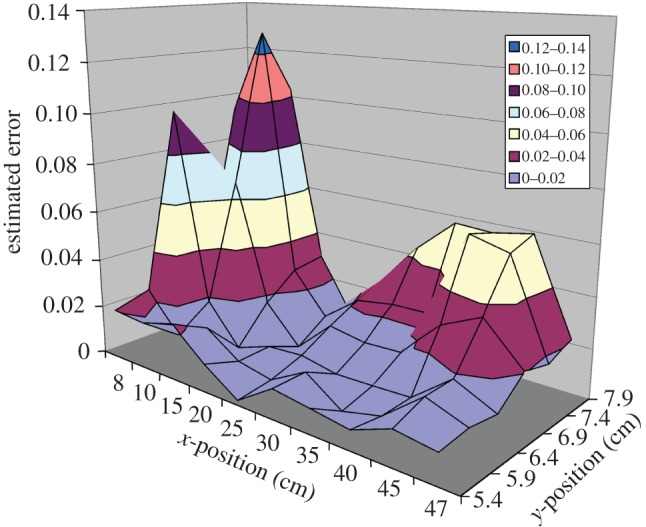
Three-dimensional representation of the source localization performance for the data presented in figure 13.

8. Conclusions and outlook

We showed the capability of the hair flow sensors to determine flow velocity of dipole fields. A linear array made up of eight artificial hair flow sensors was used to imitate the LLS in fish. ASP in combination with an ALLS shows the possibility to localize positions of dipole sources very well even at the edges or outside the ALLS length while maintaining high robustness.

Future studies will focus on modelling and implementing different array shapes and processing algorithms using single-die ALLS arrays. Additionally, simultaneous measurement of the parallel and perpendicular flow velocity components opens up possibilities of extracting more information about the source and, hence, better localization, especially for non-zero sensor-source angles. Once this is accomplished, pattern recognition techniques can be used to identify sources, phenomena and activities using spatial–temporal flow distributions. Such a system will assist biologists to understand the localization mechanisms in fish and engineers to use it in guiding robotic applications.

References

- 1.Shimozawa T, Murakami J, Kumagai T. 2003. Cricket wind receptors: thermal noise for the highest sensitivity known. In Sensors and sensing in biology and engineering (eds Barth FG, Humphrey JAC, Secomb TW.), pp. 145–157 Berlin, Germany: Springer [Google Scholar]
- 2.Albert JT, Friedrich OC, Denchant HE, Barth FG. 2001. Arthropod touch reception: spider hair sensilla as rapid touch detectors. J. Comp. Physiol. 187, 303–312 10.1007/s003590100202 (doi:10.1007/s003590100202) [DOI] [PubMed] [Google Scholar]
- 3.Sturzl W, Kempter R, van Hemmen JL. 2000. Theory of arachnid prey localization. Phys. Rev. Lett. 84, 5668–5671 10.1103/PhysRevLett.84.5668 (doi:10.1103/PhysRevLett.84.5668) [DOI] [PubMed] [Google Scholar]
- 4.Coombs S. 2001. Smart skins: information processing by lateral line flow sensor. Auton. Robots 11, 255–261 10.1023/A:1012491007495 (doi:10.1023/A:1012491007495) [DOI] [Google Scholar]
- 5.Yildiz G, Duru AD, Ademoglu A. 2007. A comparative study of localization approaches to EEG source imaging. In Proc. IEEE/NIH Life Science Systems and Applications Workshop, pp. 56–59 Bethesda, MD: LISA [Google Scholar]
- 6.Atmoko H, Tian DC, Tian GY, Fazenda B. 2008. Accurate sound source localization in a reverberant environment using multiple acoustic sensors. Meas. Sci. Technol. 19, 024003. 10.1088/0957-0233/19/2/024003 (doi:10.1088/0957-0233/19/2/024003) [DOI] [Google Scholar]
- 7.Viberg M, Ottersten B, Nehorai A. 1995. Performance analysis of direction finding with large arrays and finite data. IEEE Trans. Signal Process. 43, 469–477 10.1109/78.348129 (doi:10.1109/78.348129) [DOI] [Google Scholar]
- 8.Pirinen T, Yli-Hietanen J. 2004. Time delay based failure-robust direction of arrival estimation. In Proc. 3rd IEEE Sensors Array and Multichannel Signal Processing Workshop, Sitges, Spain, 18–21 July 2004, pp. 618–622 Washington, DC: IEEE. [Google Scholar]
- 9.Haupy RL. 2010. Antenna arrays: a computational approach. London, UK: John Wiley & Sons [Google Scholar]
- 10.Ishi CT, Chatot O, Ishiguro H, Hagita N. 2009. Evaluation of a MUSIC-based real-time sound localization of multiple sound sources in real noisy environments. In Proc. IEEE/RSJ Int. Conf. on Intelligent Robots and Systems, 2009 (IROS 2009), St. Louis, MO, 10–15 October 2009, pp. 2027, 2032. Washington, DC: IEEE. [Google Scholar]
- 11.Dowling EM, Linebarger DA, Tong Y, Munoz M. 1992. An adaptive microphone array processing system. Microprocess. Microsyst. 16, 507–516 10.1016/0141-9331(92)90080-D (doi:10.1016/0141-9331(92)90080-D) [DOI] [Google Scholar]
- 12.Vincent J. 2001. Stealing ideas from nature. In Deployable structures, ch. 3 (ed. Pellegrino E.), pp. 51–58 Vienna, Austria: Springer [Google Scholar]
- 13.Stark H, Woods JW. 2002. Probability and random processes with application to signal processing . Upper Saddle River, NJ: Pearson Education [Google Scholar]
- 14.Brandes TS, Benson RH. 2007. Sound source imaging of low-flying airborne targets with an acoustic camera array. Appl. Acoust. 68, 752–765 10.1016/j.apacoust.2006.04.009 (doi:10.1016/j.apacoust.2006.04.009) [DOI] [Google Scholar]
- 15.Navrátil M, Dostálek P, Křesálek V. 2010. Classification of audio sources using neural network applicable in security or military industry. In Proc. 2010 Int. Carnahan Conf. on Security Technology (ICCST), San Jose, CA, 5–8 October 2010, pp. 369–374 Washington, DC: IEEE. [Google Scholar]
- 16.Radich B, Buckley KM. 1994. Map estimation of EEG dipole source locations for head models with parameter uncertainty. In Proc. Statistical Signal and Array Processing, IEEE 7th SP Workshop, Quebec, Canada, 26–29 June 1994, pp. 413–416 Washington, DC: IEEE. [Google Scholar]
- 17.Mochiki N, Ogawa T, Kobayashi T. 2008. Ears of the robot: direction of arrival estimation based on pattern recognition using robot-mounted microphones. IEICE Trans. Inf. Syst. E91-D, 1522–1530 10.1093/ietisy/e91-d.5.1522 (doi:10.1093/ietisy/e91-d.5.1522) [DOI] [Google Scholar]
- 18.Reijniers J, Peremans H. 2007. Biomimetic sonar system performing spectrum-based localization. IEEE Trans. Robotics 23, 1151–1159 10.1109/TRO.2007.907487 (doi:10.1109/TRO.2007.907487) [DOI] [Google Scholar]
- 19.Fan Z, Chen J, Zou J, Bullen D, Liu C, Delcomyn F. 2002. Design and fabrication of artificial lateral line flow sensors. J. Micromech. Microeng. 12, 655–661 10.1088/0960-1317/12/5/322 (doi:10.1088/0960-1317/12/5/322) [DOI] [Google Scholar]
- 20.Blake BC, van Netten SM. 2006. Source location encoding in the fish lateral line canal. J. Exp. Biol. 209, 1548–1559 10.1242/jeb.02140 (doi:10.1242/jeb.02140) [DOI] [PubMed] [Google Scholar]
- 21.Dijkgraaf S. 1963. The functioning and significance of the lateral-line organs. Biol. Rev. 38, 51–105 10.1111/j.1469-185X.1963.tb00654.x (doi:10.1111/j.1469-185X.1963.tb00654.x) [DOI] [PubMed] [Google Scholar]
- 22.Izadi N. 2011. Bio-inspired MEMS aquatic flow sensor arrays. PhD thesis, University of Twente, Enschede, The Netherlands [Google Scholar]
- 23.Hudspeth AJ. 2005. How the ear's works work: mechanoelectrical transduction and amplification by hair cells. C. R. Biol. 328, 155–162 10.1016/j.crvi.2004.12.003 (doi:10.1016/j.crvi.2004.12.003) [DOI] [PubMed] [Google Scholar]
- 24.Russell IJ. 1976. Amphibian lateral line receptors. In Frog neurobiology: a handbook (eds Llinas R, Precht W.), pp. 513–550 Berlin, Germany: Springer [Google Scholar]
- 25.Hassan ES. 1985. Mathematical analysis of the stimulus for the lateral line organ. Biol. Cybern. 52, 23–36 10.1007/BF00336932 (doi:10.1007/BF00336932) [DOI] [PubMed] [Google Scholar]
- 26.Coombs S, Fay RR. 1993. Source level discrimination by the lateral line system of the mottled sculpin, Cottus bairdi. J. Acoust. Soc. Am. 93, 2116–2123 10.1121/1.406672 (doi:10.1121/1.406672) [DOI] [PubMed] [Google Scholar]
- 27.Coombs S, Finneran JJ, Conley RA. 2000. Hydrodynamic image formation by the peripheral lateral line system of the Lake Michigan mottled sculpin, Cottus bairdi. Phil. Trans. R Soc. Lond. B 355, 1111–1114 10.1098/rstb.2000.0649 (doi:10.1098/rstb.2000.0649) [DOI] [PMC free article] [PubMed] [Google Scholar]
- 28.Franosch J-MP, Sichert AB, Suttner MD, van Hemmen JL. 2005. Estimating position and velocity of a submerged moving object by the clawed frog Xenopus and by fish. Biol. Cybern. 93, 231–238 10.1007/s00422-005-0005-0 (doi:10.1007/s00422-005-0005-0) [DOI] [PubMed] [Google Scholar]
- 29.Goulet J, Engelmann J, Chagnaud BP, Franosch J-MP, Suttner MD, van Hemmen JL. 2008. Object localization through the lateral line system of fish: theory and experiment. J. Comp. Physiol. 194, 1–17 10.1007/s00359-007-0275-1 (doi:10.1007/s00359-007-0275-1) [DOI] [PubMed] [Google Scholar]
- 30.Franosch J-MP, Sosnowski S, Chami NK, Kühnlenz K, Hirche S, van Hemmen JL. 2010. Biomimetic lateral-line system for underwater vehicles. In Proc. 9th IEEE Sensors Conference, Waikoloa, HI, 1–4 November 2010, pp. 2212–2217 Washington, DC: IEEE. [Google Scholar]
- 31.Krijnen GJM, Dijkstra M, van Baar JJ, Shankar SS, Kuipers WJ, De Boer RJH, Altpeter D, Lammerink TSJ, Wiegerink R. 2006. MEMS based hair flow-sensors as model systems for acoustic perception studies. Nanotechnology 17, S84–S89 10.1088/0957-4484/17/4/013 (doi:10.1088/0957-4484/17/4/013) [DOI] [PubMed] [Google Scholar]
- 32.Dagamseh AMK, Lammerink TSJ, Kolster ML, Bruinink CM, Wiegerink RJ, Krijnen GJM. 2010. Dipole-source localization using biomimetic flow-sensor arrays positioned as lateral-line system. Sens. Actuators A, Phys. 162, 355–360 10.1016/j.sna.2010.02.016 (doi:10.1016/j.sna.2010.02.016) [DOI] [Google Scholar]
- 33.Krim H, Viberg M. 1996. Two decades of array signal processing research: the parametric approach. IEEE Signal Process. Mag. 13, 67–94 10.1109/79.526899 (doi:10.1109/79.526899) [DOI] [Google Scholar]
- 34.Harris G, van Bergeijk W. 1962. Evidence that the lateral-line organ responds to near-field displacements of sound source in water. J. Acoust. Soc. Am. 34, 1831–1841 10.1121/1.1909138 (doi:10.1121/1.1909138) [DOI] [Google Scholar]
- 35.Qureshi TR, Van Veen BD. 2007. Effects of correlation matrix estimation on correlated source cancellation in beamformers. Int. Congr. Ser. 1300, 261–264 10.1016/j.ics.2006.12.057 (doi:10.1016/j.ics.2006.12.057) [DOI] [Google Scholar]
- 36.Capon J. 1969. High-resolution frequency-wavenumber spectrum analysis. Proc. IEEE 57, 1408–1418 10.1109/PROC.1969.7278 (doi:10.1109/PROC.1969.7278) [DOI] [Google Scholar]
- 37.Stoica P, Handel P, Soderstorm T. 1995. Study of capon method for array signal processing. Circuits Syst. Signal Process. 14, 749–770 10.1007/BF01204683 (doi:10.1007/BF01204683) [DOI] [Google Scholar]
- 38.Lorenz RG, Boyd SP. 2005. Robust minimum variance beamforming. IEEE Trans. Signal Process. 53, 1684–1696 10.1109/TSP.2005.845436 (doi:10.1109/TSP.2005.845436) [DOI] [Google Scholar]
- 39.Dagamseh AMK, Bruinink CM, Droogendijk H, Wiegerink RJ, Lammerink TSJ, Krijnen GJM. 2010. Engineering of biomimetic hair-flow sensor arrays dedicated to high-resolution flow field. In Proc. 9th IEEE Sensors Conference, Waikoloa, HI, 1–4 November 2010, pp. 2251–2254 Washington, DC: IEEE. [Google Scholar]