Monte Carlo methods for localization of cones given multielectrode retinal ganglion cell recordings

Abstract

It has recently become possible to identify cone photoreceptors in primate retina from multi-electrode recordings of ganglion cell spiking driven by visual stimuli of sufficiently high spatial resolution. In this paper we present a statistical approach to the problem of identifying the number, locations, and color types of the cones observed in this type of experiment. We develop an adaptive Markov Chain Monte Carlo (MCMC) method that explores the space of cone configurations, using a Linear-Nonlinear-Poisson (LNP) encoding model of ganglion cell spiking output, while analytically integrating out the functional weights between cones and ganglion cells. This method provides information about our posterior certainty about the inferred cone properties, and additionally leads to improvements in both the speed and quality of the inferred cone maps, compared to earlier “greedy” computational approaches.

Introduction

The retina is among the neural systems to which we have the best experimental access. On one hand, we can present stimuli at a fine enough resolution to simultaneously and individually excite all the photoreceptors in a wide area. On the other hand, we can simultaneously record from and sort the spikes of nearly all the ganglion cells of certain types within a region spanning hundreds of ganglion cells (Chichilnisky and Kalmar 2002; Segev et al. 2004; Frechette et al. 2005; Gauthier et al. 2009). We also have straightforward phenomenological models which can predict the spiking output of these ganglion cells types in response to random white noise stimuli with reasonable accuracy (Chichilnisky 2001); Keat et al. 2001; Pillow et al. 2005; Pillow et al. 2008). To move forward in building more accurate models of the retina and understanding its function, we are at a stage where it is useful to identify individual cells involved in transducing the signal before it reaches the ganglion cell level.

A milestone in this direction was recently described in (Field et al. 2010), who showed that it is possible to identify individual cone photoreceptors given the spiking of multiple simultaneously recorded ganglion cells. Given sufficiently high resolution random stimuli, it was observed that the spike triggered averages (STA) of ganglion cells are made up of small islands of light sensitivity which overlap across different ganglion cells and are similar in shape, size and color to cone receptive fields. By comparing the locations of these islands of sensitivity with images of the cone layer from the same experiments, it was established that the small islands making up STAs are in fact individual cone receptive fields.

A typical multi-electrode experiment will gather spikes from hundreds of ganglion cells, whose STAs, covering different areas of the field of view, can be more or less sharp and informative about cone locations, depending on the number of spikes that were sorted and the characteristics of each ganglion cell. Thus for any experiment, the evidence pinpointing the locations of cones will be strong in some regions, while in other regions it may be hard to distinguish the underlying signal from noise in the estimated STA.

This work describes a statistical method for inferring cone locations and types, along with measures of confidence we can have in each inferred cone. We build upon the model and methods used in (Field et al. 2010), but utilize Markov Chain Monte Carlo (MCMC) computational inference methods (Robert and Casella 2005) instead of the simpler greedy optimization approach used in (Field et al. 2010). In addition to providing measures of posterior confidence in our inferred results, we find that the MCMC approach obtains cone maps of higher likelihood (demonstrating that the greedy approach is prone to local optima in this setting); we also note that a "lazy" implementation of the approach leads to a faster solution than the greedy method.

Experimental methods summary

The same protocols as in (Field et al. 2010) were used to collect similar data. Extracellular multi-electrode recordings were obtained from ganglion cells of isolated retinas taken from macaque monkeys (Macaca fascicularis and Macaca mulatta) used in other laboratories (Chichilnisky and Baylor 1999). Spikes from several hundred cells were segregated offline (Litke et al. 2003). Receptive-field maps were obtained using a fine grained random colored checkerboard stimulus projected onto the retina. Most importantly, pixel sizes were chosen to be smaller than cone receptive field sizes, for sufficient spatial resolution.

Linear-nonlinear Poisson hierarchical model

We model all the ganglion cells whose spikes were recorded simultaneously during an experiment jointly, with each cell indexed by i; in particular, the set of cones we infer is shared by all the ganglion cells of an experiment. However, to keep our notation simple, we start by suppressing i and focus on a single ganglion cell. As in (Field et al. 2010), we model each ganglion cell as a Linear-Nonlinear-Poisson (LNP) spike generator, with an exponential nonlinearity:

$$n_t~\mathit{\text{Poiss}}[e^{b+\mathbf{k}.{\mathbf{s}}_t}\mathrm{d}t]$$

We use the following notations:

st	the stimulus at time t.
T	length of the experiment, in time bins.
nt	spike train of the ganglion cell, discretized into spike counts per time bin.
b ∈ ℝ	an offset parameter that sets the neuron's baseline firing rate.
k	the ganglion cell's receptive field, a linear filter acting on the stimulus st.
k.st	the dot product of the ganglion cell's receptive field with the stimulus.
Nspikes	the total number of spikes recorded from the ganglion cell.
$\mathbf{\text{STA}}=\frac{1}{N_{\mathit{\text{spikes}}}}{\sum }_t{\mathit{n}}_t{s}_t$	the spike triggered average of the ganglion cell.

All of these quantities except for s_t and T are specific to a particular ganglion cell; they will all later be subscripted with ganglion cell number i.

The raw stimulus at time t and the raw STA have one temporal and two spatial dimensions. However, in these experiments ganglion cell receptive fields can be approximated as being separable in space and time (see (Chichilnisky and Kalmar 2002) for further discussion), and their temporal profile is easily obtained from the singular value decomposition of STA as in (Gauthier et al. 2009) (see Appendix). Since our cone finding problem is essentially spatial in nature, to simplify calculations we start by integrating out this temporal dimension in a preprocessing step (Gauthier et al. 2009). In our notation, both the stimulus s_t at time t and the STA of each ganglion cell only have two spatial dimensions (as well as one color dimension): the temporal dimension has been integrated out, so that s_t represents an effective filtered stimulus that represents the recent history of the presented visual stimulus. See the appendix for full details.

Under an LNP model, the log-likelihood of seeing spike train {n_t} given stimulus s_t and parameters b and k is

$$\text{log}p(\{n_t\left\}\right|b,\mathbf{k},{\mathbf{s}}_t)=\sum _{t=1}^T{n}_t(b+\mathbf{k}.{\mathbf{s}}_t)-e^{b+\mathbf{k}.{\mathbf{s}}_t}\mathrm{d}t+\mathit{\text{const}}.=N_{\mathit{\text{spikes}}}(b+\mathbf{k}.\mathbf{\text{STA}})-\sum _t{e}^{b+\mathbf{k}.{\mathbf{s}}_t}\mathrm{d}t+\mathit{\text{const}}.$$

Models of this type are well known and have been shown (Chichilnisky 2001) to be adequate for macaque parasol ganglion cells given low-to-moderate effective contrast, as defined by the standard deviation of the dot product k.s_t. Note however that more elaborate models that include spike history couplings between ganglion cells have been shown to be more appropriate for high-contrast stimuli (Pillow et al. 2008) (see also (Keat et al. 2001; Pillow et al. 2005)). Since our stimulus has such small pixels, the receptive fields k cover many pixels, so that the effective contrast, which averages the stimulus variability over all of k, is low enough here that spike history terms could be ignored. As discussed in the next section, this permitted the use of some approximations that were extremely helpful in speeding the computation.

Approximate profile log-likelihood

We begin with two key approximations of the loglikelihood:

$$\text{log}p(\{n_t\left\}\right|b,\mathbf{k},{\mathbf{s}}_t)\approx N_{\mathit{\text{spikes}}}(b+\mathbf{k}.\mathbf{\text{STA}})-T\int e^{b+\mathbf{k}.\mathbf{s}}p(\mathbf{s})\mathrm{d}\mathbf{s}+\mathit{\text{const}}.=N_{\mathit{\text{spikes}}}(b+\mathbf{k}.\mathbf{\text{STA}})-T\int e^{b+\mathbf{k}.\mathbf{s}}p(\mathbf{k}.\mathbf{s})\mathrm{d}(\mathbf{k}.\mathbf{s})+\mathit{\text{const}}.$$ (1)

$$\approx N_{\mathit{\text{spikes}}}(b+\mathbf{k}.\mathbf{\text{STA}})-T\int e^{b+\mathbf{k}.\mathbf{s}}{𝓅}_{\mathit{\text{gauss}}}(\mathbf{k}.\mathbf{s})\mathrm{d}(\mathbf{k}.\mathbf{s})+\mathit{\text{const}}.$$ (2)

$$=N_{\mathit{\text{spikes}}}(b+\mathbf{k}.\mathbf{\text{STA}})-T\exp (b+\frac{{\sigma }^2}{2}{\Vert \mathbf{k}\Vert }^2)+\mathit{\text{const}}.$$ (3)

The first approximation replaces a sum over experimental time bins with an integral over the stimulus distribution, which becomes an equality in the limit of infinite experimental time T. See (Paninski 2004); Park and Pillow 2011; Ramirez and Paninski 2012) for further discussion of this approximation. The second equation follows from the fact that the resulting integral only depends on the probability distribution of the one-dimensional projection k.s. The approximation in the third line is an application of the central limit theorem: sincek.s is a large weighted sum over many random variables (each element of the vector s in these experiments is independent, with mean zero and variance σ²; the weights are given by k), we can expect the distribution of k.s to be approximately Gaussian (with mean zero and variance ${\sigma }^2{\Vert \mathbf{k}\Vert }_2^2$) for all receptive fields k with a sufficiently large number of nonzero pixels. (See (Diaconis and Freedman 1984) for further discussion.) The final equality follows by analytically evaluating this Gaussian integral. (Note that this integral is not analytically available if spike history coupling terms are included in the model; see (Ramirez and Paninski 2012) for further discussion.)

Note that this sequence of approximations entails a huge computational savings, since once the STA and number of spikes N_spikes are obtained, we can discard the stimuli s_t and spikes {n_t} completely; in statistical language, the STA and N_spikes form an approximately sufficient statistic. Since the stimulus set is huge here (both in space, due to the high spatial resolution and in T, because long experiments are required to collect enough data to adequately constrain the cone inference), this approximation makes the computation orders of magnitude more efficient.

We can simplify further if we note that it is possible to optimize for the offset parameter b in (3) analytically, as a function of k:

$$\widehat{b}=\text{log}\frac{N_{\mathit{\text{spikes}}}}{T}\frac{{\sigma }^2}{2}{\Vert \mathbf{k}\Vert }_2^2.$$ (4)

Plugging this back into (3) results in a rather dramatic simplification:

$$\frac{1}{N_{\mathit{\text{spikes}}}}\text{log}𝓅(\{n_t\left\}\right|\mathbf{k},\mathbf{\text{STA}})\approx \mathbf{k}.\mathbf{\text{STA}}-\frac{{\sigma }^2}{2}{\Vert \mathbf{k}\Vert }^2+\mathit{\text{const}}.$$

In the statistical literature, this partially-maximized likelihood is often referred to as a “profile” likelihood; the key conclusion here is that the profile loglikelihood can be well- approximated as quadratic. The resulting approximately Gaussian likelihood will allow us to analytically integrate out the functional connectivity weights a between cones and ganglion cells that will be introduced in the next section.

If we do not impose any constraints, structure or regularization on the linear filter k, then maximizing the likelihood would result in k being proportional to the STA; this becomes apparent by equating the gradient of (3) with respect to k to zero (Paninski et al. 2004; Park and Pillow 2011). In this setting, we could write k = αSTA and solve for the unknown α which maximizes the profile likelihood, leading to α̂ = 1 lσ². In the following, the linear filter k will be constructed from cone receptive fields, and it will therefore not be strictly proportional to the STA. However, the approximation ∥STA∥σ² for the norm of k will continue to be useful below.

Weighted sums of cone receptive fields

We now assume that each ganglion cell’s linear filter k is a weighted sum of appropriately placed cone receptive fields. The same set of cones is shared by all the ganglion cells in a recording. We also assume that cones have typical and known receptive fields that only depend on each cone’s location and color type: a cone of a given color has a circular Gaussian receptive field of a certain known width¹. The vector of weights connecting cones to ganglion cell receptive fields will be denoted by a; note that this vector depends implicitly on the number of cones, as well as their locations and colors.

We limit ourselves to a fixed region of interest of stimulus space comprising N_pixel pixels. Cones are placed with sub-pixel resolution: cone centers are not assumed to be located at pixel centers or corners. Instead, cone centers are allowed to be on a 4-by-4 square grid of locations within each pixel.

In practice, cone receptive fields appear pixelated: the true receptive fields are projected onto the N_pixel squares representing pixels. The pixelated receptive field is obtained by first placing the spatial component of a stereotyped cone receptive field (a Gaussian) at its location coordinates, without regard for color. This stereotyped receptive field is then integrated over the square surface of each stimulus pixel, so that we have calculated the relative integrated sensitivity of the cone to each pixel, resulting in a vector of N_pixel numbers representing the pixelated spatial profile of the cone receptive field. The color sensitivity of the cone, which is separable from its spatial profile, is then incorporated by taking a Kronecker product with the 3-element color sensitivity of the cone. The size 3 N_pixels vector which we obtain represents the cone’s sensitivity to all 3 N_pixels pixels and colors. (Similarly each STA, which is already pixelated and in color by construction, is a vector of size 3 N_pixels capturing a ganglion cell’s sensitivity.)

We now represent any given cone configuration cones by a matrix W(cones) containing one column of size 3 N_pixels for each cone in cones. Taking a weighted sum of cone receptive fields then reduces to multiplying this matrix on the right by a vector of weights:

$$\mathbf{k}=\mathbf{W}(\mathit{\text{cones}})\mathbf{a}.$$

In practice, we know that cones are never closer to each other than a certain exclusion distance, corresponding to roughly one cone diameter, which is a parameter we assume known to the experimentalist. We can enforce such a cone exclusion with the use of a hard prior that gives zero probability to any cone configuration with cones that are too close together, as discussed further below.

Marginalizing out the weights a

Having replaced k with its value Wa in the approximate log-likelihood, we notice that the log-likelihood is a quadratic function of a:

$$\frac{1}{N_{\mathit{\text{spikes}}}}\text{log}𝓅(\{n_t\left\}\right|\mathbf{W},\mathbf{a},\mathbf{\text{STA}})\approx {\mathbf{\text{STA}}}^T\mathbf{\text{Wa}}-\frac{{\sigma }^2}{2}{\mathbf{a}}^T{\mathbf{W}}^T\mathbf{\text{Wa}}+\mathit{\text{const}}.$$ (5)

Conveniently, this allows us to marginalize a out to obtain a likelihood that only depends on cone locations and colors, once we have specified a suitable prior distribution on a. The quadratic kernel in the prior should capture the overlaps between pixelated cone receptive fields: if cone receptive fields had no overlap, we would expect the weights a to be independent, and we would have chosen a prior where weights would have been independent of each other, so as to not introduce any spurious correlations between them. However, cone receptive fields have some overlap, due to optical blur and pixelization, implying that we expect weights to be correlated a priori. Thus it is natural to consider a prior inverse covariance matrix of the form gW^TW for some proportionality constant g, since the matrix which captures overlaps due to pixelation is W^TW. Such a prior is also very convenient, since the inverse covariance of the weights a in the approximate likelihood of the data itself does not depend on the data and is of the same form, namely σ²W^TW: this is a conjugate prior, which simplifies calculations. Since weights between cones and ganglion cells can be positive or negative, we take a zero mean prior. Thus we arrive at a prior of the form

$$\mathit{\text{prior}}(\mathbf{a}|\mathit{\text{cones}})=\frac{1}{\sqrt{\left|2\pi {(g{\mathbf{W}}^T\mathbf{W})}^{-1}\right|}}\exp (-\frac{g}{2}{\mathbf{a}}^T{\mathbf{W}}^T\mathbf{\text{Wa}}).$$ (6)

There is a natural way of setting the prior parameter g_i for ganglion cell i. Since k_i = Wa_i, the prior (6) can be seen as a prior on k_i: p(k_i | cones) ∝ exp(—g_i ∥k_i∥/2), and g_i is a parameter which sets our a priori expectation of the norm of k_i. However, recall that we could calculate the norm of k_i in advance when we calculated the offset parameter b, which gave k_i ≈ STA_i/σ². We therefore choose the scalar parameter g_i as

$$\frac{1}{g_i}={\Vert \frac{{\mathbf{\text{STA}}}_i}{{\sigma }^2}\Vert }^2,$$

so that the a priori expected norm of k_i is equal to the square norm of STA_i/σ².

With our prior thus specified, we can proceed to marginalize out the weights a. Considering a single ganglion cell and dropping the index i for simplicity:

$$𝓅(\mathit{\text{data}}|\mathit{\text{cones}})=\int \mathrm{d}\mathbf{a}\mathit{\text{prior}}(\mathbf{a}|\mathit{\text{cones}})𝓅(\mathit{\text{data}}|\mathit{\text{cones}},\mathbf{a})\propto \frac{1}{\sqrt{\left|2\pi {(g{\mathbf{W}}^T\mathbf{W})}^{-1}\right|}}\times \int \mathrm{d}\mathbf{a}\exp [N_{\mathit{\text{spikes}}}({\mathbf{\text{STA}}}^T\mathbf{\text{Wa}}-\frac{{\sigma }^2}{2}{\mathbf{a}}^T{\mathbf{W}}^T\mathbf{\text{Wa}})-\frac{g}{2}{\mathbf{a}}^T{\mathbf{W}}^T\mathbf{\text{Wa}}]$$

$$2\text{log}𝓅(\mathit{\text{data}}|\mathit{\text{cones}})=\frac{N_{\mathit{\text{spikes}}}^2}{N_{\mathit{\text{spikes}}}{\sigma }^2+g}{\mathbf{\text{STA}}}^T\mathbf{W}{({\mathbf{W}}^T\mathbf{W})}^{-1}{\mathbf{W}}^T\mathbf{\text{STA}}-\text{log}\left|\frac{2\pi }{g}{({\mathbf{W}}^T\mathbf{W})}^{-1}\right|+\text{log}|\frac{2\pi }{N_{\mathit{\text{spikes}}}{\sigma }^2+g}{\left({\mathbf{W}}^T\mathbf{W}\right)}^{-1}|+\mathit{\text{const}}.=\frac{N_{\mathit{\text{spikes}}}^2}{N_{\mathit{\text{spikes}}}{\sigma }^2+g}{\mathbf{\text{STA}}}^T\mathbf{W}{({\mathbf{W}}^T\mathbf{W})}^{-1}{\mathbf{W}}^T\mathbf{\text{STA}}+\mathit{\text{dim}}(\mathbf{a})\text{log}(\frac{g}{N_{\mathit{\text{spikes}}}{\sigma }^2+g})+\mathit{\text{const}}.$$

This last equation is the log-posterior of observing the spikes from a given ganglion cell given a particular cone configuration. The first term in this equation is always positive. It reflects the likelihood of placing cones at particular locations, by how much the cones (represented in W^TW) contribute to explaining the ganglion cell’s STA. The second term, which stems from the normalization constants in the Gaussian integral, is negative and proportional to the dimension of the Gaussian integral, namely the number of cones dim(a) which have non-zero connections with the ganglion cell: this term is a Bayesian penalty on the complexity of the model, which in our case is controlled by the dimensionality of a. This second term effectively sets the boundary between connection weights in a that stand out from the noise and connections which do not contribute enough to the posterior and thus should be set to zero.

For computational convenience, and to avoid over-fitting, we determine which cone locations are allowed to have non-zero connections to which ganglion cells in advance. The connection between a ganglion cell and a cone location is allowed to be non-zero if the data likelihood of the cone configuration consisting of a single cone at that location and color is positive. In other words, the connection is set to zero if the first term in the equation above is smaller than log(N_spikes σ + g) log g for single cone configurations. The number of cones which are allowed to be non-zero for a given ganglion cell and a given cone configuration is the dim(a) which appears above.

Sparsifying the connectivity matrix between cones and ganglion cells is more than just a way to avoid over-fitting. If all connections were allowed, every ganglion cell would be connected to every cone, including spurious cones that are in areas of the visual field where the STAs are purely noise, i.e. very far from any ganglion cell receptive field. In the limit where the STAs are taken in a region of interest of the visual field that is much larger than all the ganglion cell receptive fields, the norm of each STA would be dominated by noise, and most inferred cones would be spurious; both of the terms in the posterior would be dominated by noise. This would invalidate the simple requirement that our model infer qualitatively similar cone configurations regardless of the size of the region of interest considered, as long as this region includes the bulk of all ganglion cell receptive fields. Our sparsification, by allowing ganglion cells to be locally connected to only those cones which are statistically significantly part of their receptive field, makes our inferences independent of the size of the region of interest considered.

For a recording with multiple ganglion cells, we are interested in the log-posterior given the responses of all of the observed ganglion cells. Since under our LNP model, the spike trains of ganglion cells are independent when conditioned on the stimulus and model parameters, this joint likelihood is simply the sum of the likelihoods of each ganglion cell spike train. Indexing ganglion cells by i, and with dim(a_i) determined as described above:

$$\text{log}𝓅(\mathit{\text{data}}|\mathit{\text{cones}},\mathit{\text{stimulus}})=\frac{1}{2}\sum _i[\frac{N_{{\mathit{\text{spikes}}}_i}^2}{N_{{\mathit{\text{spikes}}}_i}{\sigma }^2+g_i}{\mathbf{\text{STA}}}_i^T\mathbf{W}{({\mathbf{W}}^T\mathbf{W})}^{-1}{\mathbf{W}}^T{\mathbf{\text{STA}}}_i]-\frac{1}{2}\sum _i\mathit{\text{dim}}({\mathbf{a}}_i)\text{log}(\frac{N_{{\mathit{spikes}}_i}{\sigma }^2+g_i}{g_i})+\mathit{\text{const}}.$$ (7)

Once again, the first term in (7) is always positive. It reflects how much the cones (represented in W^T W) contribute to explaining all STAs jointly. The second term is a penalty proportional to the total number of connections between cones and ganglion cells, which was used to make these connections sparse in advance. It is convenient to normalize this likelihood by forming

$$\frac{1}{(\text{log}2){\sum }_i{N}_{\mathit{\text{spikes}},i}}[\text{log}𝓅(\mathit{\text{data}}|\mathit{\text{cones}},\mathit{\text{stimulus}})-\text{log}𝓅(\mathit{\text{data}})];$$

.

we have subtracted off the log-probability of spiking under the zero-order model that all the observed ganglion cells fire in a homogeneous Poisson manner, independent of the stimulus, and then normalized to obtain a quantity expressed in terms of bits per spike. All log-likelihoods presented in the results section will be of this form.

Now that we have marginalized out a_i for all ganglion cells indexed by i, we do not need to keep track of these weights during our MCMC simulations. However, we still have access to the posterior distribution over these weights, since given any cone configuration, the posterior is jointly Gaussian with a known mean and covariance given by (for ganglion cell i):

$$𝔼({\mathbf{a}}_i|\mathit{\text{cones}},\mathit{\text{data}})={[(N_{{\mathit{\text{spikes}}}_i}{\sigma }^2+g_i){\mathbf{W}}^T\mathbf{W}]}^{-1}{N}_{{\mathit{\text{spikes}}}_i}{\sigma }^2{\mathbf{W}}^T{\mathbf{\text{STA}}}_i$$

$$\mathbf{\text{Cov}}({\mathbf{a}}_i|\mathit{\text{cones}},\mathit{\text{data}})={\left[(N_{{\mathit{\text{spikes}}}_i}{\sigma }^2+g_i){\mathbf{W}}^T\mathbf{W}\right]}^{-1}$$

We can use these expressions to estimate 𝔼(a_i |data): we sample cone configurations cones from the posterior distribution p(cones |data), then form the expectation of a_i over cones given data by averaging over our sample of cones:

$$𝔼({\mathbf{a}}_i|\mathit{\text{data}})={𝔼}_{\mathit{\text{cones}}|\mathit{\text{data}}}𝔼({\mathbf{a}}_i|\mathit{\text{cones}},\mathit{\text{data}})={𝔼}_{\mathit{\text{samples}}}𝔼({\mathbf{a}}_i|\mathit{\text{cones}},\mathit{\text{data}}).$$

Similarly, we obtain the covariance of a_i by using the following expression, which combines the expressions given above for the expectation and covariance of a_i given cones and data:

$$\mathbf{\text{Cov}}({\mathbf{a}}_i|\mathit{\text{data}})={𝔼}_{\mathit{\text{samples}}}\mathbf{\text{Cov}}({\mathbf{a}}_i|\mathit{\text{cones}},\mathit{\text{data}})+{\mathbf{\text{Cov}}}_{\mathit{\text{samples}}}𝔼({\mathbf{a}}_i|\mathit{\text{cones}},\mathit{\text{data}})$$

Using such a collapsed sampler, i.e. a sampler in which the weights a_i have been marginalized out, is both a great computational relief and statistically more efficient (due to the Rao-Blackwell theorem (Casella and Berger 2001)) than the naive alternative of forming 𝔼(a_i | data) and Cov (a_i | data) by sampling from p(a, cones | data) and averaging over samples of both cones and weights a.

Visualizing the evidence

For visualization purposes, we would like to see in a single plot how much evidence there is for placing cones of different colors at different locations: we would like to plot a color map indicating where cones are most likely to be, given the observed data. In order to see what color should be displayed for a particular location, we consider cone configurations with a single cone, for which W consists of a single column w. For a particular cone with receptive field in column vector w, the log-posterior (7) is a scalar V(w) given by:

$$V(\mathbf{w})=\frac{1}{2}\sum _i\max \left[0,\frac{N_{{\mathit{spikes}}_i}^2}{N_{{\mathit{spikes}}_i}{\sigma }^2+g_i}{({\mathbf{\text{STA}}}_i^T\mathbf{W})}^2\right]-\text{log}(\frac{N_{{\mathbf{spikes}}_i}{\sigma }^2+g_i}{g_i})$$

.

The max operation carried out for each ganglion cell reflects the sparseness of connections between ganglion cells and cones; a ganglion cell only contributes to V (w) if the contribution of w to explaining its STA is larger than a penalty term.

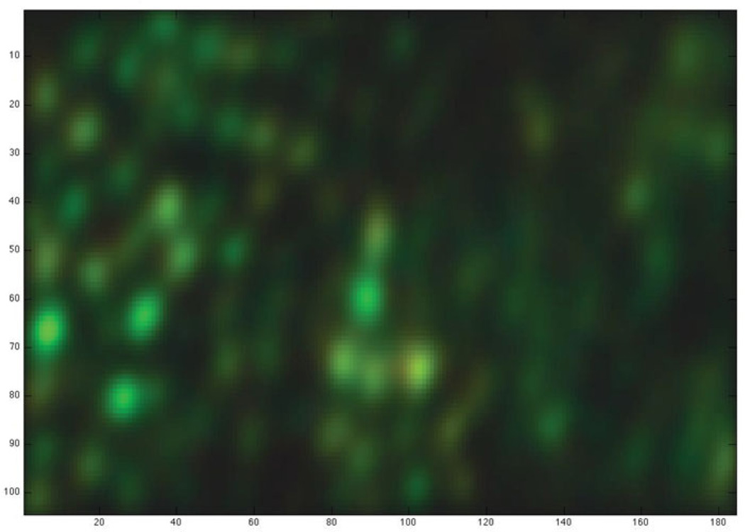
Consider the three cones which could possibly be placed at a particular location, represented by the three column vectors w_red, w_green and w_blue. To visualize the evidence for placing a cone of each of the three colors at this location, we multiply the 3 × 1 vector of likelihoods [V (w_red) V (w_greengreen) V (w_blue)] by the 3-by-3 matrix COLOR^−l, where COLOR is the matrix of light sensitivities of the three cone types. This results in a RGB color vector where differences between the colors displayed for the evidence for the three types of cones are more pronounced; it is most particularly useful to exaggerate color differences because the spectral sensitivity of red and green cones are so close that the difference between evidence for these two cone types would not otherwise be distinguishable in the plot. Figure 1) shows the resulting evidence map for the first dataset we will examine below.

Figure 1.

Visual summary of the evidence for cones across spatial locations. Dark areas show less evidence for the presence of a cone, while red, green and blue areas show evidence for cones of the corresponding types. The colors displayed, which cannot be assigned meaningful units, were obtained as explained in the main text. The axes count the number of possible cone positions considered, which is 4 times the number of pixels in the stimulus: the evidence map is supersampled by a factor of 4 compared to the original stimulus and STAs.

MCMC sampling

Using our likelihood (7), our goal is to infer likely cone configurations, consisting of a set of cone locations and colors. Because of the hard cone exclusion prior, the space of possible cone configurations is not a simple subset of a vector space, complicating inference. In this context, one method for finding likely configurations could involve sampling from the posterior distribution using Markov Chain Monte Carlo (MCMC) methods (Robert and Casella 2005). An MCMC chain is a random walk in the space of admissible cone configurations, where care has been taken to ensure that the time spent visiting a configuration is proportional to its posterior probability, at least asymptotically. Starting from an initial configuration which may not be very likely, the configuration will walk randomly towards more likely configurations, during an initial phase called burn-in, where the chain is not yet stationary in its distribution of sampled configurations. The MCMC chain will eventually reach the region of likely configurations, where it will spend most of its time, sampling in a stationary manner from the posterior distribution.

In order to ensure that the stationary distribution of the random walk coincides with our desired posterior p(cones|data), it is sufficient that the transition probabilities t(cones′ | cones) governing the walk satisfy detailed balance:

$$t(\mathit{\text{cones}}\prime |\mathit{\text{cones}})𝓅(\mathit{\text{cones}}|\mathit{\text{data}})-t(\mathit{\text{cones}}|\mathit{\text{cones}}\prime )𝓅(\mathit{\text{cones}}\prime |\mathit{\text{data}}).$$

We ensure that our random walk t(cones′|cones) satisfies detailed balance by using the Metropolis-Hastings algorithm (Robert and Casella 2005). From configuration cones, a move to a candidate configuration cones′ is proposed randomly with probability proposal(cones′ | cones), and with a probability proposal(cones| cones′) of proposing the reverse move from cones′. We then accept the proposed move with probability

$${𝓅}_{\mathit{\text{accept}}}(\mathit{\text{cones}}\prime |\mathit{\text{cones}})=\text{min}(1,\frac{𝓅(\mathit{\text{cones}}\prime |\mathit{\text{data}})\mathit{\text{proposal}}(\mathit{\text{cones}}|\mathit{\text{cones}}\prime )}{𝓅(\mathit{\text{cones}}|\mathit{\text{data}})\mathit{\text{proposal}}(\mathit{\text{cones}}\prime |\mathit{\text{cones}})}).$$ (8)

.

Finding the set of likely cone configurations entails sampling from the product of the likelihood (the exponential of (7)) with the hard cone exclusion prior on cone configurations. We sample from this distribution with a random walk in the allowed cone configuration space. However, because of the hard exclusion prior, the posterior has many deep local optima, and naive MCMC samplers will get stuck in these traps, leading to unacceptably slow mixing.

The sampling problem behaves differently in regions of visual space where the ganglion cell recordings carry strong evidence about cone locations, and regions with a dearth of evidence. A region with strong evidence, for example at the location of an STA from a ganglion cell with many spikes, will constrain cone placement more than a region outside of the receptive field center of all recorded ganglion cells. In Figure 1, the former show as bright regions, while the latter are dark.

For regions where there is a lot of evidence for cones, the typical differences in likelihood between different configurations are very large: if we were to sample from the distribution of cone configurations in such regions, one particular configuration could prevail as being astro- nomically more likely than all other configurations. For these regions, all that is important is to find the single most likely configuration. On the other hand, in regions where there is little evidence constraining cone configurations, the small differences in likelihoods of various configurations warrant sampling from the ensemble of possible configurations.

In order for MCMC to sample the set of likely cone configurations without getting stuck in deep wells of probability arising from regions with strong evidence and the cone exclusion prior, we combine two strategies: we take care to only propose Monte Carlo moves which respect the cone exclusion prior, and we use an adaptive simulated tempering technique (Salakhutdinov 2010) which effectively flattens the likelihood landscape, keeping the sampler from getting stuck in local maxima of likelihood.

Adaptive simulated tempering

In order to avoid getting stuck in local maxima, we use the CAST (Coupled Adaptive Simulated Tempering) sampler proposed in (Salakhutdinov 2010). This sampler is a hybrid (Atchade and Liu 2010) of the Wang-Landau algorithm (Wang and Landau 2001) and of the sampling scheme known as simulated tempering (Marinari and Parisi 1992), closely related to parallel tempering, aka replica exchange Monte Carlo, all of which flatten the likelihood landscape using an additional parameter γ which plays the role of an inverse temperature in physics; see (Earl and Deem 2005) for a review. The common idea in all these schemes is to replace the data likelihood p(data |cones) with a family of functions p_γ(data |cones) where p_γ=1 (data | cones) is equal to p(data | cones), and which become flatter (with less pronounced local maxima) as γ moves away from 1. We are only interested in samples from the true distribution, i.e. p_γ=1, but we also let the system reach other values of γ at which it can escape from local maxima. See the next section for our particular definition of p_γ.

The CAST sampler consists of two MCMC chains that run in parallel, a so-called “fast” chain and a “slow” chain. The slow chain has fixed γ = 1, so it samples the desired distribution of cone configurations using the Monte Carlo moves detailed above. Because it has γ = 1, the slow chain often gets stuck in local maxima on its own. The fast chain has a γ which is allowed to fluctuate among a predefined ordered set of values after every regular Monte Carlo move. The set of γ ranges from 1 to values far enough from 1 to ensure that local maxima are shallow and do not trap the chain. The fluctuations of γ are controlled by a Wang-Landau scheme (Wang and Landau 2001; Atchadé and Liu 2010), which by design ensures that γ samples the whole range of available values roughly uniformly. In particular, the γ variable is guaranteed to regularly visit both values far from 1, where local maxima are not a problem, and the value γ = 1 we are interested in. We used 20 values of γ, ranging from 1 to values which flatten the likelihood enough to ensure that the fast chain does not get stuck in local minima (see section below on flattening the likelihood). The 20 steps between the hottest temperatures and temperature 1 allow the fast chain to cool down to configurations that are more typical of the slow chain as it reaches temperature 1. Since the Wang-Landau scheme ensures that the fast chain samples all temperatures, the exact progression of temperatures used is less important than for other schemes such as parallel tempering, for which the temperature schedule must be chosen very carefully (Earl and Deem 2005).

Whenever the fast chain returns to γ = 1, we allow for cones to be swapped between the slow and fast chains' cone configurations. However, we do not swap the whole cone configurations between the two chains, as the simulated tempering algorithm usually entails; instead, we choose the smallest possible subsets of cones to be swapped, so as to maximize the probability of accepting swap moves, ensuring that information is transferred as fluidly as possible between the two chains (see the end of this section for how these subsets of cones are chosen). This exchange of cones between the slow and fast configurations will often knock the slow chain’s cone configuration out of a local maximum it was stuck in. Swapping a particular subset of cones in the fast chain with a subset of cones in the slow chain is accepted or rejected according to how the swap affects the joint log-likelihood log p_fast(data | cones_fast) + log p(data | cones_slow) using the Metropolis-Hastings acceptance probability (8) as for regular MCMC moves, where p_fast is the distribution sampled from by the fast chain when γ = 1.

The groups of cones proposed for swapping are chosen to be the smallest groups that can be swapped with each other without violating the cone exclusion distance. These groups of cones can be found by simple agglutination. If cone₁ in the fast chain overlaps cone₂ in the slow chain, then these two cones must be swapped together. If in turn cone cone₂ in the slow chain overlaps cone cone₃ in the fast chain, all three cones must be swapped together. This agglutination is continued until the cones in the group overlap no other cones than themselves. If cones are left that have not been agglutinated into a group yet, a new group is started with one of them chosen at random. This agglutination could in principle “percolate,” leading to minimal groups of cones which comprise most or all of the cones across the two chain configurations. However, in practice, the sizes of groups obtained via this procedure are small and localized. This is very convenient, since the smaller the groups of cones proposed for swapping, the greater the chances of accepting that MCMC move.

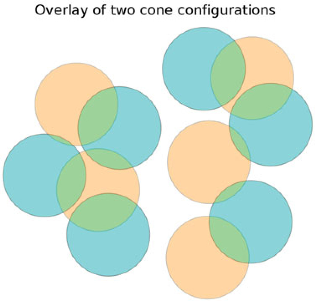
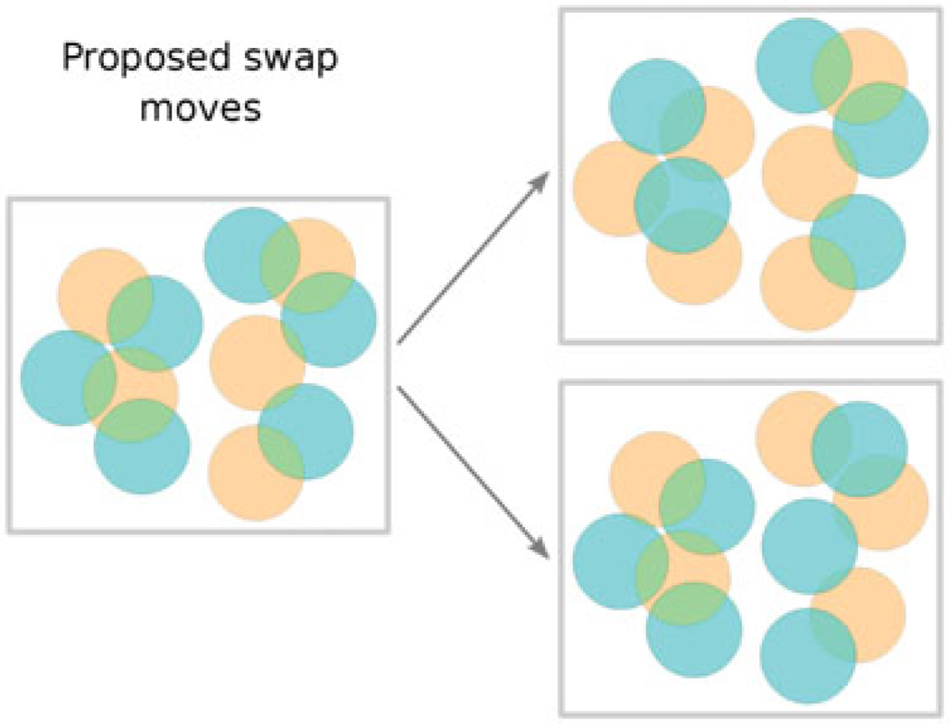
More formally, the agglutination procedure described above is a simple algorithm for computing the transitive closure (Lidl and Pilz 1997) of the overlap relation ℛ between cones. For cone₁ in the fast chain and cone₂ in the slow chain, ℛ(cone₁, cone₂) is true if and only if swapping cone₁ out of the fast chain would require swapping cone₂ out of the slow chain in order to preserve cone exclusion. In other words, ℛ(cone₁, cone₂) is true when the two cones overlap in space, even though they currently belong to different chains. This relation ℛ is reflexive (every cone overlaps itself) and symmetric (if cone₁ overlaps cone₂, then cone₂ overlaps cone₁). The ‘must be swapped together’ relation ℬ which we calculate is the transitive closure of ℛ: it is the smallest binary relation which is implied by ℛ and which is also transitive, i.e. for which ℬ(cone₁, cone₂) and ℬ(cone₂, cone₃) implies ℬ(cone₁, cone₃). Calculating the transitive closure of ℛ is computationally straightforward: one proceeds by agglutination similarly to the way described above; we use a particularly simple and fast algorithm called the Floyd-Warshall algorithm (Roy 1959); Warshall 1962). Once it is obtained, this transitive closure defines a number of equivalence classes, i.e. a number of groups of cones which must be swapped together. Figure 2 shows an example in which two groups of cones must be swapped together, while Figure 3 shows the two corresponding swap moves.

Figure 2.

Overlay of the slow cone configuration (brown) and the fast cone configuration (cyan) in a toy example making the overlap relation apparent by partial transparency. Color here denotes belonging to one of the two chains, and is not to be confused with cone type, which is not denoted in this figure. In this toy example, the transitive closure of the overlap relation defines two equivalence classes of connected cones: one with five cones on the left, and one with six cones on the right. The equivalence class (or connected component) on the left has two brown and three cyan cones, while the one on the right has three brown and three cyan cones.

Figure 3.

For the same pair of configurations as in the previous figure (left), two swap moves would be considered, one for each equivalence class (right). Each of the two admissible swap moves consists in swapping the brown cones in one equivalence class with the cyan cones in the same equivalence class. Note that only the memberships in one of the two chain configurations are changed; cone type (not denoted in this figure) and spatial location are unchanged.

Our agglutination process for finding groups of cones to swap together is designed to find the smallest groups of cones that can possibly be swapped together without violating the cone exclusion distance. One notable property of the groups of cones we obtain is that if any of the groups of cones that form an equivalence class are swapped, the groups that would be found by agglutination for the new configurations are the same as the groups found before the swap. We use this property to calculate groups once, and then run several swap moves without needing to re-agglutinate groups. Any time the fast chain returns to γ = 1, we choose at most 50 such groups at random by Floyd-Warshall agglutination, and let Metropolis-Hastings accept or reject swaps using a group chosen among these at random 50 times. The likelihood used to accept or reject swap moves is the independent joint log-likelihood log 𝓅_fast(data | cones_fast) + log 𝓅(data |cones_slow), which as argued above ensures that the stationary distribution sampled by cones_slow is the desired distribution 𝓅(cones_slow | data).

Flattening the data likelihood

The most common method for “flattening” an energy landscape for simulated or parallel tempering is to simply scale the log-likelihood by a proportionality factor β, which is interpreted as an inverse temperature. In practice for our problem, this can help unfreeze cones that are in regions with very little evidence, while cones remain stuck in regions with mildly more evidence. We can try to unfreeze cones more uniformly across space by scaling the log-likelihood in a way that evens out the effective evidence. We do this by raising the ${\mathbf{\text{STA}}}_i^T\mathbf{W}\left({\mathbf{W}}^T\mathbf{W}\right)-1{\mathbf{W}}^T{\mathbf{\text{STA}}}_i$ term in (7) to a power δ smaller than 1. In this way, we carry out simulated tempering with a chain of data likelihoods of the form:

$$\text{log}𝓅(\mathit{\text{data}}|\mathit{\text{cones}},\beta ,\delta )=\sum _i\frac{N_{{\mathit{\text{spikes}}}_i}^2}{2\beta (N_{{\mathit{spikes}}_i}{\sigma }^2+g_i)}{({\mathbf{\text{STA}}}_I^T\mathbf{W}{({\mathbf{W}}^T\mathbf{W})}^{-1}{\mathbf{W}}^T{\mathbf{\text{STA}}}_i)}^{\delta }+\sum _i\frac{\mathit{\text{dim}}({\mathbf{a}}_i)}{2\beta }\text{log}(\frac{g_i}{N_{\mathit{\text{spikes}}}{\sigma }^2+g_i})$$ (9)

.

In practice, we allow the temperature to take 20 values γ = (β, δ) ranging from (1,1) to (0.2, 0.1).

Monte Carlo moves

The data likelihood (9) depends only on the set of cone locations and colors, since the weights from cones to ganglion cells have been marginalized out. The posterior we wish to sample from consists of the product of the data likelihood with the hard cone exclusion prior. Sampling proceeds by only proposing random changes in the current cone configuration that respect the hard cone exclusion prior, accepting or rejecting each change in accordance to the data likelihood.

The proposed Monte Carlo moves we use are generated as follows: first, a possible cone location is chosen. With 50% probability, a location which is currently unoccupied by a cone and which is far enough from existing cones to avoid cone exclusion is chosen; one of the three cone types is chosen to be added to that location. With 50% probability, a location which is already occupied by a cone is chosen; for the cone already present at that a location, the possible moves are to change its color, remove it, or shift it to a neighboring pixel. For the chosen move, forward and backward proposal probabilities are calculated, and the move is then accepted or rejected using the Metropolis-Hastings acceptance probability (8).

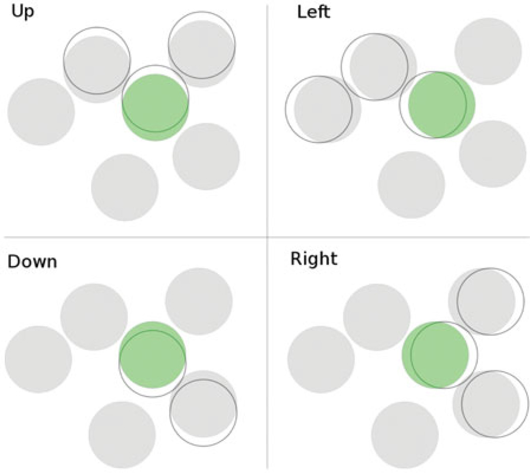
During moves which consist in shifting an existing cone to a neighboring location, shifts are propagated to any cones that are in the way: for example, the naive move consisting in shifting a single cone to the left is replaced by a shift to the left of all cones which must be moved together in order to respect the cone exclusion (Figure 4). In other words, if there are one or more cones in contact with the left of the cone being shifted, those cones are bumped over to the left with it. Any cones which are bumped off of the region of possible cone locations considered are deleted.

Figure 4.

Shift moves in the four cardinal directions. The modified cone locations in each proposed move are denoted by empty circles. Shifting the green cone in each direction induces shifts of cones that are in the way.

Results

Datasets

We apply our cone finding algorithms to two datasets, one collected from 21 ganglion cells, and one collected from 324 ganglion cells. Our model only requires knowing these cells' STAs, the number of recorded spikes for each cell, and the mean and variance of the stimulus at each pixel. For the first dataset, we limit ourselves to a region of interest in cone location space which spans 26 by 46 stimulus pixels (see (Field et al. 2010) for full details, scale bars, etc.); for the second dataset, we limit ourselves to an area of 160 by 160 pixels. These regions were chosen to include most of the power from all the ganglion cell STAs. As mentioned earlier, permissible cone locations were chosen to be a square lattice 4 times finer than the pixel lattice, for a total of 16 possible cone locations per pixel.

Apart from their difference in size, the main difference between the two datasets is that the first one has positive evidence in almost all locations, whereas the second larger dataset has many areas where the evidence is not strong enough to warrant placing cones with any confidence.

The greedy algorithm

We compare our MCMC results to the configuration obtained by a straightforward greedy procedure: using the same posterior log-likelihood (7) as the MCMC algorithm, cones are added one by one with the location and type that maximizes the posterior given all the cones accumulated so far. This greedy accumulation of cones starts without cones, and stops when adding a cone can only reduce the posterior. See Figures 5–8.

Figure 5.

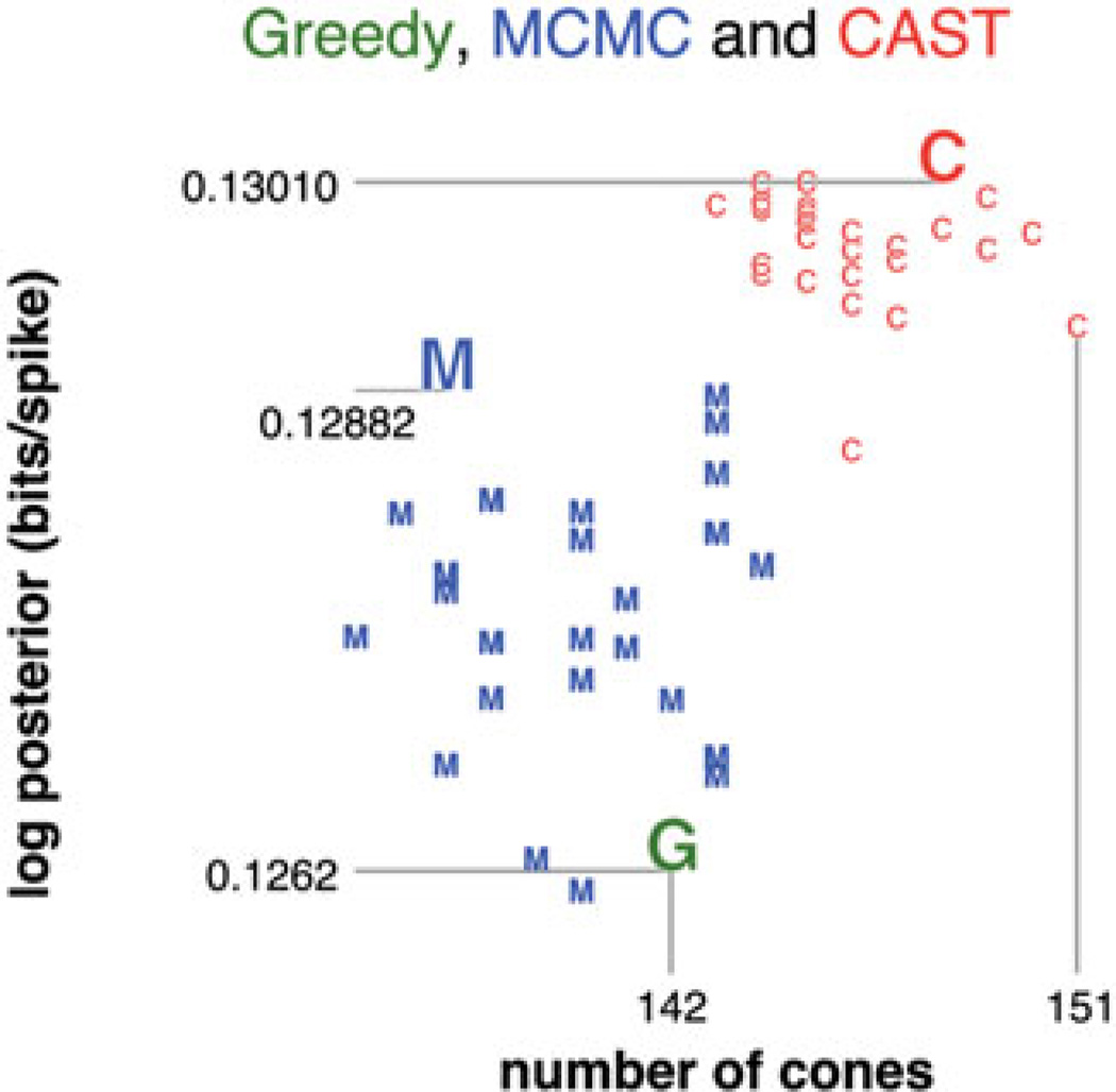
First dataset: posterior log-likelihood plotted against number of cones for (G) the greedy solution, (M) the best configurations over 30 simple MCMC runs with 10⁶ iterations, and (C) the best configurations over 30 CAST runs with 10⁶ iterations. MCMC configurations were reinitialized to the lazy greedy cone configuration (see the MCMC and CAST results section) whenever the likelihood did not improve for 400 consecutive iterations. In each category (G, M and C), the marker for the cone configuration with highest likelihood is magnified, and its log-posterior likelihood given. All log-likelihoods are in bits per spike.

Figure 8.

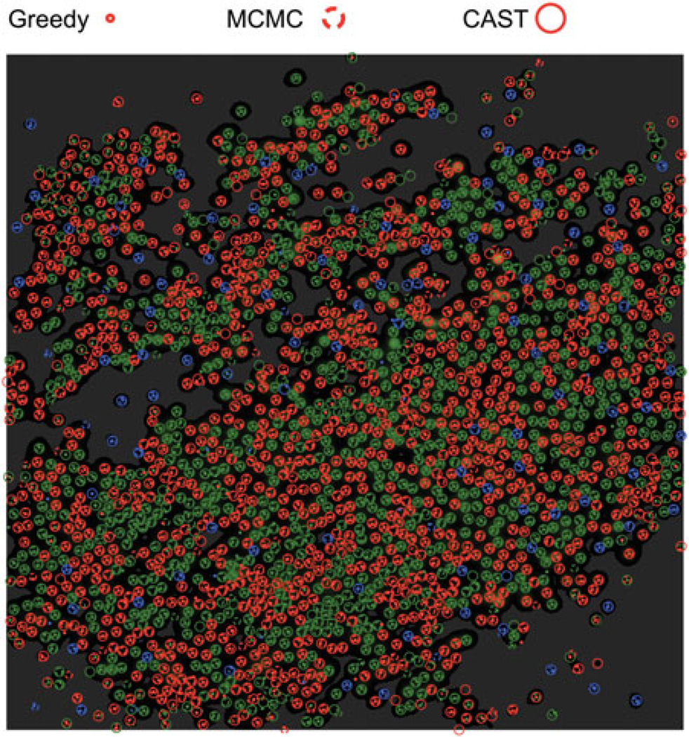
Second dataset: superposition of the greedy configuration with the best CAST and MCMC configurations, as in Figure 7. Cones concentrate mostly in bright regions, i.e. in regions with a lot of evidence for cones of a particular color. Regions that are darker than a certain threshold are devoid of cones, because the evidence for cones in these regions is smaller than the penalty incurred for adding a new cone, which is induced by the prior on weights (see text explaining eq. (7)); such regions have been uniformly colored a lighter shade of grey.

The greedy algorithm, while quick to find configurations with many cones and reasonably high likelihoods, has several drawbacks. One drawback is that by committing to each cone’s placement greedily, we are missing opportunities to increase the likelihood by shifting groups of cones which are in contact together. This can be seen by seeding an MCMC run with the result of the greedy algorithm: the likelihood increases quickly from the first few MCMC iterations as groups of nearby cones shift by small distances, relaxing into more likely positions.

Another less obvious drawback of the greedy algorithm is that it is difficult to estimate the number of cones whose inference we can be confident about. This problem can be seen by tracking the increase in likelihood as a function of the number of cones (Figure 9). With the greedy algorithm, the likelihood plateaus many iterations before the algorithm terminates (that is, when the addition of any further cones would decrease the posterior): the last cones added only contribute very little to the likelihood. This is most notable on our second dataset, which has both areas with high evidence and areas with zero to little evidence; for this dataset, the log-likelihood increases from 0.0548 bits/spike for 1689 cones to 0.0549 bits/spike for 1879 cones. The greedy algorithm places as many cones as can fit in the areas with non-zero evidence, however small this evidence, without giving any indication as to how confident we can be in each cone’s position or color. This makes it very difficult to say with confidence how many cones should be kept, and which cones should be considered to be spurious or poorly constrained by the observed data.

Figure 9.

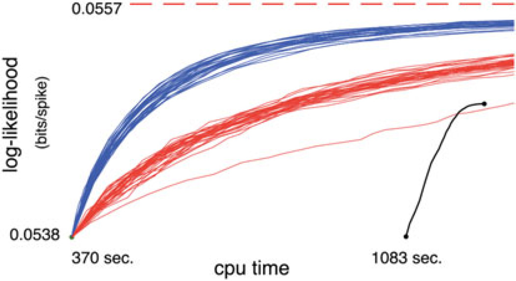
The log-likelihoods attained by the greedy (black), MCMC (blue), and CAST (red) methods are plotted against CPU run time, for the second, larger dataset. All times and likelihoods smaller than those obtained from the lazy greedy algorithm (green dot) are not shown; in particular, the first 1083 seconds of the greedy algorithm, during which the greedy configuration had a smaller likelihood than the lazy greedy configuration, are not shown. All the MCMC and CAST runs were initialized with the lazy greedy configuration: each run starts at the same green dot. The thick dotted red line indicates the best likelihood eventually obtained from the best of 30 CAST runs, after 36 hours.

Note that all of the results shown here and below are evaluated on the full data set, with no splitting between “training” and “test” data, because our focus is on how well the algorithms are able to explore and optimize the full log-posterior, rather than the predictive error of the resulting estimators.

MCMC and CAST results

We ran 30 MCMC and CAST chains for both datasets for 10⁶ iterations each. Each chain was initialized with the same configuration obtained by a faster version of the greedy algorithm, which we will call the “lazy” greedy algorithm, and which we now briefly describe. (An advantage of the methods described here is that they are highly parallelizable. All analyses performed here were performed on a parallel cluster computer; similar analyses performed in serial on a single processor would be feasible, but slower by an order of magnitude.)

Implementing the greedy algorithm requires keeping a map of how much the likelihood would increase if a cone were to be added at each possible available location and color. This map allows us to select the single cone addition which will increase the likelihood the most. Every time a new cone is added, this map of likelihood increases must be updated within the vicinity of the new cone. It is easy to devise a much faster but less precise algorithm which does not update the likelihood map after each cone addition. This leads to configurations which are of relatively poor quality, but are very fast to obtain, and which are reasonable enough to be used as the initial configuration for all of our MCMC and CAST chains.

Running naive MCMC leads to configurations with posterior likelihoods that stop increasing after a few thousand iterations: each MCMC run gets stuck in a small region of configuration space. Whenever an MCMC run likelihood did not increase for more than 400 (resp. 8500) consecutive iterations for the first (resp. second) dataset, it was reinitialized to the lazy greedy configuration. Even though naive MCMC runs get stuck in local optima, most of the resulting configurations have higher posterior likelihoods than the greedy configuration (Figures 5, 6 and 9). This is not surprising, since MCMC is similar to a greedy algorithm with (probabilistic) backtracking.

Figure 6.

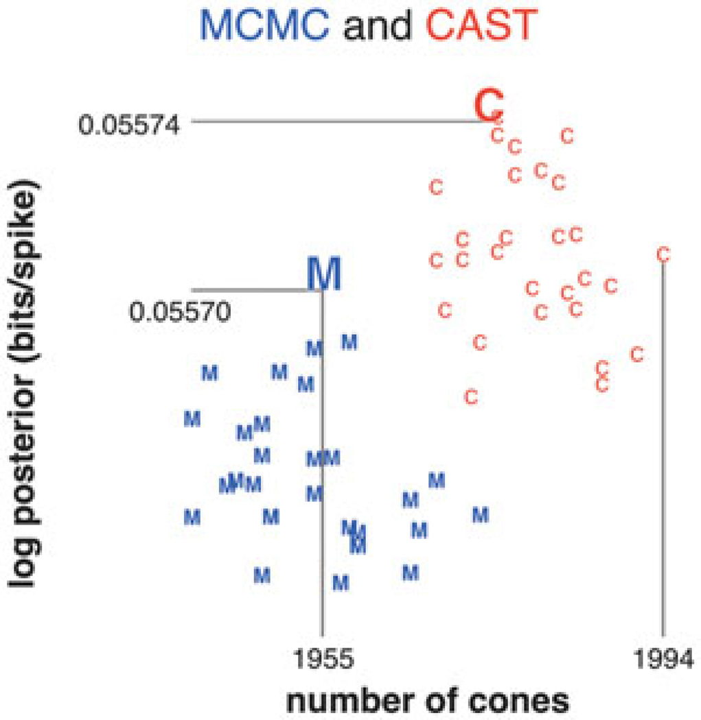
Second dataset: posterior log-likelihood plotted against number of cones. Conventions as in Figure 5, except MCMC configurations were reinitialized whenever the likelihood did not improve for 8500 consecutive iterations. For comparison, the log-likelihood per spike for the greedy solution was significantly lower, with 0.0549 bits per spike for 1879 cones.

Running 30 instances of CAST for 10⁶ iterations each, we see that CAST consistently explores regions of cone configuration space with more cones and higher likelihoods than either the greedy or naive MCMC methods (Figures 5 and 6). CAST runs did not need to be reinitialized, as the likelihoods involved typically increase throughout the 10⁶ iterations. However, it is hard to say whether or not these chains are ergodic. All chains do not attain the same range of log-likelihoods by the end of their run; this could either be due to the chains not being ergodic, or to 10⁶ not being a long enough “burn-in” period for the chain to reach the regime of typical configurations.

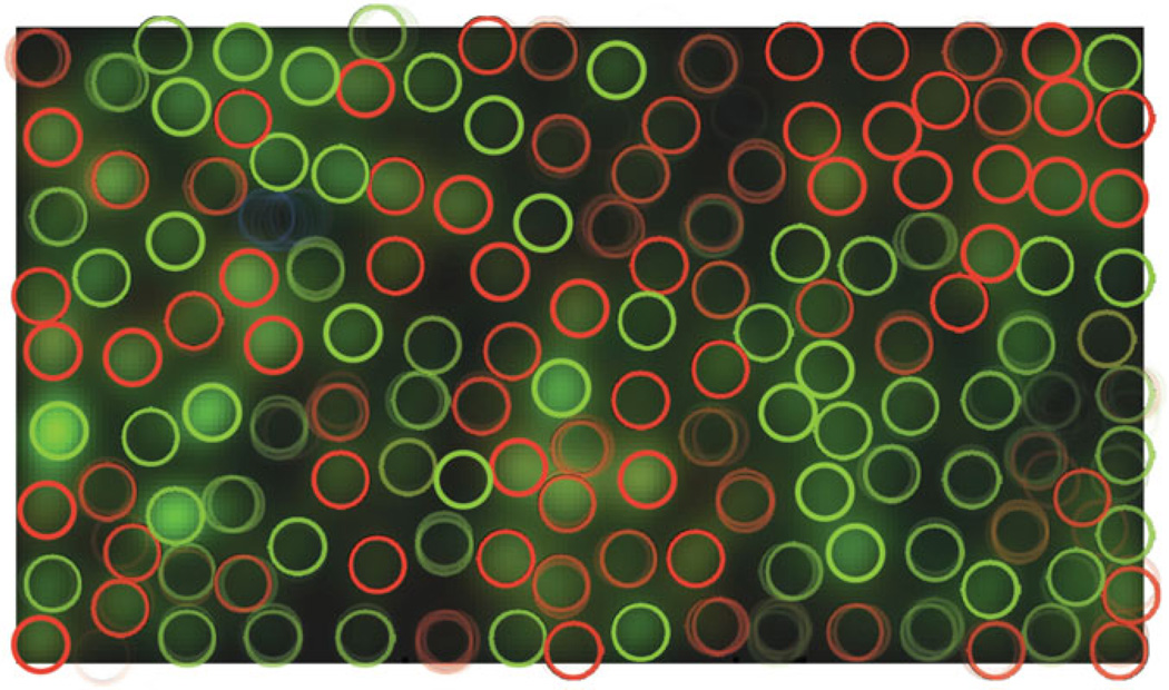
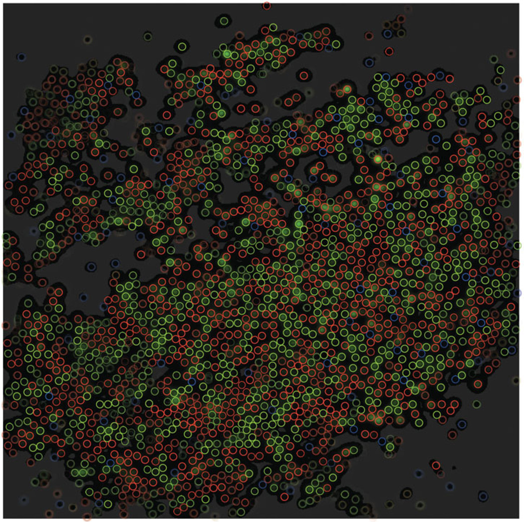
CAST runs offer a good indication of how confident we can be in each cone inference, since they are sampling from a distribution of likely cone configurations while being less prone to local optima. We can for example plot cone configurations averaged over many CAST iterations (Figures 10 and 11). In these plots, cones have a color which is an average of the colors of cones found at a same location across samples, and an opacity which is proportional to the number of samples for which a cone was present at that location. Cones whose inferences are uncertain are either faded out by partial transparency, have a color which is a mix of green and red, or a position which is uncertain, depending on the type of uncertainty. The proportion of samples for which a cone is present at a given location gives an easily interpretable indication of how certain we are of the cone’s inference.

Figure 10.

Ensemble of cone configurations as sampled by the best CAST chain out of 30 for the first dataset. Each depicted cone has a transparency reflecting the proportion of sample configurations where a cone was present at its location, and a color which is an average of the colors of all the cones that were placed in this location. This plot allows us to visualize the degree of confidence we can have in each cone inference.

Figure 11.

Ensemble of cone configurations as sampled by the best CAST chain out of 30 for the second dataset. Conventions as in Figure 10.

Application: denoising receptive field estimates

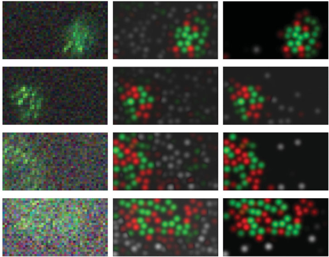
As a simple application of the methods discussed above, we consider a basic problem: how do we construct efficient estimators of the receptive fields k_i? In particular, can we exploit the fact that we are observing multiple ganglion cells simultaneously, to obtain better estimates than would be possible in the “classical” setting, where only one ganglion cell is observed per experiment? In the latter case, the standard approach (as discussed above) is to use the STA as an estimator for k (Chichilnisky 2001); Paninski 2004). However, in these experiments STAs are highly noisy, due to the low effective contrast and the fine pixelization of the stimulus; see the left panels of Figure 12 for some examples, and (Paninski 2003) for further discussion of the variability of STA-based estimates.

Figure 12.

Denoised estimates of individual ganglion cell receptive fields. Left panels: raw STAs of four simultaneously recorded genglion cells, taken from dataset 1. Middle: posterior mean receptive fields 𝔼(W_ai | data), for each of the four cells. Colors correspond to positively-weighted cones (with higher intensity corresponding to larger inferred weights a); grayscale corresponds to magnitude of negatively-weighted cones (i.e., the inhibitory surround). Right: thresholded estimate of the receptive fields (see text for details). Top two rows are midget cells; bottom two rows are parasol cells.

Of course, a natural alternate approach here is to exploit the fact that all of the observed ganglion cells share a common set of cones whose configuration we have estimated. We have already discussed above how to compute the conditional expectation 𝔼 (a_i | data) of the receptive field weights, given the output of our MCMC samplers; now we need simply multiply these weight vectors by the corresponding cone-to-pixel matrix W to obtain estimates of the receptive fields. See the middle panels of Figure 12 for an illustration.

In fact, we can go further: since we also have access to the posterior uncertainty about the weights a (through Cov (a_i | data), we can threshold any elements of the weight vector about which we have insufficient posterior confidence, to further denoise the estimate. In the right panels of Figure 12, we discarded any element of a for which the conditional expectation was less than two standard deviations away from zero. (Of course other approaches are possible here.) These results therefore illustrate the power both of simultaneous recording and also hierarchical modeling: by “sharing information” between simultaneously recorded ganglion cells (via our estimate of the cone layer), we obtain significantly sharper estimates of the ganglion cell parameters than would have been possible otherwise.

Conclusion: using the greedy, MCMC, and CAST algorithms

Our analyses consistently demonstrate that MCMC (and particularly CAST) methods achievehigher likelihood scores than does the greedy algorithm. Of course, in practice, it may be useful to use a suboptimal algorithm if it is significantly faster, and in particular if it leads to reasonable cone configurations fast enough for online use during an experiment.

Thus it is useful to conclude by taking another look at the typical running times of the various methods on current hardware for our larger dataset, which has a size typical of most experiments (Figure 9). The “lazy” greedy configuration used to initialize the MCMC and CAST runs gives them a significant head start over the greedy method. The MCMC likelihoods quickly exceed the final greedy configuration’s likelihood. In the process, the MCMC method quickly corrects mistakes made by the lazy greedy algorithm’s crude approximation, adding cones which were missed by the lazy greedy method. This makes initializing our naive MCMC runs with the lazy greedy configuration the method of choice for fast evaluation of the cone configuration during an experiment.

By comparison, the CAST method takes much longer to increase likelihoods. However, it does not get stuck in local optima as the naive MCMC method does, and CAST configurations end up with significantly higher likelihoods than all other methods (Figures 5 and 6). Thus a reasonable approach is to initialize with the fast lazy greedy method, then relax into a local optimal solution with MCMC, and finally to continue with CAST for as many iterations as desired to evaluate the true posterior over cone configurations for a given experiment.

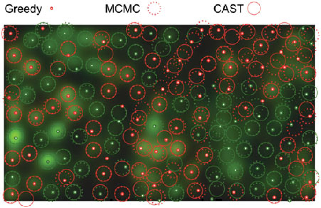
Figure 7.

First dataset: superposition of the greedy configuration, the most likely configuration out of 3 × 10⁶ iterations worth of MCMC runs, and the most likely out of as many iterations of CAST runs. The background color-scale image is a depiction of the evidence for the presence of cones of different colors across visual space (see main text).

Appendix/Supplemental

STA space-time separation using SVD

In a preprocessing step, the STA of each ganglion cell was approximated as being separable in space and time. (Small deviations from separability — specifically, center-surround latency differences — are present in these cells' receptive fields; see (Chichilnisky and Kalmar 2002) for further details. However, the stimulus refresh in these experiments is sufficiently slow that these small inseparabilities are negligible here.) The temporal and spatial components were obtained using a singular value decomposition (SVD) approach, as in (Gauthier et al. 2009). First, the STA was put in a matrix M in which each row was the time course of a single pixel. The SVD consisted of decomposing M = UDV^T, where U and V are orthogonal matrices and D is diagonal with positive decreasing elements along the diagonal. The STA matrix M was approximated as being separable in space and time by setting all but the first element in D to zero, revealing the first column of U as the STA spatial component, and the first row of V as the STA temporal component. Finally, the spatial stimulus s_t discussed in the main text is defined as the projection of the full spatiotemporal stimulus onto the SVD-derived temporal component.

Some implementation details

In the actual implementation, W is never represented explicitly. This is because many of the calculations required for the MCMC simulation can be done in advance: the matrix W always appears in calculations either multiplied on the left by STA, or on the left by its own transpose. Since STAs are limited in space, their dot product with the cone receptive fields in W is sparse. The sparsity structure of these dot products is calculated in advance for all possible cone locations. The actual dot products are then only calculated for combinations of cone locations and STAs which are known to have a significant dot product (see main text for details).

We also exploit the sparsity of W^T W: this matrix contains dot products between pixelized cone receptive fields, which are non-zero only for overlapping cones. In addition, these dot products only depend on the relative differences in the positions of the two cones. We take advantage of this by only considering a finite number of possible cone locations that are regularly spaced with a frequency which is a multiple of the stimulus pixel width. With such regular spacing, the relative distances between overlapping cones can only take a few values, so the values populating W^T W can be calculated in advance. Currently, there are 4 cone coordinate locations for each pixel width, for a total of 16 possible cone locations per pixel. This allows us to calculate in advance the 16 pixelated convolutions of the typical cone receptive field spatial component with itself, where the pixelation consists of integrating over the square surface of each pixel as explained in the main text.

Another implementation detail which is important for speed is to keep track of which cones are touching which others in the four cardinal directions. Indeed, whenever a cone shift move is proposed, we need to know which neighboring cones to shift over with it in order to respect cone exclusion: it is more efficient to calculate the four neighborhood relations only once when an MCMC move is accepted rather than calculating them each time a new move is proposed, and these relations can be kept track of incrementally.

The code is available upon request.

References

- Atchade Y, Liu J. The wang-landau algorithm in general state spaces: Applications and convergence analysis. Statistica Sinica. 2010;20(1):209. [Google Scholar]
- Casella G, Berger R. Statistical Inference Pacific Grove. CA: Duxbury Press; 2001. [Google Scholar]
- Chichilnisky E. A simple white noise analysis of neuronal light responses. Network: Computation in Neural Systems. 2001;12:199–213. [PubMed] [Google Scholar]
- Chichilnisky E, Baylor D. Receptive-field microstructure of blue-yellow ganglion cells in primate retina. Nature Neuroscience. 1999;2:889–893. doi: 10.1038/13189. [DOI] [PubMed] [Google Scholar]
- Chichilnisky E, Kalmar R. Functional asymmetries in on and off ganglion cells of primate retina. J Neurosci. 2002;22(7):2737–2747. doi: 10.1523/JNEUROSCI.22-07-02737.2002. [DOI] [PMC free article] [PubMed] [Google Scholar]
- Diaconis P, Freedman D. Asymptotics of graphical projection pursuit. Annals of Statistics. 1984;12:793–815. [Google Scholar]
- Earl D, Deem M. Parallel tempering: Theory, applications, and new perspectives. Physical Chemistry Chemical Physics. 2005;7(23):3910–3916. doi: 10.1039/b509983h. [DOI] [PubMed] [Google Scholar]
- Field G, Gauthier J, Sher A, Greschner M, Machado T, Jepson L, Shlens J, Gunning D, Mathieson K, Dabrowski W, et al. Functional connectivity in the retina at the resolution of photoreceptors. Nature. 2010;467(7316):673–677. doi: 10.1038/nature09424. [DOI] [PMC free article] [PubMed] [Google Scholar]
- Frechette E, Sher A, Grivich M, Petrusca D, Litke A, Chichilnisky E. Fidelity of the ensemble code for visual motion in the primate retina. J Neurophysiol. 2005;94(1):119–135. doi: 10.1152/jn.01175.2004. [DOI] [PubMed] [Google Scholar]
- Gauthier JL, Field GD, Sher A, Greschner M, Shlens J, Litke AM, Chichilnisky EJ. Receptive fields in primate retina are coordinated to sample visual space more uniformly. PLoS Biol. 2009;7(4):e1000063. doi: 10.1371/journal.pbio.1000063. [DOI] [PMC free article] [PubMed] [Google Scholar]
- Keat J, Reinagel P, Reid R, Meister M. Predicting every spike: a model for the responses of visual neurons. Neuron. 2001;30:803–817. doi: 10.1016/s0896-6273(01)00322-1. [DOI] [PubMed] [Google Scholar]
- Lidl R, Pilz G. Applied Abstract Algebra. New York, NY: Springer; 1997. [Google Scholar]
- Litke A, Bezayiff N, Chichilnisky E, Cunningham W, Dabrowski W, Grillo A, Grivich M, Grybos P, Hottowy P, Kachiguine S, et al. What does the eye tell the brain?: Development of a system for the large scale recording of retinal output activity. IEEE Transactions on Nuclear Science. 2003;51(4):1434–1440. [Google Scholar]
- Marinari E, Parisi G. Simulated tempering: A new monte carlo scheme. EPL (Europhysics Letters) 1992;19:451. [Google Scholar]
- Paninski L. Convergence properties of some spike-triggered analysis techniques. Network: Computation in Neural Systems. 2003;14:437–464. [PubMed] [Google Scholar]
- Paninski L. Maximum likelihood estimation of cascade point-process neural encoding models. Network: Computation in Neural Systems. 2004;15:243–262. [PubMed] [Google Scholar]
- Paninski L, Pillow J, Simoncelli E. Maximum likelihood estimation of a stochastic integrate-and-fire neural model. Neural Computation. 2004;16:2533–2561. doi: 10.1162/0899766042321797. [DOI] [PubMed] [Google Scholar]
- Park I, Pillow J. Bayesian spike-triggered covariance analysis. Advances in Neural Information Processing Systems. 2011;24:1692–1700. [Google Scholar]
- Pillow J, Paninski L, Uzzell V, Simoncelli E, Chichilnisky E. Prediction and decoding of retinal ganglion cell responses with a probabilistic spiking model. Journal of Neuroscience. 2005;25:11003–11013. doi: 10.1523/JNEUROSCI.3305-05.2005. [DOI] [PMC free article] [PubMed] [Google Scholar]
- Pillow JW, Shlens J, Paninski L, Sher A, Litke AM, Chichilnisky EJ, Simoncelli EP. Spatio-temporal correlations and visual signalling in a complete neuronal population. Nature. 2008;454(7207):995–999. doi: 10.1038/nature07140. [DOI] [PMC free article] [PubMed] [Google Scholar]
- Ramirez A, Paninski L. Fast inference in generalized linear models via expected log-likelihoods. Under review. 2012 doi: 10.1007/s10827-013-0466-4. [DOI] [PMC free article] [PubMed] [Google Scholar]
- Robert C, Casella G. Monte Carlo Statistical Methods. New York, NY: Springer; 2005. [Google Scholar]
- Roy B. Transitivité et connexité. C. R. Acad. Sci. Paris. 1959;249:216–218. [Google Scholar]
- Salakhutdinov R. Learning deep Boltzmann machines using adaptive MCMC. In Proceedings of the International Conference on Machine Learning; 2010. [Google Scholar]
- Segev R, Goodhouse J, Puchalla J, Berry M. Recording spikes from a large fraction of the ganglion cells in a retinal patch. Nature Neuroscience. 2004;7:1154–1161. doi: 10.1038/nn1323. [DOI] [PubMed] [Google Scholar]
- Wang F, Landau D. Efficient, multiple-range random walk algorithm to calculate the density of states. Physical Review Letters. 2001;86(10):2050–2053. doi: 10.1103/PhysRevLett.86.2050. [DOI] [PubMed] [Google Scholar]
- Warshall S. A Theorem on Boolean Matrices. J. ACM. 1962;9:11–12. [Google Scholar]