

Abstract
Genome projects now produce draft assemblies within weeks thanks to advanced high-throughput sequencing technologies. For milestone projects like E. coli or H. sapiens, teams of scientists were employed to manually curate and finish these genomes to a high standard. Nowadays, this is not feasible for most projects and the quality of genomes is generally of a much lower standard. This protocol describes software (PAGIT, post-assembly genome-improvement toolkit) to improve the quality of draft genomes. It offers flexible functionality to close gaps in scaffolds, correct base errors in the consensus sequence, and to exploit reference genomes (if available) for improving scaffolding and generating annotations. The protocol is most accessible for bacterial and small Eukaryotic genomes (up to 300 Mb), such as pathogenic bacteria, malaria and parasitic worms. Applying PAGIT to an E. coli assembly takes approximately 24 hours: it doubles the average contig size and annotates over 4300 gene models.
Keywords: Next generation sequencing, automatic finishing, gap closing, genome annotation, contig ordering
Introduction
The ultimate goal of many genome projects is to generate a gap-free and fully annotated genome. Next Generation Sequencing (NGS) technology has greatly increased the through-put of DNA sequencing and as a result the number of draft genomes deposited in public databases has increased dramatically. However, although the quantity has increased, the quality of available genomes has suffered. This is because it is essential to engage in a very time-consuming process of manual editing and gap closure before a genome can be considered to be a finished or gold-standard product 1. For the human genome project the aspiration was to have a 1 bp error per 10 kb of finished sequence 2. In addition to generating accurate genome sequences, genome annotation is an important and time-consuming aspect of de novo genome sequencing projects. These projects aim to generate high quality annotated genomes that may be subsequently used as reference genomes – thus facilitating the re-sequencing and annotation of many related species through comparative methods 3, 4. For the vast majority of NGS genome projects the resources are simply not available to generate high-quality annotated sequences, and consequently many genomes may remain as poor quality drafts.
In genome projects, the sequencing reads generated by the NGS technologies are usually assembled using specialist software into large numbers of contigs (please see the glossary of terms in Box 1). Genome assembly is a very difficult computational problem and new approaches to assembly continue to be evaluated and developed5, 6. Gaps, or discontinuities, in the sequence invariably remain and are due to issues such as uneven sequence coverage, long repeats, segmental duplications, or technology biases. The resulting draft assemblies are thus frequently highly fragmented, incomplete and completely unannotated; regions of sequence within the draft will suffer from misassemblies, contamination, and low quality; and the error rate will be much higher than 1 bp per 10kb of assembled sequence. Furthermore, the types of error can be influenced by the characteristics of different sequencing technologies 7, 8. While draft genomes do contain useful information, they have significant limitations that may render complete and rigorous scientific analyses difficult or impossible1, 9.
BOX 1. Glossary of terms.
Alignment: the process of matching the order of bases between two or more DNA sequences so that the sequences map on to each other.
Annotation: identifying and ascribing functional descriptions to regions of the genome, including genes and coding sequences.
Genome assembly: the process of using reads to reconstruct the original genome from which they were derived.
Base calling: the automated process of determining the nucleotide base at a position in a sequence.
Base quality: a confidence score assigned to each base call. Low scores indicate a higher chance that the base may have been called incorrectly.
Consensus sequence: during genome assembly, when overlapping reads have been combined to form a contig with sufficiently high coverage, the most common base in the reads at each position is taken to be the consensus sequence.
Contig: a contiguous sequence of DNA assembled from overlapping reads.
Coverage: the number or depth of reads that cover (extend over) a section of DNA sequence.
De novo genome assembly: a genome assembly that is performed without referring to any existing genomes or reference sequences.
Draft genome assembly: a set of contigs and / or scaffolds generated by a computer program that attempts to reconstruct original chromosomal sequences from sequenced reads. Draft genomes are frequently highly fragmented, unannotated, and often contain assembly errors such as collapsed repeats.
Finished genome: the chromosomal sequences have been determined to an accuracy of at least 1 error in 10,000 base pairs. All contigs are placed in the right order and orientation along a chromosome with almost no gaps present. The sequence has been fully annotated.
Gaps: an unsequenced region of a scaffold that lies between two linked contigs.
Insert size: the average or expected number of (unsequenced) bases that lie between paired-end reads as measured from their outermost bases.
Indel: an insertion or deletion in a DNA sequence.
Mapping: aligning reads or other relatively short sequences to a longer sequence such as a finished genome.
N50: the length, for a set of different sized sequences, such that 50% of the genome is contained in sequences of at least that length. The larger the N50, the less fragmented the genome.
Paired-end reads or mate pairs: fragments of DNA sequenced from opposite ends of a larger fragment DNA that is of an approximately known size. Mate-pair libraries refer to large insert libraries sequenced over the paired-ends.
Read: data produced by a DNA sequencing machine from reading an individual DNA template in one direction.
Reference genome: a high quality draft or finished genome used to anchor alignments. The features of the sequence should have been annotated, and the contig length should be relatively long.
Scaffold or Supercontig: a portion of the genome sequence made by linking contigs together using paired-end reads. There will be gaps between the contigs comprising the scaffold.
Synteny: the conserved gene order that is observed along the chromosomes of different species.
In this protocol we address these problems of genome quality through a pipeline of computational methods. Our protocol, called PAGIT (Post-Assembly Genome-Improvement Toolkit), is concerned with refining, improving and quality-checking the genome assemblies created using assembly software. When sufficient sequencing reads are available, PAGIT aims to raise the standard of the genome assembly from that of a “standard draft” to one with features of a “high-quality” or “improved high-quality draft”, as defined by Chain et al 1. Such assemblies may still contain misassembles, especially around repetitive areas, but many gaps will have been closed and the quality of the assembly is good enough for gene discovery and comparative genetics.
PAGIT can be used for de novo assemblies or for reference-guided assemblies. It consists of four open source computer programmes that may be used either individually or together as a pipeline. PAGIT can be set-up to run in a fully automatic manner. However, genome assembly is a complicated procedure and it is highly advisable to manually check the output at each stage of the pipeline and adjust program parameters if necessary. PAGIT is therefore a semi-automatic computational method that aims to produce improved high quality draft genomes with the minimum of manual intervention.
Figure 1 shows how the four tools can be used to improve a genome assembly. The tools provide complimentary functionality and are used once a first draft assembly has been obtained (we do not go into the detail of genome assembly here as it has been recently covered elsewhere10-12). Here we briefly introduce the tools before explaining them in greater detail in subsequent sections:
ABACAS (Algorithm-Based Automatic Contiguation of Assembled Sequences) – a contig ordering and orientation tool that is guided by alignments against a reference 13 (which should have an amino acid identity of at least 40%). ABACAS outputs readily visualised files and if required, PCR-primer sequences to close gaps.
IMAGE (Iterative Mapping and Assembly for Gap Elimination) uses paired-end sequence information to extend contig ends into gaps 14.
ICORN: Iterative Correction of Reference Nucleotides. It enables errors in consensus sequences, including small insertions and deletions as well as single base-pair errors, to be corrected by iteratively mapping reads to the sequence 15.
RATT: Rapid Annotation Transfer Tool. This is a synteny based algorithm that transfers annotation in minutes from a reference genome (or genomes) onto the draft genome assembly 16.
For a de novo assembly, IMAGE and ICORN both offer useful functionality, and in some circumstances RATT may also be used – for example when a de novo assembly is updated and the annotations are transferred from an earlier version of the genome to the new version. For a reference-guided assembly all four tools may be suitable.
Figure 1.

The four components comprising PAGIT are summarised.
PAGIT is available from http://www.sanger.ac.uk/resources/software/pagit/. This website also provides links to additional information including documentation and source code for each of the tools.
Where has the protocol been used?
The components of PAGIT were developed at the Wellcome Trust Sanger Institute and have been applied to studies involving various parasites and pathogens. In one recent example, the protocol was used to aid the investigation of genome evolution in 240 isolates of multidrug resistant Streptococcus pneumonia 17, where quick sequencing and assembly of hundreds of bacterial genomes was necessary. In order to accurately detect single-nucleotide polymorphisms (SNPs), and to distinguish them from polymorphisms arising through horizontal sequence transfer, the genomes needed to be highly accurate. PAGIT was used as a pipeline to generate the high quality genomes that were compared to investigate genomic plasticity and the evolution of drug resistance over short times-scales. In another study 18, a high quality reference genome sequence for a strain of the human parasite Leishmania donovani was created using the full protocol with a combination of 454 and Illumina sequencing technologies. This sequence was then used as a reference to study variation in a set of 16 clinical lines that differed in their response to in vitro drug susceptibility. A related paper 19 used ABACAS and ICORN to generate a reference genome for Leishmania mexicana and refine reference genomes for three other Leishmania species.
The protocol may be applied in a flexible manner. During de novo assembly, where no reference sequences are available, a subset of tools from the protocol may be used. For instance, IMAGE can be useful as a method of performing hybrid assemblies based on long and short read types – by using a paired-end Illumina read library to fill the gaps in a capillary read or 454 assembly. A substantial update of the 360 Mb genome of Schistosoma mansoni used IMAGE with Illumina reads to fill gaps in an assembly based on capillary reads. As part of the finishing process approximately 2000 of the gaps closed by IMAGE were visually inspected and 90% of these gaps were verified manually. RATT was subsequently used to transfer the existing annotation to this new reference sequence20. When generating the 74.5 Mb genome of the parasitic nematode Bursaphelenchus xylophilus 21 using a hybrid assembly approach based on the 454 and Illumina sequencing technologies IMAGE and ICORN were used to close gaps and make corrections to the assembly. A similar approach (IMAGE and ICORN) was used for the 110 Mb genome of Hymenolepis microstoma, the mouse bile-duct tapeworm 22 and for the bacteria Staphylococcus lugdunensis 23. In the case of S. lugdunensis, Illumina sequences were first assembled using Velvet 0.7.62 and these contigs were then combined with 454 reads in an assembly produced using Newbler 2.1. The resulting assembly consisted of 69 contigs in 9 scaffolds. IMAGE was then used to close further gaps, before ICORN was applied. In the final assembly all gaps were closed.
Individual components of PAGIT can be applied in isolation. For instance, ABACAS is also a tool for primer design when finishing genomes using PCR-based approaches 24, 25 and for comparing contigs to a reference genome 26. IMAGE has been used independently to close gaps in large hybrid de novo assemblies. For instance, an initial assembly of the tsetse fly Glossina moristans genome, produced using Sanger and 454 reads, was improved using IMAGE and several paired-end Illumina libraries. The number of contigs was reduced from 45,000 to 24,000, and average contig length more than doubled (the 360 Mb assembly is available at http://www.genedb.org).
Methods and algorithms
In the following paragraphs we describe each software package in turn, as presented in Figure 1.
ABACAS: Algorithm Based Automatic Contiguation of Assembled Sequences
ABACAS 13 is designed to help with sequencing closely-related strains, where a high quality reference sequence is available. By aligning contigs against a reference sequence, using NUCmer or PROmer from the MUMmer package 27, ABACAS orders and orientates contigs and estimates the sizes of gaps between them. ABACAS outputs files to allow the contig ordering to be visualised (for example, using ACT, the Artemis Comparison Tool 20, 28) and within ABACAS, primer sequences for PCR-based gap closure can be designed using Primer3 29. ABACAS can show ambiguous contigs, overlapping contigs and can be used with a genome browser to identify and visualize repetitive regions.
A number of tools have been developed for similar purposes such as CONTIGuator 30, which helps to find divergent regions in the reference and the new genome; Projector2 31 which is a web service application for closing gaps in prokaryotic genome assemblies and OSLay 32, which requires a mapping file to find synteny for a set of contigs. The program r2cat (related reference contig arrangement tool 33) is able quickly to match a set of contigs onto a related genome, order them and display the result. It appears to implement a matching algorithm that for microbial sized genomes can be faster than NUCmer (which is used in ABACAS) but unlike NUCmer, no results are presented for larger genomes.
IMAGE: Iterative Mapping and Assembly for Gap Elimination
IMAGE 14 is an approach that uses Illumina paired-end reads to extend contigs and close gaps within the scaffolds of a genome assembly. It functions in an iterative manner: at each step it identifies pairs of short reads such that one of the pair maps to a contig end while the other hangs into a gap. It then performs local assemblies using these mapped reads, thus extending the contig ends and creating small contig islands in the gaps. The process is repeated until contiguous sequence closes the gaps, or until there are no more mapping read pairs (see the Anticipated Results and Figures 4 and 5 that show the impact IMAGE can have on the number of gaps and the size of contigs in an E. coli assembly). IMAGE is able to close gaps utilizing exactly the same data set that was used in the original assembly. This is because some read pairs that are too repetitive to incorporate into a genome-wide assembly can often be unambiguously aligned to a specific locus, such as a contig end. Once read pairs have been sorted in this manner they can be successfully incorporated into local assemblies.
Figure 4.
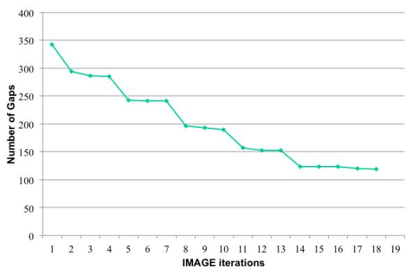
The 182 scaffolds in the E. coli assembly contain 342 gaps after being mapped to the reference genome. After 18 iterations of IMAGE, 223 of the gaps have been closed.
Figure 5.
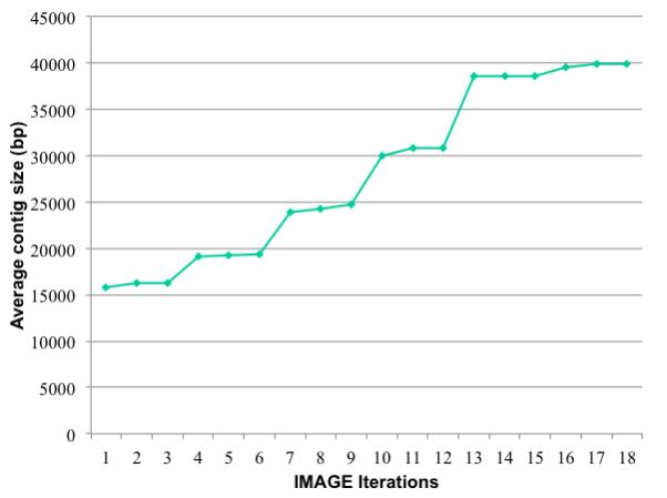
The increase in the average contig size for a series of iterations of IMAGE.
A gap closing algorithm similar to IMAGE was incorporated into the SOAPdenovo short read assembly program when it was used with the panda genome. This algorithm was able to close most of the gaps within scaffolds of the panda genome, leaving just 2.4% of the total scaffold sequence unclosed: those gaps that were unclosed either contained transposable elements (90%) or long tandem repeats 34. Other methods of gap closing involve comparing a collection of assemblies, perhaps generated with different assembly software or different sequencing technologies, in order to identify ways of extending contigs, merging or reconciling contigs, and using contigs from one assembly to bridge gaps in another. Such methods include the Graph Accordance Assembly (GAA) program 35, Reconciliator 36 and CloG 37.
Once IMAGE has closed gaps in an assembly, it can be worth attempting to calculate new scaffolding information for the new contigs as this may then define a new set of gaps for IMAGE to close. There are a number of suitable scaffolding tools available. One of the first scaffolding tools was BAMBUS 38, which can be applied to mammalian sized genomes. More recently, scaffolding tools have been developed that specifically utilise deep coverage of paired reads from second generation sequencing technologies. These include SOPRA 39, which is designed to handle SOLiD datasets for microbial genomes; SSPACE 40 which scales to mammalian sized genomes; and Opera that uses a graphical method to produce an exact solution to the scaffolding problem 41.
As well as improving whole genome assemblies, IMAGE can be used to assemble single genes of interest or to extend a known PCR-product. This is performed by generating an initial “seed” sequence of at least 300 bp. IMAGE is then used to extend the ends of the seed sequence. If the seed is initially placed like a small contig island within a scaffold gap, it may eventually merge into a larger fragment of sequence. The seed could be also a contig or supercontig of interest, as long it is longer than 300bp.
ICORN: Iterative Correction of Reference Nucleotides
ICORN 15 is designed to identify and correct small errors in consensus sequences, including errors from low-quality bases or homopolymer errors from pyrosequencing 42. ICORN cannot correct large indels or other misassemblies in consensus sequences. Every genome assembly algorithm has a unique error profile for indel errors. In general, indel errors are minimized at the expense of contig size, with aggressive assemblers generating long contigs that tend to have the most indel errors 5. ICORN works by iteratively mapping short reads against a consensus sequence to identify potential single-base discrepancies or short insertions and deletions (up to 3 bp). Before a correction is accepted, ICORN checks that it will increase the sequence accuracy by measuring the read coverage of perfectly mapping reads at that position. If the coverage is not decreased when the correction is incorporated then it is likely that the new sequence is correct. Either a user specifies a number of iterations or ICORN continues until no new corrections can be made. ICORN uses SSAHA to perform the mappings 43; the SSAHA pileup pipeline to call single nucleotide polymorphisms (SNPs) and small indels; and SNP-o-matic to evaluate potential corrections with perfect-mapping reads 44.
There are few alternatives to ICORN. Such methods include algorithms to improve base calling 45 or to detect frameshifts by protein homology or by sequence analysis. Iterative mapping approaches have been used before to derive a consensus genome sequence from metagenomic sequencing data 46 but since this derives from aggregated sequences from an unknown number of starting genotypes, the resulting consensus represents no single genome and hides much of the diversity present in the original sequence pool.
There are additional ways in which ICORN can be used. For example, it is possible to use ICORN to transform or morph a reference sequence into the sequence of an aligned comparator (e.g. reads from another strain or isolate) by “correcting” the bases over many iterations. Once ICORN has completed many iterations, all the regions of the new consensus that have average read coverage of perfect-mapping reads will represent the comparator sequence. On the other hand, those bases that are not well covered will be from the original reference sequence and should therefore be masked out. A disadvantage of this approach is that ICORN will only correct the sequence for insertions and deletions of up to 3 bp. Performing a de novo assembly is therefore necessary to find longer indels.
Another application of ICORN is to find and confirm high quality sequence variation. ICORN improves on the functionality available in the SSAHA pileup pipeline. In ICORN each variant is confirmed by perfectly mapped reads and checked and re-checked over a number of iterations. Once the sequence is corrected, new variants are often revealed that were initially obscured by the errors present in the initial sequence, while the evidence supporting other variants may have disappeared.
RATT: Rapid Annotation Transfer Tool
RATT 16 was designed to help annotate in three situations. It transfers annotation between successive versions of a genome assembly, the genomes of closely related species, or the genomes of closely related strains. Transfers are made from a high-quality reference to a new sequence by inferring “orthology” (or equivalency, in the case of successive assembly versions) and hence gene function, guided by shared synteny between the genomes. The sequences of specific genes may differ between the genomes and RATT therefore makes allowance for features such as changes to start/stop codons, the length of genes, splice sites or the presence of internal stop codons.
NUCmer from the MUMmer package 27 is used to define the sequence regions that share synteny (at least 40% sequence identity). These regions are filtered according to whether the annotation is being transferred between species, strains or genome versions. Although this function defines the synteny between blocks, it is not enough to generate a 1 to 1 relationship between bases in the reference and query sequences. However, the “show-snp” functionality from the MUMmer package is designed for identifying polymorphisms, including insertions and deletions, and it is subsequently used to refine the base-to-base relationships between the reference and query sequences.
Ambiguity may be a problem when identifying indels in repetitive regions. To overcome this RATT recalibrates the adjusted coordinates using single nucleotide polymorphisms (SNPs, also identified using “show-snp” from MUMmer) as unambiguous anchor points within synteny blocks. However, SNPs may be too rare for this if the sequences are very similar, in which case RATT temporarily modifies the query by inserting a faux SNP every 300 bp to aid in the recalibrating step: this change is reversed later so that it does not affect the final result.
Having defined the synteny blocks, the mapping stage takes place by associating each reference feature (from an EMBL file) with coordinates in the new genome. Potential mappings are ignored if a feature either (1) bridges a synteny break and if its coordinate boundaries match different chromosomes or different DNA strands or (2) if the newly mapped distance of its coordinates has increased by more than 20 kb. However, if a short sequence from the beginning, middle or the end of a feature can be placed within a synteny region, mapping is attempted.
Useful output from RATT includes information on gene models that do not map cleanly; statistics about transferred features; the amount of synteny between the reference and query; and files that allow features of the genomes to be viewed in Artemis, such as SNPs, indels and regions that lack synteny between the compared sequences.
While a number of other general automated annotation tools or pipelines do exist, such as Ensembl 47, GARSA 48 or SABIA 49, they can be relatively complex and designed for large genome sequencing centres which have an extensive network of existing software packages, servers and bioinformatics experts. Also, for microbial systems there are additional specialised software resources such as the integrated microbial genomes system 50. RATT is much simpler and more general than these approaches and is therefore more suited to the environment of a small laboratory.
Limitations and important requirements
In the flowchart shown in Figure 2 we give an overview of how subsections of the PAGIT protocol may be applied to different problems, and list the corresponding steps from the Procedure section of this article. Table 1 summarises the requirements that dictate whether a component of the protocol can be applied. If the requirement is not met, the respective component can be omitted from the protocol.
Figure 2.
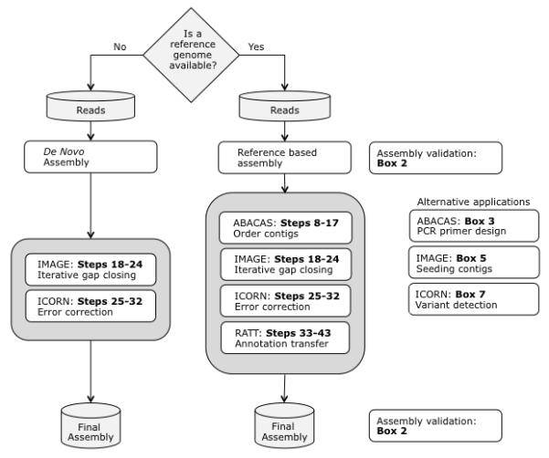
The basic workflow of the protocol is shown for two common use-cases: for de novo assembly, and when a reference genome is available. Some alternative applications of the PAGIT components are indicated. Corresponding steps from the Procedure section are listed.
Table 1.
The essential input data and hardware requirements for each software tool in the protocol. Where “Low” is given, the requirement is for much less than 1 Gb of RAM or hard disk. Please note that for larger genomes it will be essential to use parallel versions of the tools. The superscript “Para” indicates that the requirements refer to the parallel version using about 100 CPU cores.
| Genome size 4 Mbp to 25 Mbp |
Genome size several Gbp | ||||||||
|---|---|---|---|---|---|---|---|---|---|
| Reference Genome needed? |
Paired- end reads needed? |
Sequencing technology |
RAM (Gb) |
Time | Disk (Gb) |
RAM (Gb) |
Time (hours) |
Disk (Gb) |
|
| ABACAS | Yes | No | None | Low | 2 to 60 mins |
Low | 100 | 24 | 20 |
| IMAGE | No | Yes | Illumina | Up to 2 |
8 to 48 hours |
50 to 100 |
8Para | 120Para | 500Para |
| ICORN | No | Preferred | Illumina | 10 to 60 |
5 to 72 hours |
10 to 100 |
N/A | N/A | N/A |
| RATT | Yes | No | None | 2 to 6 | 2 to 30 mins |
Low | 100 | 4 to 12 | 5 |
In order for ABACAS to generate good results, the reference genome must consist of longer and more contiguous sequences than the assembly of the query genome. This will allow multiple query sequences to align to a single reference sequence: the most ideal situation is a single reference sequence or chromosome onto which many fragments from a query genome can be mapped, thus allowing the relative order of the fragments, and the gaps between them, to be defined. Preferably the reference sequences should contain fewer errors, and there should be an amino acid identity of at least 40% between the reference and query sequences.
Care should be taken to ensure that synteny is conserved between the two genomes: they should be similar enough that intra-chromosomal rearrangements are relatively minor, otherwise mapping sequences to the reference may place those sequences in an incorrect order. This needs to be considered on a case by case basis. Some bacteria, for example Wolbachia, are well known as having mosaic genomes where significant genomic rearrangements occur between species: such genomes are not suitable for use with ABACAS. Very short sequences (less than about 200bp) are difficult to place because insufficient detectable synteny will prevent ambiguous mappings from being resolved. Rearrangements between the reference and the query will be seen as long gaps, or large regions without synteny.
If the query and the reference are very similar, then after running ABACAS, all sequences should be ordered against the reference genome. Furthermore, a minimal number of larger gaps is indicative of a good quality sequence ordering. The chances of a deletion falling into a gap, or the assembler not joining the adjacent sequences, is dependent on the quality of the assembly: the fewer the gaps in the initial assembly, the lower the chance that ABACAS will introduce errors. ABACAS produces a statistics file that outputs numbers of gaps, synteny information and ordered sequences. After running ABACAS it is advisable to check for large gaps between mapped sequences, or a large quantity of unmapped sequences, as these are indicative of a low quality mapping.
Although the current implementation of ABACAS is designed to run on reference genomes with a single chromosome, it is can also be used with genomes that have more than one plasmid or chromosome (see Procedure). ABACAS uses a sensitive version of NUCmer/PROmer that could take a long time to complete for mid-size genomes with large numbers of contigs. It is therefore important to use the parameter ‘-d’ to avoid searching for repetitive regions, which will improve run-time without severely affecting sensitivity. If running on large genomes, it is important to use the 64 bit version of PAGIT. The primer design functionality of ABACAS generates high quality primers based on the uniqueness and composition of the sequence and may not always report primer sets for some regions.
The requirements for IMAGE are concerned with the availability of paired Illumina sequences with at least 20× depth of coverage. IMAGE closes the gaps between contigs in scaffolds and so scaffolds are an essential requirement. Scaffolds are a standard output from most genome assemblers, including Velvet, Newbler and Celera, and they may be created using standalone software such as SSPACE 40. Note that if the reference genome of a closely related species exists, then ABACAS can be used to generate further scaffolding information for IMAGE (by mapping the initial assembly scaffolds to the reference genome). However, it is important to check that the scaffolding information is correct or else IMAGE may close false gaps or no gaps in the assembly. Depending on the repetitive nature of the genome, assembly quality and the coverage depth of the paired-end reads used by IMAGE, up to 50% of gaps can be closed. When using Illumina data, IMAGE can only run with paired-reads with inserts of a few hundred base pairs.
ICORN will perform best if the coverage of the genome is between 20-60× and distributed evenly over the complete genome. In this case most of the bases will be successfully corrected, although repetitive regions where reads cannot be mapped unambiguously will not. General systematic errors in short reads are not possible to correct. For example, long homopolymer tracks with more than 10 bases are often sequenced erroneously by Illumina technology 15.
If a genome is larger than 6 Mb or if coverage exceeds 200×, then ICORN might perform slowly and need a relatively high amount of memory (up to 15 GB). For a bacterial genome of around 4 Mb in size, with 100× of coverage, each iteration should take less than an hour. Up to 5 iterations are typically performed with about 80% of the errors corrected in the first iteration.
RATT requires an annotated reference genome for its input. The proportion of synteny between the reference genome and the new genome corresponds to the proportion of genes that can be transferred. The sequence identity to transfer the annotation should be over 40% for at least 50 bases upstream and downstream from the annotated feature. Gaps in either the reference genome or the new genome will adversely affect performance. For regions in which no synteny exists no transfer can be carried out and the user will then need to do ab initio gene finding and functional annotation3, perhaps using gene prediction software such as Augustus 51. Such unannotated regions are flagged and written to a file that can be loaded onto the new reference. For bacterial sized genomes RATT uses around 1 Gb of RAM and runs in around 5-10 minutes, while for malaria-sized genomes (about 23 Mb) it requires up to 6Gb of RAM and 10-30 minutes.
Scalability issues
PAGIT was mainly designed for working on parasite genomes of up to about 300 Mb. In this protocol we have emphasised its applicability to smaller genomes, which can be worked on relatively quickly and simply without the need for parallelisation or specialised computing infrastructure. However, it is worth noting that the tools may be used on significantly larger genomes if such infrastructure is available.
ABACAS and RATT both rely on MUMmer tools to perform their alignments, and when run in the default 32-bit mode this limits the size of the genomes being aligned to about 200-300 Mb. However, when MUMmer is compiled in a 64-bit mode this limitation no longer applies – as long as enough RAM is available to handle the larger genome alignments. To reduce the runtime it is also advisable to use larger seeds in the alignments, which are controlled via the ABACAS “-s” parameter. For example, using ABACAS to order contigs from an assembly of mouse chromosome 1 against the complete mouse genome required almost 100 Gb of RAM and took about 4 hours. To transfer with RATT a subset of the annotation of the Human genome to the Chimp genome required 60 Gb of RAM and took about 70 minutes. These tests were performed using an Intel Xeon 2.40 GHz E7440 processor.
IMAGE and ICORN do not scale so easily in the serial implementations, as we have discussed in this paper. The IMAGE and ICORN serial implementations are currently unsuitable for genomes larger than about 25 Mb. Much of their limitation comes from the large numbers of reads that need to be mapped. For small genomes, reads can usually be mapped in hours using a single processor, but for larger genomes this can take weeks, and then it is highly desirable to speed up this process by using a high-throughput computing resource. IMAGE is also limited by the numbers of gaps that must be closed: many gaps means that many local assemblies must be performed to close those gaps. Versions of IMAGE and ICORN that are able to parallelise tasks via the Platform LSF cluster management system are available from the SourceForge websites of these tools (which are linked to from the PAGIT website). For the parallel versions, IMAGE can scale up to genomes Gigabytes in size (it has been used on mouse) and ICORN can be applied to genomes of up to approximately 300 Mb.
Expected improvements
Sequencing technologies are rapidly evolving and the tools comprising the PAGIT protocol are continuously under development in order to adapt to those changes. In future ABACAS should be able to join two neighbouring contigs, if they overlap with at least 50 bases and no mismatches. IMAGE will support newer sequencing technologies such as the PacBio RS from Pacific Biosciences or Ion Torrent, while improvements to ICORN will allow different tools to be used to map reads and call variants (with significantly lower memory requirements than the currently used SSAHA pileup pipeline). Finally, future developments for RATT are concerned with accurately transferring greater numbers of genes between species that are more distant.
Materials
EQUIPMENT
Hardware and software
The protocol is designed for a Linux environment. Depending on the size of the target genomes different requirements may arise, as discussed in the preceding sections. For genomes of up to 200 Mb, a machine with about 16 Gb of RAM and about 50 Gb of free disk space could be sufficient. The whole pipeline should complete in about one day for microbial genomes, or several days for larger genomes (a computer cluster may be required).
There are two ways to run PAGIT: as Linux binaries (recommended) or as a preinstalled Linux version running under a virtual machine. The virtual machine can run under MAC OS or Windows and should be sufficient for genomes of up to 3 Mb. We have precompiled Linux and virtual machine versions of PAGIT for 32bit and 64bit systems. The 64 bit virtual machine should be able to access more RAM and may therefore be suitable for larger genomes.
For the Linux version, a bash-shell must be running, and a tcsh-shell and Java version 1.6 (http://www.java.com/en/download/manual.jsp) must be pre-installed.
For the virtual machine version, the virtual box software from VirtualBox must be downloaded and installed. This process is well documented at https://www.virtualbox.org/wiki/Downloads
PAGIT is available from http://www.sanger.ac.uk/resources/software/pagit/.
Procedure
Obtaining and installing PAGIT Timing 15 to 45 minutes
(1) There are two recommended ways to install PAGIT, depending on the available operating system. Follow option A for Linux or option B for Windows or MAC OS:
(A) Linux
(i) Download the appropriate compressed tar archive for your Linux system. Click on either the “Linux binary x32bit” or the “Linux binary x64bit” link from the “Download” tab of the PAGIT website: http://www.sanger.ac.uk/resources/software/pagit/.
(ii) Move the compressed tar archive to the location where you want PAGIT installed, then decompress the tar ball by typing the following commands in a terminal window:
mv PAGIT.V1.64bit.tgz /path/to/my/installed/software
cd /path/to/my/installed/software
tar xzf PAGIT.V1.64bit.tgz
(iii) Execute the install script by typing the following in a terminal window:
bash ./installme.sh
(iv) Switch to bash-shell
bash
(v) Source the environment settings to run PAGIT:
source PAGIT/sourceme.pagit
Critical Step
The environment settings for PAGIT should be sourced each time PAGIT is executed. Alternatively, the command “source PAGIT/sourceme.pagit” may be included into your local environmental variable file (for example the file “~/.bashrc”) so that the PAGIT environment is automatically initialised.
(B) Windows or MAC OS
If not already performed, download the virtual box software from VirtualBox and install it according the VirtualBox documentation: https://www.virtualbox.org/wiki/Downloads
Download the PAGIT virtual machine required for your Linux system. Click on either the “Virtual Machine 32 bit” or the “Virtual Machine 64 bit” link from the “Download” tab of the PAGIT website:http://www.sanger.ac.uk/resources/software/pagit/.
Register the downloaded PAGIT virtual machine. Open virtual box and click on new to create a new virtual machine. Click on “next” to move through the registration screens.
Name the virtual machine (e.g. PAGIT) and select the operating system and version: “Linux” and then either “Ubuntu” or “Ubuntu64”.
Specify the amount of memory to be allocated. You shouldn’t give the virtual machine more than 75% of the complete memory available, but it should have at least 2GB.
Specify the Virtual Hard Disk using the toggle on the “use existing hard disk” option and click on the file icon to find and select the downloaded PAGIT virtual machine. (“Start-Up Disk” should be enabled.)
To start the virtual machine, select it and click on the green arrow.
(2) Running the PAGIT test example: Move to the PAGIT test example directory by typing the following in a terminal window:
cd $PAGIT_HOME/exampleTestset/
(3) Run the test by typing the following in a terminal window:
bash ./dotestrun.sh
(4) Initial setup of input files: make a working directory for PAGIT. Type the following command in a terminal window:
mkdir myWorkingDir
(5) Either copy the initial assembly, or to make a symbolic link from it to the working directory type the following commands in a terminal window:
cd myWorkingDir
ln –s /path/to/assembly/scaffolds.fasta ./assembly.fasta
Critical step
Before proceeding with assembly improvements, it may be worth validating the quality of the initial assembly. Methods of doing this are given in BOX 2.
BOX 2. Assembly validation using ICORN and Artemis.
Genome assembly algorithms often misassemble fragments of a genome5, 9. Many of these mistakes cannot currently be corrected automatically, however software for evaluating and identifying potential misassemblies has been developed52. Here we describe a few ways in which ICORN and Artemis can be used to check and evaluate the consensus sequence.
(1) The following approach can be used to check if certain regions in the genome are not covered by perfectly mapping reads (a read and its mate are considered “perfecty mapping” if they are identical to the reference and their mapping distance is in the expected insert size). The “getPerfectCoverage.2lanes.sh” script uses the very fast SNP-o-MATIC algorithm to generate plot files for each sequence in a given file. It should take about five minutes for bacterial genomes. The arguments to the script are: the genome sequence; the first Illumina FASTQ file; the second Illumina FASTQ file; and the mean fragment size for the paired Illumina reads. Standard output should indicate the coverage levels. Plots for each sequence can be found in the output directory “PerfectCoverageplots”. Type the following command in a terminal window:
getPerfectCoverage.2lanes.sh finalICORNresult.fasta pairedReadsPart_1.fastq
pairedReadsPart_2.fastq 300
The generated plots can be loaded into Artemis. Possible problems with the assembly are indicated where the coverage drops toward zero. Then using the logarithmic view, the sink in the plots are more visible.
Please note that SNP-o-MATIC maps a repetitive mapping read pair to all the possible positions in the genome. This means that if a repetitive region is represented 3 times in a genome, the coverage would be tripled as compared to the rest of the genome.
(2) Possible mis-assemblies can be found in regions with 0 or <5 perfect mapping reads. Those potential erroneous regions can be converted to a sequencing gap (i.e. the bases are switched to N’s). Rather than do this manually in Artemis, it is easiest to use the “PerfectMapping2n.pl” script, with the directory “PerfectCoverageplots” generated by the “getPerfectCoverage.2lanes.sh” script (described above), to generate a new fasta file, “result.fasta”. Type the following in a terminal window:
PerfectMapping2n.pl finalICORNresult.fasta PerfectCoverageplots result.fasta
The standard output will report how many bases were converted to N’s. For all further downstream analysis it is recommended to use this output. Please note that this script could also be run on an initial assembly, or on the output from ABACAS, so that the regions converted to N’s could subsequently be closed by IMAGE. The only drawback could be that few reads map close to the ends of contigs, and therefore the gaps might be extended.
Please note that although the script can find mis-assemblies, it cannot be guaranteed to find them all.
(3) Another option to investigate the quality of the consensus sequence is to map the sequencing reads back to it and visualize the resulting BAM file in Artemis or ACT (a BAM file contains all mapping information for all the reads). PAGIT has a script to map the reads with SMALT (http://www.sanger.ac.uk/resources/software/smalt/) against the given reference and generate a BAM file called “little.smalt.bam.sh”. The first parameter is the sequence file, followed by the k-mer and step size for SMALT. We suggest leaving those as given in this example. Next the forward and reverse reads are given. The last two parameters are the output prefix for the mapping results and the insert size of the read-pairs:
little.smalt.bam.sh finalICORNresult.fasta 15 3
pairedReadsPart_1.fastq pairedReadsPart_2.fastq ResultMapping 1000
To open the BAM file in Artemis, type:
art -Dbam=ResultMapping.bam finalICORNresult.fasta
Visualising mapped reads is a powerful way to analyse the data. For example, it is possible to check if the coverage over the ABACAS bin contigs (i.e. the contigs that weren’t aligned against the reference) is equal to that of the rest of the assembly – contamination and new plasmids have different coverage levels. It is possible to examine if the two mates are mapping on different contigs, and then it might be appropriate to order (i.e. scaffold) the contigs manually. Smaller regions of higher coverage could indicate collapsed repeats. Regions with heterozygous SNP’s (such that not all reads have the SNP) in haploid genomes can indicate indels. For examples please see http://www.sanger.ac.uk/resources/software/artemis/ngs/.
(6) Either copy the read libraries, the reference genome sequence, and the reference genome annotation, or to link them to the working directory type the following commands in a terminal window:
ln –s /path/to/reads/readLibraryPart_1.fastq .
ln –s /path/to/reads/readLibraryPart_2.fastq .
ln –s /path/to/reference/Refsequence.fasta .
ln –s /path/to/reference/Refannotations.embl .
(7) (Optional) Find reference annotations online through searching the “Genome” database at the NCBI (http://www.ncbi.nlm.nih.gov) and then convert the NCBI annotations, which are in Genbank format, to EMBL format. There are a number of ways to convert annotations (one easy way is to load the Genbank file into Artemis and save it as an EMBL entry, but here we use a bioperl script available from the RATT website to perform the conversion. There are two arguments to the script: the first is the Genbank annotations, the second the output file with the annotations in the EMBL format:
genbank2embl.pl Refannotations.gbk Refannotations.embl
Critical step
Alternatively, annotations are stored at the EBI (http://www.ebi.ac.uk) in EMBL format with the same accession numbers as used by the NCBI.
Running ABACAS to order contigs or scaffolds on a reference genome Timing 10-20 mins
(8) Setup a working directory for ABACAS, and link in the files containing the genome assembly and the reference genome by typing the following commands in a terminal window:
cd /path/to/myWorkingDir
mkdir runABACAS
cd runABACAS
ln –s ../assembly.fasta .
ln –s ../Refsequence.fasta .
Critical step
ABACAS can also be used for primer design as described in Box 3.
Box 3. Running ABACAS for primer design.
(1) After the contig ordering is completed, ABACAS will prompt users to provide appropriate parameters for selecting primers. These parameters include primer size, melting temperature, size of flanking regions, product size and GC content of primers. Primers can be automatically designed while ordering contigs using the following command:
perl $PAGIT_HOME/ABACAS/abacas.pl –r Refsequence.fasta -q assembly.fasta -p nucmer -m –b –o myOutput –P
Critical step
Sequence gaps represented as “N”s (as small as 1bp) will be identified by ABACAS for primer design. It is therefore important to check the distribution of gap sizes prior to setting the maximum product size.
? TROUBLESHOOTING
(2) Primer design can also be performed independently after the contig ordering stage. Here the flag “–e” dictates that ABACAS will ignore the sequence ordering step and go directly to designing primers. Primer sets are checked for uniqueness against the reference genome using a sensitive NUCmer search. The primer design phase could be repeated for different parameters without re-ordering contigs. To perform this type the following command in a terminal window:
perl $PAGIT_HOME/ABACAS/abacas.pl –r Refsequence.fasta -q assembly.fasta –e
? TROUBLESHOOTING
(3) Check the ABACAS output. Sense and antisense primers are written in separate files formatted using a 96 well plate: “sense_primers.out” and “antiSense_primers.out”. Other output files include a primer3 summary file with alternative primer sets: “antiSense_primers.out”. See Box 4 for further information on ABACAS output.
(4) ABACAS can also be used to design primers to validate SNPs from functional studies by replacing each putative SNP position with 5 N’s, so ABACAS assumes they are gaps and therefore will design primers over the regions.
(9) (Optional) If there are multiple chromosomes, plasmids, or other sequences in the reference file, then, before ABACAS is executed, these must be joined in such a manner that they appear to be a single reference sequence. After the alignment, the mapped contigs can be subdivided according to the reference sequences they were mapped against (Step 11). Type the following command in a terminal window to join the reference sequences into the file “Refsequence.union.fasta”. This file should now be used in place of the file “Refsequence.fasta” in subsequent steps:
perl $PAGIT_HOME/ABACAS/joinMultifasta.pl Refsequence.fasta
Refsequence.union.fasta
(10) Check ABACAS usage information and view basic help, then run ABACAS with the required parameters. The main parameters are: the “–r” flag that is used to specify the file containing the reference genome; the “–q” flag that specifies the file containing the assembled sequences that are to be ordered; the “–p” flag that specifies which alignment program to use: either NUCmer for alignment in nucleic acid space or PROmer for alignment in amino-acid space; and the “–o” flag that specifies the prefix for the output file names. The default options generate ordered contigs in a single FASTA file. However, using flags “–m” and “–b”, multiple-FASTA format files of the ordered contigs and the unused contigs (from the bin) can be produced. Call ABACAS by typing the following commands in a terminal window:
perl $PAGIT_HOME/ABACAS/abacas.pl -h
perl $PAGIT_HOME/ABACAS/abacas.pl -r Refsequence.fasta -q
assembly.fasta -p nucmer -m –b –o myPrefix
Critical step
If you have a circular genome you can use the “-c” flag.
! CAUTION
Errors may occur if two or more instance of ABACAS are running in the same directory. This is because the alignment software NUCmer or PROmer always outputs a temporary file with the same name, and so multiple instances of ABACAS will attempt to read and write from the same file. Only run a single ABACAS instance in a directory at a time.
? TROUBLESHOOTING
(11) (Optional) If you ran the “joinMultifasta.pl” script (Step 9) before running ABACAS, then you will need to use the “splitABACASunion.pl” script to decompose the results into contig mappings against the individual reference sequences. The results will be “myPrefix.ReferenceName.fasta” and “myPrefix.ReferenceName.tab”, where “ReferenceName” stands for the replicon names from the reference. Type the following command in a terminal window, where the three files beginning with “myPrefix” will be the output from the ABACAS run:
perl $PAGIT_HOME/ABACAS/splitABACASunion.pl Refsequence.fasta
Refsequence.union.fasta myPrefix.fasta myPrefix.crunch myPrefix.tab
(12) Check ABACAS output (see Box 4). To gain a general overview of the results, first look at the file “myPrefix.gaps.stats”. This file provides a quick summary of the gaps present in the ordered pseudomolecule. Type the following command in a terminal window:
Box 4. Output interpretation for ABACAS.
To gain a quick overview of the output of ABACAS look at the file “myPrefix.gaps.stats”. This file gives statistics about the gaps that remain in the assembly after mapping it to the reference. These include the number of overlapping gaps and the number of real gaps; and then further statistics on the real gaps, such as the minimum, maximum and median gap size, the sum of all the gaps and the N50 gap size.
Two types of gaps are considered in the output of ABACAS. Real gaps are regions of the reference genome where no contigs map. Overlapping gaps are derived from two contigs that map to the genome and which overlap in their mapped positions, often due low quality sequences at the ends of contigs. A gap is therefore inserted between the mapped contigs and can subsequently be closed by running IMAGE. ABACAS introduces 100 Ns (or a number specified by the user using flag “-g”) to distinguish such gaps from real or genuine gaps.
To gain a clearer view of the contig mapping, ABACAS produces output files that may be visualised using a genome browser like Artemis or ACT. These files include:
myPrefix.crunch: this is the main file to be used by a genome browser. The format is standard for genome browsers and described in the Artemis manual.
myPrefix.tab: this is a genome browser feature file and it gives colour-coded mapping information that describes if the contigs align in a forward or reverse direction, or they are overlapping.
myPrefix.gaps.tab: this is a genome browser feature file that describes the length and type of gaps (i.e. overlapping or real gaps).
Other output files list some general information about the contig mappings:
myPrefix.gaps: each line in this file describes one of the gaps. The columns in this file are as follows: the first is always the text “Gap”. The second is the size of the gap. Columns 3 to 6 represent start and end positions on the pseudomolecule and then start and end positions on the reference. The final column describes if the gap is a non-overlapping (i.e. real) gap, or if it is a gap introduced due to overlapping contigs. A quick overview of gap sizes can be found from the second column of the *.gaps output file (awk ‘print $2 ‘ *.gaps). Extracting this column to a file will allow for quick statistics of the gaps using R or excel.
myPrefix.bin: a list of unmapped contigs.
myPrefix.fasta: this is the output sequence i.e. the contigs mapped to the chromosome or chromosomes with the gaps denoted by a series of Ns.
Please note that ABACAS has various parameters that may be used to control the output, as described in its usage information.
more myPrefix.gaps.stats
! CAUTION
ABACAS is not designed to order genomes where rearrangement is expected, as it might result in the wrong order of contigs. Large gaps listed in the file “myPrefix.gaps.stats” can indicate possible rearrangements between the genomes.
(13) (Optional) To visualise the mapped alignments using the ACT genome browser type the following command in a terminal window:
act Refsequence.fasta myPrefix.fasta.crunch myPrefix.fasta
(14) (Optional) To view other ABACAS output files in ACT such as feature files describing ordered contigs and gaps (“myPrefix.tab” and “myPrefix.gaps.tab”), then in ACT go to File > Read an entry, and select “myPrefix.gaps.tab”.
(15) (Optional) Unmapped contigs will be placed in the ABACAS bin: it is recommended to BLAST the contigs in the bin against the reference by using ABACAS with the “–b –t” options. If the binned contigs have acceptable matches with the reference according to the BLAST results, then the ordering parameters used by ABACAS may have been too strict. It is therefore recommended to re-run ABACAS with slightly less stringent parameters, or to improve the ordering by moving contigs around using a genome browser such as ACT. In ABACAS, the option “-a” will append the bin contigs at the end of the pseudomolecule and these will then be visible in ACT for manual adjustment. This option is not recommended if IMAGE will be run subsequently, as the contig borders will be lost.
! CAUTION
The contigs in the bin may contain important biological information, such as strain-specific insertions, plasmids or highly diverged sequence, which might be worth further investigation.
(16) (Optional) The crunch file generated through NUCmer or PROmer is not as accurate as a BLAST comparison file; however it is possible to generate a BLAST comparison file. To do this, first create a blast database from the reference genome; then BLAST the mapped contigs against the created BLAST database; and finally start up ACT. Type the following commands in a terminal window:
formatdb -p F -i Refsequence.fasta
blastall -p tblastx -e 1e-20 -m 8 -d Refsequence.fasta -i
myPrefix.fasta -o myPrefix.blast
act Refsequence.fasta myPrefix.blast myPrefix.fasta
Critical step
To obtain a nucleotide comparison rather that a six frame comparison, change “TBLASTX” to “BLASTN”.
(17) In preparation for running IMAGE, concatenate together the mapped sequences and the unmapped sequences. Type the following command in a terminal window:
cat myPrefix.fasta myPrefix.contigsInbin.fasta >
mappedAndUnmapped.fasta
! CAUTION
If this concatenation step is skipped (or if the “–b” option is not used with ABACAS) then the unmapped sequences of the genome will be lost to subsequent steps of the protocol. Note that the “-a” option should not have been used, because the unordered contigs would be part of ordered the pseudo molecule.
Running IMAGE to close gaps in scaffolds Timing approximately 6 hours
(18) Setup a working directory for IMAGE, and link in the files containing the short read pairs by typing the following commands in a terminal window:
cd /path/to/myWorkingDir
mkdir runIMAGE
cd runIMAGE
ln –s /path/to/pairedReadsPart_1.fastq .
ln –s /path/to/pairedReadsPart_2.fastq .
! CAUTION
Before running IMAGE (or generally doing assemblies), sequencing reads should be cleaned from possible sequencing vector, as they can generate assembly errors. Reads can be trimmed or removed from the read set e.g. using Cutadapt (http://code.google.com/p/cutadapt/).
Critical step
IMAGE can also be used for extending seed sequences into longer contigs as described in Box 5.
Box 5. Using IMAGE for extending seed sequences into longer contigs.
(1) Setup a working directory for IMAGE, and link in the files containing the seed sequences, and the read pairs by typing the following commands in a terminal window:
cd /path/to/myWorkingDir
mkdir runIMAGE
cd runIMAGE
ln –s /path/to/pairedReadsPart_1.fastq .
ln –s /path/to/pairedReadsPart_2.fastq .
ln –s /path/to/seed.fasta
! CAUTION
The initial seed sequences must be of at least 300 bp.
(2) Run IMAGE using the “-smalt_minScore” parameter and specify a relatively large number of iterations. The “-smalt_minScore” parameter is used to specify the Smith-Waterman score that a read has when mapped onto the reference: if it maps with its complete length, without any mismatch or indel, then the score is equal to the read length; whereas if it maps with one mismatch, then the score is the read length minus 3. Therefore, to map the reads to positions where each read would be expected to have 3 mismatches, the “-smalt_minScore” parameter would be set to the read length minus 9. In this way the “-smalt_minScore” parameter is used to tighten the constraints on where a read is mapped to a contig – and it therefore determines if the second read of the pair is able to extend the contig and thus should be included in a local assembly. Type the following command in a terminal window (for 75bp reads):
perl $PAGIT_HOME/IMAGE/image.pl -scaffold seed.fasta -prefix
pairedReadsPart -iteration 1 -all_iteration 30 -dir_prefix ite_seed -smalt_minScore 67 –kmer 71
Critical step
It is important that the mapping constraints are tight enough to ensure that reads from different regions of the genome do not map to the seed.
Critical step
It is best to use large k-mers for seeding applications.
! CAUTION
If the seed is similar to another region of the genome then this approach may create a chimeric contig.
? TROUBLESHOOTING
(3) To check the results using the “image_run_summary.pl” script, as described in Step 22, type the following command in a terminal window:
perl $PAGIT_HOME/IMAGE/image_run_summary.pl ite_seed
(19) To link in the latest assembly, either the output from ABACAS (from Step 17) or the sequence output from a de novo assembly, type the following command into a terminal window:
ln –s /path/to/assembly inputScaffolds.fasta
(20) Check IMAGE usage information and view basic help, by typing the following command in a terminal window:
perl $PAGIT_HOME/IMAGE/image.pl
! CAUTION
It can be a good idea to remove smaller contigs (less than 500bp) from the assembly before running IMAGE. If a contig should have been placed in the gap of a scaffold or a pseudo molecule, but wasn’t, then it is just possible to close this gap by deleting the small contig.
(21) Run IMAGE with the required parameters by executing one of the following sets of commands; option A represents the simplest usage, while option B optimizes the gap closing. In the following, the “–scaffolds” option defines an input file in FASTA format of sequences containing gaps to be closed; the “–prefix” option identifies the fastq files containing the read pair sequences; the “– dir_prefix” option gives the directory name prefix for the directories containing the output files for each iteration, the option “–iteration” specifies the number of the first iteration, and the “– all_iteration” option defines the range or total number of iterations. These numbers are combined with the directory prefix to create the names of the output directories. Finally, the “–kmer” option specifies the k-mer used for the local assemblies performed at the gaps:
(A) The simplest usage of IMAGE
(i) To use a single k-mer and run through a number of iterations without restarting, type the following command in a terminal window:
perl $PAGIT_HOME/IMAGE/image.pl -scaffolds inputScaffolds.fasta –
prefix pairedReadsPart -iteration 1 -all_iteration 9 -dir_prefix ite –kmer 55
? TROUBLESHOOTING
(B) Optimizing the gap closing
(i) If the reads used to span the gaps are relatively large (for example 108 bp) then the results from IMAGE can be improved by using a range of different k-mers. To run IMAGE with a range of k-mers, type the following commands in a terminal window:
perl $PAGIT_HOME/IMAGE/image.pl -scaffolds inputScaffolds.fasta –
prefix pairedReadsPart -iteration 1 -all_iteration3 -dir_prefix ite –kmer 91
perl $PAGIT_HOME/IMAGE/restartIMAGE.pl ite3 71 3 partitioned
perl $PAGIT_HOME/IMAGE/restartIMAGE.pl ite6 51 3 partitioned
perl $PAGIT_HOME/IMAGE/restartIMAGE.pl ite9 31 3 partitioned
Critical step
Note that the initial iterations of IMAGE close the most gaps, especially the first and second iterations. If time or computational resources are limited then just running 1 or maybe 2 iterations with a small k-mer can still significantly improve a genome assembly.
? TROUBLESHOOTING
(22) Check the output of IMAGE (see Box 6). In each iteration directory (these directories are called after the value given to the “–dir_prefix” parameter) there is a file called “walk2.summary” which contains some statistics describing what was achieved during that gap closing iteration. A summary of the statistics in each of these files may be viewed by using the “image_run_summary.pl” script, which has only one argument: the prefix of the output directories. To run the script type the following commands in a terminal window:
BOX 6. Output interpretation for IMAGE.
IMAGE outputs a relatively large number of files when it is running, but only a small number need be of interest to the user: these files are located in each of the iteration directories. Within each IMAGE iteration directory three of the files created are of particular interest. These files include:
new.fa: the set of updated contigs created during the current gap closing iteration.
new.read.placed: maps contigs to scaffolds, for the current iteration.
walk2.summary: gives a short description of the gap closing results for each iteration, including the number of gaps in the assembly, the number closed during the current iteration, and contigs that have been extended from one or both sides.
After the first iteration, IMAGE creates a much smaller subset or partition of each of the initial FASTQ files. These new FASTQ files (“partitioned_1.fastq” and “partitioned_2.fastq”) only contain those reads that are involved in spanning gaps (i.e. read pairs that map to the middle of contigs are removed). When the initial FASTQ files are very large, using the partitioned FASTQ files can significantly reduce the execution time.
IMAGE provides scripts that summarise the output from all iteration directories (i.e. the gaps closed, extended and so on) and that re-scaffold the final set of contigs (“image_run_summary.pl” and “contigs2scaffolds.pl”).
In the base IMAGE directory, when IMAGE is executed using the “–scaffolds” option, the following input files for IMAGE are automatically created:
read.placed.original: maps contigs to scaffolds for the initial FASTA file (that contains sequences with gaps to be closed).
read.placed: may rename the contigs and scaffolds in the read.placed.original file if they contain problematic characters.
contigs.fa.original: contains the initial set of contig sequences in FASTA format.
contigs.fa: may rename the contig headers in the contigs.fa.original file if they contain problematic characters.
Critical step
If another run of IMAGE is started using the “image.pl” script in the same directory as an existing IMAGE run, then it is important to first delete the automatically created input files because IMAGE will not overwrite them. Please note that the recommended way to continue an existing IMAGE run is via the “restartIMAGE.pl” script: it is not necessary to delete any files before running this script.
perl $PAGIT_HOME/IMAGE/image_run_summary.pl
perl $PAGIT_HOME/IMAGE/image_run_summary.pl ite
(23) (Optional) If the output of IMAGE shows that gaps are still being closed, or if contigs are still being extended, then it may be worth running some more iterations. To restart IMAGE from iteration 9, with a k-mer size of 31, for 3 more iterations, type the following into a terminal window:
perl $PAGIT_HOME/IMAGE/restartIMAGE.pl ite9 31 3 partitioned
? TROUBLESHOOTING
(24) Once IMAGE has completed its run, the contigs that are found in the file “new.fa” under each iteration directory may be output as scaffolds using the “contigs2scaffolds.pl” script. See Box 6 for further detail about IMAGE output. The final iteration directory (i.e. the directory with the highest number appended to its prefix name, e.g. “ite9”) gives the most contiguous set of contigs. The arguments given to the “contigs2scaffolds.pl” script are as follows: “new.fa” is the file containing the set of contigs for the final iteration; the file “new.read.placed” gives the scaffolding information for the new contigs based on the initial set of scaffolds; the number “300” gives the gap between contigs in the scaffold (denoted by NNs in the output file), “0” gives the minimum size for contigs to be included in the scaffolds output file; and “scaffolds” is the prefix of the output scaffolds file which will be in FASTA format. Type the following commands in a terminal window to change to the final iteration directory, to view the usage information for the script “contigs2scaffolds.pl”, and to run the script:
cd ite9
perl $PAGIT_HOME/IMAGE/contigs2scaffolds.pl
perl $PAGIT_HOME/IMAGE/contigs2scaffolds.pl new.fa new.read.placed
300 0 scaffolds
! CAUTION
In some applications we have observed small contigs (<=500bp) generating miss-assemblies by duplicating their sequence.
Running ICORN to correct small insertions and deletions as well as single base-pair errors Timing 1 hour per iteration
(25) Setup a working directory for ICORN, and link in the files containing Illumina reads by typing the following commands in a terminal window:
cd /path/to/myWorkingDir
mkdir runICORN
cd runICORN
ln –s /path/to/pairedReadsPart_1.fastq .
ln –s /path/to/pairedReadsPart_2.fastq .
Critical step
ICORN can also be used to find high quality variants as described in Box 7.
Box 7. Using ICORN to find high quality variants.
(1) Setup a working directory for ICORN, and link in the files containing Illumina reads and the sequence to be investigated for variants by typing the following commands in a terminal window:
cd /path/to/myWorkingDir
mkdir runICORN
cd runICORN
ln –s /path/to/pairedReadsPart_1.fastq .
ln –s /path/to/pairedReadsPart_2.fastq .
ln –s /path/to/sequence.fasta uncorrected.fasta
(2) Call ICORN by typing the following commands in a terminal window:
ICORN.start.sh uncorrected.fasta 1 6 pairedReadsPart_1.fastq pairedReadsPart_2.fastq 100,500 250
? TROUBLESHOOTING
(3) Check the output file ending in “.PerBase.stats” to obtain a list of the variants that ICORN found for each iteration. This is described in Box 8.
(4) (Optional) If the results are satisfactory then the ICORN output can be removed. Delete all the directories generated by ICORN by typing the following command in a terminal window:
rm -r Reference.*/
(26) Link in the assembly to be corrected. This could be the output from ABACAS (from Step 17) or IMAGE (from Step 24), or the sequences output from a de novo assembly. Type the following command into a terminal window:
ln –s /path/to/assembly uncorrected.fasta
(27) First check ICORN usage information and view basic help. The arguments to ICORN are as follows: the first is the FASTA file of the sequence to be corrected; the second and third specify the first and last iterations; then come the Illumina read file or files used to make the corrections. For paired-end reads a number of libraries can be used. A file is specified for each half of the pair, followed by an estimation of the range of the insert size for the paired reads and the mean insert size range; if another paired-end Illumina library is available, then this is specified in the same way. If a single-end library is available then the insert size arguments are missed out. Type the following command in a terminal window:
icorn.start.sh
(28) Run ICORN with the required parameters. Choose one of the following options, depending on the available Illumina libraries; use option A to call ICORN with one paired-end library, option B if two paired-end libraries are available, or option C if only one single-end Illumina library is available:
(A) To call ICORN with one paired-end library (with an insert size of 250bp)
(i) Type a command similar to the following in a terminal window:
icorn.start.sh uncorrected.fasta 1 6 pairedReadsPart_1.fastq
pairedReadsPart_2.fastq 100,500 250
? TROUBLESHOOTING
(B) To call ICORN if two paired-end libraries are available (with insert sizes of 250bp and 3000bp)
(i) Type commands similar to the following in a terminal window:
icorn.start.sh uncorrected.fasta 1 6 ApairedReadsPart_1.fastq
ApairedReadsPart_2.fastq 100,500 250 BpairedReadsPart_1.fastq
BpairedReadsPart_2.fastq 2000,4000 3000
? TROUBLESHOOTING
(C) To call ICORN if only one single-end Illumina library is available
(i) Type a command similar to the following in a terminal window:
icorn.start.sh uncorrected.fasta 1 6 unpairedReads.fastq
? TROUBLESHOOTING
Critical step
If you have long insert size libraries it might be necessary to reverse complement the reads before performing the mapping.
(29) At the end of an ICORN run, three small files may be consulted to view how ICORN has performed: the “ICORN.overview.txt“ file has a general overview; the “Stats.Mapping.csv” file shows the improvements in the number of reads that map to the sequence after each iteration; and the “stats.Correction.csv” file that gives the numbers of corrections made for each iteration. For further detail please see Box 8. To view the contents of these files, type the following commands in a terminal window:
BOX 8. Output interpretation for ICORN.
If ICORN runs to completion there will be a directory for each ICORN iteration. The names of these directories are based on the original sequence file, with a number appended to the original file name corresponding to each iteration.
In the main ICORN working directory there are two important files to look at after a run:
Stats.Mapping.csv: statistics based on the number of reads mapped (including read-pairs and unique mappings), the depth of genome coverage of the mapped reads, and how the genome size may change as corrections are made due to small insertions and deletions. There is a separate column of results for each ICORN iteration.
- Stats.Correction.csv: a break-down of the different types of correction made by ICORN. A separate column is given for each ICORN iteration. The types of correction made by ICORN are as follows:
- SNP: the correction of a single nucleotide or base pair
- INS: inserted up to 3 base pairs in order to fix an incorrect deletion
- DEL: removed up to 3 base pairs in order to fix an incorrect insertion
- HETERO: If a second allele is called with a frequency between 0.15 - 0.5, the base is called heterozygous. The consensus sequence is derived from the most abundant allele.
- Three types of correction (SNP, INS and DEL) that are themselves corrected (i.e. rejected) as the coverage of mapping reads increases. The corrections are labelled as Rej.SNP, Rej.INS, and Rej.Del.
To see a summary of the ICORN results, look at the file “ICORN.overview.txt”. This file contains basic information on the corrections, and the coverage of mapping reads. It is a short summary of the above two files, including amount of corrections per iteration and amount base covered with perfect mapping reads.
Around 90% of the reads should map, depending on the quality of the Illumina input files and the draft genome. For read pairs, the amount of uniquely mapped read pairs should be 60-80%, although a repeat-rich genome may reduce this substantially. If a newly generated draft genome is used, then this number may drop to around 40% as most read pairs will lie on different contigs. Just regions covered with 20× mapped reads will be corrected.
Using a genome browser such as Artemis and the GFF files output by ICORN it is possible to view the corrections made for each sequence (contigs or scaffold) in the uncorrected input file. GFF files are made at each iteration, and at the end of the iterations these files are combined into a single file (for each contig or scaffold). The naming convention for these files is as follows:
At each iteration the GFF files are made from three components joined together using a “.”: the initial uncorrected sequence name (e.g. “uncorrected.seq”), the iteration number (e.g. 1), and the contig or scaffold name (e.g. “ctg0001”). In this case the GFF would be called: “uncorrected.seq.1.ctg0001.gff”
The final GFF files are constructed using a prefix “All” joined to the contig name e.g. “All.ctg0001.gff”
Other important files written to the base ICORN directory include:
The FASTA file of the corrected sequence that is written at each iteration. The name of this file is based on the original sequence file, with a “.” and a number appended to original file name corresponding to each iteration. It is found in the base directory of ICORN.
At each iteration, the file with the ending “PerBase.stats” gives a list of all the different high quality variants that ICORN found. The format of this file is: column one, sequence name (usually a contig or scaffold); column two, base position of the variant relative to the initial uncorrected sequence; column three, type of variant (SNP, INS, DEL, etc); and column four, corrected base of the new variant.
The directory “PerfectCoverageplots” contains files giving the coverage for each base. This is just a single column of numbers giving the coverage, starting at base 1. These files can be loaded into Artemis.
more ICORN.overview.txt
more Stats.Mapping.csv
more Stats.Correction.csv
Critical step
Further ways of evaluating the consensus sequence are given in BOX 2.
! CAUTION
ICORN cannot correct regions where no reads map uniquely. Double-check the “Stats.Mapping.csv” to see the percentage of the genome is covered to at least 20x.
! CAUTION
If you work with haploid genomes, then SNPs called as heterozygous by ICORN might be mis-assemblies consisting mostly of larger insertions and deletions or collapsed repeats.
(30) (Optional) In the file “ICORN.overview.txt”, the errors corrected by ICORN in the last iteration are listed. If errors are still being corrected then it might be advisable to run further iterations. The call is as before, just changing the start and end iteration:
icorn.start.sh uncorrected.fasta 7 9 pairedReadsPart_1.fastq
pairedReadsPart_2.fastq 100,500 250
Critical step
Around 85% of the errors are corrected in the first iteration. Most errors in the coding regions are corrected in the first two iterations.
! CAUTION
Only a single instance of ICORN should be run at a time in a directory (to avoid different instances simultaneously accessing the same files).
? TROUBLESHOOTING
(31) (Optional) It is recommended to view the corrections made by ICORN in a genome browser such as Artemis. The file “All.Reference.gff” will show the corrections projected onto the original sequence; see Box 8 for a description of the ICORN’s output. To look at the final version of the correction, open Artemis with the “Final.ICORN.fasta” file, and open the perfect mapping plot for the “PerfectMappingPlot” directory. By right clicking on the graph one can generate regions with no coverage that were not corrected. The rest, as reported in the “ICORN.overview.txt” file should be perfect sequence. The following command will open Artemis with the corrections. Once it is open you can load the plot files from the “PerfectCoverageplots” directory:
art uncorrected.fasta + All.Reference.gff
(32) (Optional) If the file “uncorrected.fasta” contains more than one sequence, then it is necessary to index the FASTA file, so that Artemis can select between the different sequences in the file:
samtools faidx uncorrected.fasta
! CAUTION
Systematic errors in Illumina reads around homopolymer tracks 15 will cause ICORN to incorrectly identify heterozygous SNPs. Strand specific motif errors are another potential source of error, but so far such errors have not been observed in ICORN.
Running RATT to transfer annotations from a reference genome Timing 60 to 90 minutes
(33) Setup a working directory for RATT by typing the following commands in a terminal window:
cd /path/to/myWorkingDir
mkdir runRATT
cd runRATT
Critical step
Before you run RATT, you may need to adapt the setting in the file $RATT_CONFIG. Use the command “echo $RATT_CONFIG” to get the position of the file, and then open it in an editor. If necessary, adapt the triplets for start and stop codons, specify splice sites and tell RATT not to correct pseudo genes. Note that example config files are given in the RATT home directory (which is “$PAGIT_HOME/RATT”).
(34) Make a directory for the EMBL files (see Step 7 for help with converting annotation files between formats), and link in the files containing the reference genome annotation to that directory by typing the following commands in a terminal window:
mkdir EMBL
cd EMBL
cp –s /path/to/Refannotations/*.embl .
! CAUTION
The quality of the annotations generated by RATT is highly dependent on those in the reference annotations. See also Box 9 for the RATT transfer options.
BOX 9. RATT transfer parameters.
It is important when using RATT to choose the correct transfer parameter. It influences the speed and accuracy in NUCmer, the insertion of “Faux-SNPs” (temporary modifications to SNPs) and the synteny identification process. It is always worth running RATT with different parameters to see if the annotation improves. Further information on this is available; see the table under the RATT tab on PAGIT web-page (http://www.sanger.ac.uk/resources/software/pagit/).
There are three main parameter sets to use: “Assembly”, “Strain”, and “Species”. “Assembly” is used to transfer between different assemblies of the same isolate. “Faux SNP” are included in the “Assembly” and “Strain” parameters.
These three parameter sets can be extended with two further setting. The first extension, “.Repetitive” is used if the reference has many repetitive regions. This will extend the execution time. For example, when transferring annotation between different strains the “Strain” parameter becomes “Strain.Repetitive”. The second extension, “.Global”, is used if the query sequence does not have many gaps or rearrangements when compared to the reference.
The “Multiple” parameter set is used to transfer annotation from multiple references. Finally, there is the “Free” parameter for advanced users who wish to set their own parameters. This is further explained on the RATT sourceforge documentation: http://ratt.sourceforge.net/documentation.html
A comprehensive list of all the available transfer parameters is as follows:
“Assembly”, “Assembly.Repetitive”,
“Strain”, “Strain.Global”, “Strain.Repetitive”, “Strain.Global.Repetitive”,
“Species”, “Species.Global”, “Species.Repetitive”, “Species.Global.Repetitive”,
“Multiple”
“Free”
? TROUBLESHOOTING
(35) Return to the RATT working directory by typing the following command in a terminal window:
cd ..
(36) Link in the assembly to be annotated. This could be the output from ABACAS (from Step 17), IMAGE (from Step 24) or ICORN (from Step 29), or the sequences output from a de novo assembly. Type the following command into a terminal window:
ln –s /path/to/assembly unannotated.fasta
(37) Check RATT usage information and view basic help (see also Box 9 for explanation of the RATT transfer parameters), then run RATT with the required parameters by typing the following commands in a terminal window:
start.ratt.sh
(38) Run RATT with the following arguments: the directory containing the annotations that are in EMBL format; the unannotated query file; the output prefix and finally the type of annotation transfer. Use option A to transfer from a different strain, option B to transfer from a related species, or option C to transfer multiple annotations from more than 1 strain or species:
A) Annotation transfer from a different strain
(i) (Optional) Type the following command in a terminal window:
start.ratt.sh ./EMBL unannotated.fasta myPrefix Strain > ratt.output.txt
? TROUBLESHOOTING
(B) Annotation transfer from a related species
(i) (Optional) Type the following command in a terminal window:
start.ratt.sh ./EMBL unannotated.fasta myPrefix Species > ratt.output.txt
(C) Multiple annotation transfer from more than 1 strain or species
(i) (Optional) To use RATT with multiple reference annotations, setup RATT as Step 33 but ensure that all the reference genome EMBL files have been placed in the EMBL file directory. Then type the following command in a terminal window:
start.ratt.sh ./EMBL unannotated.fasta myPrefix Multiple > ratt.output.txt
? TROUBLESHOOTING
(39) Check RATT output. See Box 10 for details of the output files.
BOX 10. Output interpretation for RATT.
RATT standard output gives an overview of the results: for each sequence the number of synteny regions is given, and then statistics on the transferred features and CDS. After the transfer, each gene with an incorrect start or stop codon is reported, as well as whether RATT could fix it in the correction step. It is advisable to redirect the RATT standard output to a file.
There are two types of output file for RATT: a number of files that refer to the initially unannotated file including a general report file and a number of files that refer to the reference file from which the annotations are being transferred.
The most general report file is “userPrefix.fastaHeader.Report.txt”. It gives information on syntenic regions, annotation correctly transferred, and annotations on incorrectly transferred gene models with some instruction about how they might be corrected for the query.
Output files from RATT that refer to the initially unannotated query file are constructed by combining an output file prefix that is set by the user, with the FASTA headers from the query file (each sequence in the query file is annotated separately), and a file ending that identifies each output file. The files for the reference (annotated genome) are:
userPrefix.fastaHeader.embl: these are all the potential annotations.
userPrefix.fastaHeader.final.embl: these are the corrected annotations and any annotations that could not be corrected. They also contain the sequence.
userPrefix.fastaHeader.Report.gff: gives information on where RATT has been able to correct CDS models or not. RATT looks at start and stop codons, splice sites, frame-shifts and joined exons.
In the “Query” directory, the file: userPrefix.fastaHeader.Mutations.gff. This file gives details of regions that could not be transferred because there was no synteny, insertions or deletions were present, there was low sequence similarity, or identical repeats.
The output files that refer to the annotated genome (the reference) are constructed by combining the prefix set by the user with the prefix of the reference EMBL file and with a file ending identifier. The files for the annotated genome or reference are:
userPrefix.EMBLprefix.NOTTransfered.embl: annotations that were not transferred.
In the “Reference” directory, the file: userPrefix.EMBLprefix.Mutations.gff. The contents of this file are described above.
Critical step
If the amount of synteny between the sequences is low and not many genes were transferred, then try rerunning RATT with another parameter like “Strain.Global” or “Species.Global”. See also Box 9.
(40) Manually view the output using ACT. Type the following command in a terminal window:
art myPrefix.queryname.final.embl + Query/myPrefix.queryname.Mutations.gff
Alternatively, if the annotation comes from several references (see Step 38C), it is not possible to use ACT, in which case it is possible to analyse the data with Artemis instead.
Critical step
To see from which reference the annotation was transferred look up the systematic_ID or locus_tag of the gene models. This unique identifier normally has the abbreviation of the reference in the name.
Critical step
Please note that commands for starting the genome browser Artemis with the annotated sequences are printed as part of RATT’s standard output.
(41 (Optional) To analyse which features were not transferred, load the results into ACT. Generate a new BLAST comparison file with the updated sequence by typing the following commands in a terminal window:
formatdb -p F -i Refsequence.fasta
blastall -p blastn -m 8 -e 1e-40 -d Refsequence.fasta -i
Sequences/myPrefix.queryname –o prefix.blast
(42) (Optional) Start ACT with the following command:
act EMBL/Refannotations.embl prefix.blast
myPrefix.queryname.final.embl
(43) (Optional) In ACT, include into the reference sequence (top window) the file “myPrefix.referencename.NOTTransfered.embl”, as well as the file “Reference/myPrefix.referencename.mutations.gff” by selecting file -> Reference name (2nd line) -> read An Entry. Onto the query you can include the file “Query/myPrefix.queryname” by selecting file -> Query name (3. line) -> read An Entry. Choose the “one line per entry” option by right-clicking onto the genome sequence of the reference. Now it is possible to analyse which models were transferred, which regions have no synteny and therefore no transferred annotations, and where variants between the two genomes exist.
Critical step
It is very important to analyse the regions of sequence that have no synteny to the reference, because in those regions no annotation is transferred. On such sites an ab initio prediction could be done: these genes might be unique 3. It is also important to analyse the sequence from the ABACAS bin, which will be individual EMBL files.
Critical step
Gene models that failed to transfer may indicate deletions in the unannotated sequence or low similarity regions and should be manually inspected.
Troubleshooting
Guidelines for troubleshooting are given in Table 2.
Table 2.
Guidelines for troubleshooting.
| Steps | Problem | Possible reason(s) and solution(s) |
|---|---|---|
| 10 and Box3 |
ABACAS is running slowly | The sequences being compared are large, and ABACAS is conducting a search (via the alignment software NUCmer or PROmer) that is much finer and more sensitive than is necessary. Using the “-d” option in ABACAS may be faster. This option uses the default options for PROmer or NUCmer (it turns off sensitive mappings). Type the following command in a terminal window: perl $PAGIT_HOME/ABACAS/abacas.pl -r Refsequence.fasta –q assembly.fasta -p nucmer –d –b –o myPrefix |
| The contig alignments output from ABACAS are less than hoped for. | The reference genome is highly divergent when compared to the assembly. Various parameters can be used to optimize the alignment process. These include “–i” for the minimum percentage identity (the default is for 40% sequence identity between the mapped sequence and the reference); “–v” for the minimum sequence coverage (i.e. proportion of a contig matching to a reference; the default is that 40% of the sequence should be mapped to the reference); and “–s” to change the minimum length of a matching word in NUCmer or PROmer (the defaults are 12 and 4 respectively). They can be used by typing the following command in a terminal window: perl $PAGIT_HOME/ABACAS/abacas.pl -r U00096.fna -q contigs.fa -p nucmer -s 10 -m -b -i 25 -v 30 -o myPrefix |
|
| 21A, 22B, 23, and Box5 |
The summary of results given in the output file “walk2.summary” show that all results for gap closing, and extended contigs, and so on are zero. | The k-mer parameter specified in the IMAGE command line arguments is used by the Velvet assembler. If the k-mer parameter is longer than the length of the reads used for gap-closing then Velvet will be unable to produce any assemblies at all. Specify a shorter k-mer using the IMAGE command line. The read alignment software used by IMAGE, which is called smalt, may fail. Check the contents of the “sam” directory in the first IMAGE iteration directory: if the “final.sam” file is empty there is a problem with smalt. Also, the actual smalt command used by IMAGE on your system, executed from the “sam” directory, will be printed to standard output. Try executing this command manually to locate the problem. The Velvet assembly software may fail. Investigate the contents of the velvet*.auto directory in the (first) iteration directory. The velvet “Log” file may indicate the problem. Also, some velvet messages get directed to standard output and these should be checked for possible problems. |
| 28A, 28B, 28C, 30, Box7 |
According to the contents of the file “Stats.Mapping.csv” relatively low numbers of reads have mapped. | The coverage of the available reads is not high enough. There is no solution apart from obtaining more reads. |
| According to the contents of the file “Stats.Mapping.csv” the number of uniquely mapped reads is significantly lower than the number of mapped reads | ICORN may have been executed with the wrong the insert size. Re-run ICORN with a different (preferably correct) insert size. |
|
| ICORN runs through very quickly but nothing is corrected and low or zero genome coverage is reported in the file “Stats.Mapping.csv” | It may be the case that SSAHA_pileup crashed, possibly due to a lack of RAM. Another common reason is that a read occurs more than once in the FASTQ file, which invariably leads into a crash of SSAHA_pileup. Obtain access to a machine with more RAM, or remove the problematic read(s) from the FASTQ file. |
|
| 38A, 38B, and 38C |
Too few annotations are transferred. | Reference and query might be too distant. The query sequence has significant insertions (or new plasmids) compared to the nearest reference genome. If multiple genomes exist that may be used as a reference, then RATT is able to use the best regions of each reference strain to transfer annotations and the results are improved. See Box 9 for further information on RATT transfer parameters and Step 38C. |
| The “*.final.embl” files are empty even though the statistics say that gene models were transferred | Strange or non-standard annotations in the reference annotation EMBL file. The most important regions to check are the lines that specify the positions of the features. Edit or remove the non-standard annotations. |
|
| The results are incomplete or RATT didn’t run through all stages. | The amount of RAM might not have been high enough. Obtain access to a machine with more RAM. |
Timing
Approximate timing information for PAGIT applied to a bacterial genome is given here. Please note that an experienced Linux user and genome assembler may run through these stages significantly quicker, and that the time required to manually check results depends very much on the genome being analysed. These results are based on using a machine with an Intel processor X5650 (2.67 Ghz)
Obtaining and installing PAGIT takes 15 to 45 minutes including 10 minutes execution time when running the example. For ABACAS, allow up to 40 minutes to order contigs or scaffolds on a reference genome: the execution time is just a few minutes, but it is advisable to spend 20 minutes or so manually checking the output. Using ABACAS for primer design should take about 15 minutes. IMAGE is much more computationally intensive than ABACAS and will require about 6 hours of execution time – note that the first iteration is by far the longest. However it should only take about 15 minutes to set up the input files and get IMAGE running. When used for extending seed sequences into longer contigs, it will again take about 15 minutes to prepare the input files, but then the execution time should be quicker: about 2 hours. ICORN will take about 6 hours or so to run. The time should be much the same for both uses we describe here (to correct small insertions, deletions, and single base-pair errors; and for finding high quality variants). It will take about 15 minutes to set up the input files for ICORN, then allow 1 or 2 hours per iteration and about 30 minutes to check the output. Note that both IMAGE and ICORN make most of their improvements in iterations 1 and 2. Allow 90 minutes when using RATT to transfer annotation from a reference genome. The actual execution time should be less than 10 minutes, but it might take more time to locate the EMBL files on public databases and to check the output.
Anticipated results
In this section we show the output from the test example and present two further use-cases of PAGIT. Further details of how PAGIT was applied to these examples are given in the Supplementary Methods. One of the use-cases involves a high quality Illumina lane from E. coli. From the initial assembly of 182 scaffolds, PAGIT ordered 179 scaffolds on the reference genome, IMAGE closed more than 60% of the 342 gaps and almost tripled the average contig size from 13.5 kb to 39.9 kb. With this improved assembly RATT was then able to transfer 99.47% of the gene models. The second use-case shows the potential of ICORN to correct 454 homopolymer track errors in a C. trachomatis assembly 53. All genes that had frameshifts due to homopolymer tracks could be corrected. In these examples we used machines with an Intel processor X5650 (2.67GHz).
The PAGIT test example
The test data set is based on three contigs of a Plasmodium falciparum IT clone and the genome reference clone 3D7. The PAGIT test example (included in the distribution) is run as described in Steps 2 and 3, and invokes all the PAGIT tools. It generates progress reports and a small amount of textual output. Once the script completes, ACT opens and displays the reads mapped in three ways: against the ABACAS output, the reference genome, and the final annotated new assembly. The results should be similar to Figure 3.
Figure 3.

Output of the PAGIT test script displayed in ACT. In this three-way view, different sequences are compared. On top is the ABACAS result, in the middle the reference genome (P. falciparum 3D7) and below the final sequence after the application of IMAGE, ICORN and RATT to the ABACAS output sequence. The orange boxes on the reference are gene models that were transferred by RATT onto the new sequence. In the top sequence the light blue box shows contigs ordered by ABACAS. The white boxes are sequencing gaps, subsequently closed by IMAGE. The small horizontal blue and green bars are sequencing reads mapped onto the sequences. Small red spots on the reads indicate base differences between the read and the sequence. The graphs show the logarithm of the perfect mapping read coverage. The vertical red bars are BLAST similarity hits between the sequences.
The E. coli example
The PAGIT protocol was applied to a Velvet54 assembly created from reads for Escherichia coli K-12 strain MG1655 as described in Supplementary Methods. In Table 3 we show the actual resource requirements, in terms of memory, hard-disk space, and the timings for each different stage of PAGIT. The memory requirements are mostly quite modest, except for ICORN: here it is the SSAHA pileup pipeline that has the most demanding memory usage. IMAGE may be time-consuming and use a relatively high amount of disk-space, but this depends on how many iterations are performed: most files can be deleted from earlier iterations, thus freeing up more disk-space if required.
Table 3.
Requirements for RAM, hard-disk space, and the timings for each section of the protocol when applied to E. coli. For IMAGE and ICORN the timings are given for each iteration.
| E. coli (genome size about 4.7 Mbp) | |||
|---|---|---|---|
| RAM (Gb) | Hard-disk (Gb) | Timings (mins) | |
| ABACAS | 0.02 | 0.008 | < 0.5 |
| IMAGE | 1.5 | 40 | 254 (ite1) 20 per ite |
| ICORN | 10.3 | 19 | 140 per ite |
| RATT | 0.7 | 0.049 | 3 |
The standard output of ABACAS revealed that 179 sequences (in this case scaffolds) were ordered against the reference genome while 3 scaffolds were placed in the bin. Checking ABACAS output (see Box 4), the file “U96mapped.gaps.stats” showed that 77 gaps were introduced because of overlaps and 102 real gaps were found: the sum of the gaps was 73.1 kb, the largest gap 4.9 kb and the average gap 0.5 kb. Viewing the file “U96mapped.contigsInbin.fas” revealed that the three unmapped scaffolds were in fact very small contigs of no more than a few 100 bp.
Figure 4 displays the number of gaps closed by IMAGE over 18 iterations, and Figure 5 shows how the average contigs size increases over these iterations. After each change of k-mer there is a noticeable drop in the number of gaps, and a corresponding increase in the average contig size. By the final iteration, the contig N50 was 81.5 Kb, the average contig size was 39.9 Kb and the largest contig was 221.6 Kb. These contigs were re-scaffolded using the IMAGE “contigs2scaffolds.pl” script before the sequence was corrected using ICORN.
The ICORN output file “Stats.Mapping.csv” (see Box 8) shows that 99% of the reads mapped on the first iteration and this did not change significantly for subsequent iterations. The file “Stats.Correction.csv” shows that about 50 erroneous SNPs were corrected over six iterations, with 40 taking place in the first iteration. It is interesting to note that although the same reads were used for ICORN as for the assembly, errors were still found.
We used the scripts listed in Box 2 to check the coverage of perfectly mapping reads: 99.25 % of the consensus sequence was covered by perfectly mapping reads. The low coverage regions were converted to gaps i.e. 4645 bases were changed to Ns.
RATT standard output (see Box 10) indicated that 1.28 % of the corrected assembly had no synteny with the reference genome. Of the 4320 gene models in the reference, 4297 were correctly transferred, 22 were not transferred, and 1 was partially transferred.
In Table 4, we compare the results of correcting the E. coli assembly using PAGIT to the uncorrected results. The table is split into two parts. The upper part shows the results for all annotation elements, the lower part just for the coding sequences. Each part is broken down into those annotations that were entirely transferred, partially transferred, split across scaffolds, parts of which were not transferred, and entirely not transferred. Compared to the initial assembly, the corrected assembly allowed 89 more annotations to be transferred from the reference, of which 28 were gene models. The uncorrected assembly also contains 188 annotations that were split across scaffolds: these all disappear in the corrected version because the initial scaffolds were mapped and ordered (using ABACAS) with the same genome sequence as that from which the annotations were derived.
Table 4.
Results for RATT, showing the annotations that can be transferred to the Velvet assembly as corrected using the PAGIT tools, and to the uncorrected Velvet assembly.
| Elements | Uncorrected | Corrected |
|---|---|---|
| All annotations | 9885 | 9885 |
| Transferred | 9711 | 9800 |
| Partially transferred | 2 | 2 |
| Split | 188 | 0 |
| Parts not transferred | 175 | 85 |
| Whole not transferred | 172 | 83 |
| Coding sequences | ||
| All gene models | 4320 | 4320 |
| Transferred | 4269 | 4297 |
| Partially transferred | 1 | 1 |
| Exons not transferred | 1 | 1 |
| Whole not transferred | 50 | 22 |
To investigate why an annotation transfer failed a screen-shot from ACT is shown in Figure 6. The upper half of the screen shows the non-transferred annotations. The lower half of the screen indicates the transferred models (these are in blue and white). In this region there is a break of synteny, as the sequence of the new assembly is smaller (yellow and pink block) with the result that the gene models of the reference couldn’t be transferred (white region in the middle of the screen). Furthermore this sequence matches to several other regions in the reference genome, so it is likely to be a repetitive region, which should be further investigated.
Figure 6.

Example of models in the E.coli example that were not transferred in RATT displayed in ACT. The top sequence is the E. coli reference, with models that couldn’t be transferred and the bottom sequence is the improved assembly with the transferred annotation. The selected box “Synteny “ indicates that this region is has no synteny with the references. This region is smaller in the new assembly. It is also likely to be repetitive because it has several BLAST hits (yellow lines) to other positions in the genome.
In Table 5 we give some assembly statistics to show how the first two stages of the PAGIT protocol are able to improve the initial assembly. ABACAS is able to map all but three of the initial scaffolds to the reference E. coli sequence, with the result that the assembly is now almost entirely contained within a single large scaffold. The ordering of scaffolds performed by ABACAS can be capitalized on by IMAGE. Indeed, there is a real possibility that IMAGE is able to close the gaps between adjacent scaffolds as well as the gaps between the contigs comprising the scaffolds. The results of IMAGE are very good: the number of contigs is reduced by 66%, and their average size has almost tripled. When scaffolding the new set of contigs, IMAGE uses a standardised gap size between all contigs: this is the cause of the small discrepancy between the N50 scaffold sizes shown in Table 5. Note that there are only 4 scaffolds, 1 of which is many orders of magnitude greater than the others. This means that in this situation the N50 size refers to the size of this single large scaffold.
Table 5.
Assembly statistics for the initial assembly and the first two stages of PAGIT.
| No. of Scaffolds |
N50 Scaffolds |
No. of Contigs |
N50 Contigs |
Av. Contig | Largest Contig |
|
|---|---|---|---|---|---|---|
| Velvet | 182 | 70.3 | 338 | 33.4 | 13.5 | 116.4 |
| PAGIT: ABACAS | 4 | 4659.5 | 338 | 33.4 | 13.5 | 116.4 |
| PAGIT: IMAGE | 4 | 4626.7 | 115 | 81.5 | 39.9 | 221.6 |
C. trachomatis 454 assembly example
As a second example we used a previous 454 assembly of C. trachomatis 53. In this study the authors manually corrected frameshifts due to homopolymer errors in the sequencing technology. We demonstrate how PAGIT is able to automatically perform those manual corrections and generate a high quality draft genome in less than 3 hours, which is completely functional annotated, including the identification of problematic regions. Further details of this example are given in Supplementary Methods.
ABACAS was able to map 7 of 18 of the 454 assembly contigs against the reference genome. These 7 contigs cover most of the reference genome: the sum of all the gaps in the pseudo molecule was 7.5 kb, while the sum of the unmapped contigs came to 20 kb. IMAGE was able to close all but one gap. ICORN corrected 2 single base errors, 24 insertions and 57 deletions.
As the focus of this example was to examine how ICORN can correct homopolymer tracks, we used RATT to transfer the annotation from the reference genome, onto the uncorrected assembly, and onto the PAGIT improved sequence, so that we could compare the two annotations. Both transfers mapped all gene models completely. When mapping onto the uncorrected assembly 45 gene models had frameshifts. When mapping onto the PAGIT assembly, just two genes initially had frameshifts that were later corrected by RATT. The impact of ICORN’s corrections is indicated by the fact that RATT was able to immediately transfer 43 of the 45 models that were frameshifted in the uncorrected assembly. The 2 models that RATT corrected were output in an Artemis loadable GFF and tabulator files, ready for visualization and manual checking. Note that RATT is able to conserve the open read frame by splitting the gene model into two parts, see Figure 7. This is an advantage over ab initio methods that would generate two genes.
Figure 7.

View of an example of a frameshift in a gene model, visualized using ACT. The top sequence is one of the original 454 contigs and at the bottom is the corrected sequence. In the 454 assembly the gene model in the middle has a frame shift: an indel has broken the conceptual open reading frame. The top graph shows the logarithms of the coverage of perfect mapping reads. Over this position there is a sink in the coverage, compared to the graph over the corrected sequence. Therefore, due to the change, the frameshift has been corrected.
Supplementary Material
Acknowledgements
Lia Chappel, for testing and checking the protocol. Tim Carver to help in the installation of the Virtual Machine. Martin Hunt for testing the virtual machine. T.D.O was supported by the European Union 7th framework EVIMalaR and I.J.T, S.A.A and M.B. by the Wellcome Trust [Grant number: 098051].
Footnotes
Author Contributions M.T.S., T.D.O., C.N., M.B. conceived and executed the examples. T.D.O, M.T.S, I.J.T. and S.A.A conceived and wrote the installation procedures. All authors were involved with the writing of the manuscript.
Competing financial interests statement. The authors declare that they have no competing financial interests.
References
- 1.Chain PS, et al. Genome Project Standards in a New Era of Sequencing. Science. 2009;326(5950):236–237. doi: 10.1126/science.1180614. [DOI] [PMC free article] [PubMed] [Google Scholar]
- 2.Consortium, T.I.H.G.S Finishing the euchromatic sequence of the human genome. Nature. 2004;431:931–945. doi: 10.1038/nature03001. [DOI] [PubMed] [Google Scholar]
- 3.Brent MR. Steady progress and recent breakthroughs in the accuracy of automated genome annotation. Nature Reviews Genetics. 2008;9:62–73. doi: 10.1038/nrg2220. [DOI] [PubMed] [Google Scholar]
- 4.Pruitt KD, Tatusova T, Brown GR, Maglott DR. NCBI Reference Sequences (RefSeq): current status, new features and genome annotation policy. Nucl. Acids Res. 2012;40:D130–135. doi: 10.1093/nar/gkr1079. [DOI] [PMC free article] [PubMed] [Google Scholar]
- 5.Salzberg SL PA, Zimin A, Puiu D, Magoc T, Koren S, Treangen TJ, Schatz MC, Delcher AL, Roberts M, Marçais G, Pop M, Yorke JA. GAGE: A critical evaluation of genome assemblies and assembly algorithms. Genome Res. 2012 doi: 10.1101/gr.131383.111. [DOI] [PMC free article] [PubMed] [Google Scholar]
- 6.Narzisi G, Mishra B. Comparing De Novo Genome Assembly: The Long and Short of It. PLos ONE. 2011;6(4) doi: 10.1371/journal.pone.0019175. [DOI] [PMC free article] [PubMed] [Google Scholar]
- 7.Shendure J, Ji H. Next-generation DNA sequencing. Nature Biotechnology. 2008;26:1135–1145. doi: 10.1038/nbt1486. [DOI] [PubMed] [Google Scholar]
- 8.Zhang J, Chiodini R, Badr A, Zhang G. The impact of next-generation sequencing on genomics. Journal of Genetics and Genomics. 2011;38:95–109. doi: 10.1016/j.jgg.2011.02.003. [DOI] [PMC free article] [PubMed] [Google Scholar]
- 9.Alkan C, Sajjadian S, Eichler Limitations of next-generation genome sequence assembly. Nature Methods. 2011;8:61–65. doi: 10.1038/nmeth.1527. [DOI] [PMC free article] [PubMed] [Google Scholar]
- 10.Miller JR, Koren S, Sutton G. Assembly algorithms for next-generation sequencing data. Genomics. 2010;6:315–327. doi: 10.1016/j.ygeno.2010.03.001. [DOI] [PMC free article] [PubMed] [Google Scholar]
- 11.Treangen TJ, Sommer DD, Angly FE, Koren S, Pop M. Next Generation Sequence Assembly with AMOS. Curr. Protoc. Bioinform. 2011;33:11(8):1–18. doi: 10.1002/0471250953.bi1108s33. [DOI] [PMC free article] [PubMed] [Google Scholar]
- 12.Zerbino DR. In: Current Protocols in Bioinformatics. Baxevanis AD, editor. John Wiley and Sons Ltd; 2010. [Google Scholar]
- 13.Assefa S, Keane TM, Otto TD, Newbold C, Berriman M. ABACAS: algorithm-based automatic contiguation of assembled sequences. Bioinformatics Vol. 2009;25(No. 15):1968–1969. doi: 10.1093/bioinformatics/btp347. [DOI] [PMC free article] [PubMed] [Google Scholar]
- 14.Tsai IJ, Otto TD, Berriman M. Improving draft assemblies by iterative mapping and assembly of short reads to eliminate gaps. Genome Biology. 2010;11:R41. doi: 10.1186/gb-2010-11-4-r41. [DOI] [PMC free article] [PubMed] [Google Scholar]
- 15.Otto TD, Sanders M, Berriman M, Newbold C. Iterative Correction of Reference Nucleotides (iCORN) using second generation sequencing technology. Bioinformatics. 2010;26(14):1704–1707. doi: 10.1093/bioinformatics/btq269. [DOI] [PMC free article] [PubMed] [Google Scholar]
- 16.Otto TD, Dillon GP, Degrave WS, Berriman M. RATT: Rapid Annotation Transfer Tool. Nucleic Acids Research. 2011:1–7. doi: 10.1093/nar/gkq1268. [DOI] [PMC free article] [PubMed] [Google Scholar]
- 17.Croucher NJ, et al. Rapid Pneumococcal Evolution in Response to Clinical Interventions. Science. 2011;28 331(6016):430–434. doi: 10.1126/science.1198545. [DOI] [PMC free article] [PubMed] [Google Scholar]
- 18.Downing T, et al. Genome Research. 2011 Oct 28; [Google Scholar]
- 19.Rogers MBH, J. D, Dickens NJ, Wilkes J, Bates PA, Depledge DP, Harris D, Her Y, Herzyk P, et al. Chromosome and gene copy number variation allow major structural change between species and strains of Leishmania. Genome Res. 2011;21:2129–2142. doi: 10.1101/gr.122945.111. [DOI] [PMC free article] [PubMed] [Google Scholar]
- 20.Protasio A, et al. A Systematically Improved High Quality Genome and Transcriptome of the Human Blood Fluke Schistosoma mansoni. PLoS Negl Trop Dis. 2012;6:e1455. doi: 10.1371/journal.pntd.0001455. [DOI] [PMC free article] [PubMed] [Google Scholar]
- 21.Kikuchi T, et al. Genomic Insights into the Origin of Parasitism in the Emerging Plant Pathogen Bursaphelenchus xylophilus. PLoS Pathog. 2011;7(9):e1002219. doi: 10.1371/journal.ppat.1002219. [DOI] [PMC free article] [PubMed] [Google Scholar]
- 22.Olson PD, Zarowiecki M, Kiss F, Brehm K. Cestode genomics – progress and prospects for advancing basic and applied aspects of flatworm biology. Parasite Immunology. 2011 doi: 10.1111/j.1365-3024.2011.01319.x. [DOI] [PubMed] [Google Scholar]
- 23.Heilbronner S, et al. Genome sequence of Staphylococcus lugdunensis N920143 allows identification of putative colonization and virulence factors. FEMS Microbiology Letters. 2011;322(1):60–67. doi: 10.1111/j.1574-6968.2011.02339.x. [DOI] [PMC free article] [PubMed] [Google Scholar]
- 24.Omer H, et al. Genotypic and Phenotypic Modifications of Neisseria meningitidis after an Accidental Human Passage. PLoS Obe. 2011;6(2):e17145. doi: 10.1371/journal.pone.0017145. [DOI] [PMC free article] [PubMed] [Google Scholar]
- 25.Petty NK, et al. Citrobacter rodentium is an Unstable Pathogen Showing Evidence of Significant Genomic Flux. PLoS Pathog. 2011;7(4):e1002018. doi: 10.1371/journal.ppat.1002018. [DOI] [PMC free article] [PubMed] [Google Scholar]
- 26.Stabler RA, et al. Comparative genome and phenotypic analysis of Clostridium difficile 027 strains provides insight into the evolution of a hypervirulent bacterium. Genome Biology. 2009;10:R102. doi: 10.1186/gb-2009-10-9-r102. [DOI] [PMC free article] [PubMed] [Google Scholar]
- 27.Kurtz S, et al. Verstile and open software for comparing large genomes. Genome Biology. 2004;5:R12. doi: 10.1186/gb-2004-5-2-r12. [DOI] [PMC free article] [PubMed] [Google Scholar]
- 28.Carver TB, M, Tivey A, Patel C, Bohme U, Barrell BG, Parkhill J, Rajandream MA. Artemis and ACT: viewing, annotation and comparing sequences stored in relational database. Bioinformatics. 2008;24:2672–2676. doi: 10.1093/bioinformatics/btn529. [DOI] [PMC free article] [PubMed] [Google Scholar]
- 29.Koressaar T, Remm M. Enhancements and modifications for primer design program Primer3. Bioinformatics. 2007;23:1289–1291. doi: 10.1093/bioinformatics/btm091. [DOI] [PubMed] [Google Scholar]
- 30.Galardini M, Biondi G, Bazzicalupo M, Mengoni A. CONTIGuator: a bacterial genomes finishing tool for structural insights on draft genomes. Source Code for Biology and Medicine. 2011;6(11) doi: 10.1186/1751-0473-6-11. [DOI] [PMC free article] [PubMed] [Google Scholar]
- 31.van Hijum S, Zomer A, Kuipers O, Kok J. Projector 2: contig mapping for effecient gap-closure of prokaryotic genome sequence assemblies. Nucleic Acid Research. 2005;33:560–566. doi: 10.1093/nar/gki356. W. [DOI] [PMC free article] [PubMed] [Google Scholar]
- 32.Richter D, Schuster S, Huson D. OSLay: optimal syntenic layour of unfinished assemblies. Bioinformatics. 2007;23:1573–1579. doi: 10.1093/bioinformatics/btm153. [DOI] [PubMed] [Google Scholar]
- 33.Husemann P, Stoye J. r2cat: synteny plots and comparative assembly. Bioinformatics. 2010;26(4):570–571. doi: 10.1093/bioinformatics/btp690. [DOI] [PMC free article] [PubMed] [Google Scholar]
- 34.Li R, et al. The sequence and de novo assembly of the giant panda genome. Nature. 2010;463:311–317. doi: 10.1038/nature08696. [DOI] [PMC free article] [PubMed] [Google Scholar]
- 35.Yao G, et al. Graph accordance of next-generation sequence assemblies. Bioinformatics. 2012;28:13–16. doi: 10.1093/bioinformatics/btr588. [DOI] [PMC free article] [PubMed] [Google Scholar]
- 36.Zimin AV, Smith DR, Sutton G, Yorke JA. Assembly reconciliation. Bioinformatics. 2008;24:42–45. doi: 10.1093/bioinformatics/btm542. [DOI] [PubMed] [Google Scholar]
- 37.Yang X, Medvin D, Narasimham G, Yoder-Himes D, Lory S. 2011 IEEE 1st International Conference on Computational Advances in Bio and Medical Sciences 202-207; IEEE, Orlando, FL. 2011. [Google Scholar]
- 38.Pop M, Kosack D, Salzberg S. Hierarchical Scaffolding With Bambus. Genome Research. 2004;14:149–159. doi: 10.1101/gr.1536204. [DOI] [PMC free article] [PubMed] [Google Scholar]
- 39.Dayarian A, Michael T, Sengupta A. SOPRA: Scaffolding algorithm for paired reads via statistical optimization. BMC Bioinformatics. 2010;11:345. doi: 10.1186/1471-2105-11-345. [DOI] [PMC free article] [PubMed] [Google Scholar]
- 40.Boetzer M, Henkel C, Jansen H, Butler D, Pirovano W. Scaffolding pre-assembled contigs using SSPACE. Bioinformatics. 2011;27(4):578–579. doi: 10.1093/bioinformatics/btq683. [DOI] [PubMed] [Google Scholar]
- 41.Gao S, Nagarajan H, Sung W. Opera: Reconstructing Optimal Genomic Scaffolds using Pair-End Sequences. Research in Computational Molecular Biology. 2011;6577:437–451. doi: 10.1089/cmb.2011.0170. [DOI] [PMC free article] [PubMed] [Google Scholar]
- 42.Ronaghi M. Pyrosequencing Sheds Light on DNA Sequencing. Genome Res. 2001;11:3–11. doi: 10.1101/gr.11.1.3. [DOI] [PubMed] [Google Scholar]
- 43.Ning Z, Cox A, Mullikin J. SSAHA: a fast search method for large DNA databases. Genome Research. 2001;11(10):1724–1729. doi: 10.1101/gr.194201. [DOI] [PMC free article] [PubMed] [Google Scholar]
- 44.Manske H, Kwiatkowski D. SNP-o-matic. Bioinformatics. 2009;25:2434–2435. doi: 10.1093/bioinformatics/btp403. [DOI] [PMC free article] [PubMed] [Google Scholar]
- 45.Gajer PS, M, Salzberg SL. Automated correction of genome sequence errors. Nucl. Acids Res. 2004;32:562–569. doi: 10.1093/nar/gkh216. [DOI] [PMC free article] [PubMed] [Google Scholar]
- 46.Dutilh BH, M. A, Strous M. Increasing the coverage of a metapopulation consensus genome by iterative read mapping assembly. Bioinformatics. 2009;25:2878–2881. doi: 10.1093/bioinformatics/btp377. [DOI] [PMC free article] [PubMed] [Google Scholar]
- 47.Hubbard TJ, et al. Ensembl 2009. Nucleic Acid Res. 2009;37:D690–D697. doi: 10.1093/nar/gkn828. [DOI] [PMC free article] [PubMed] [Google Scholar]
- 48.Davila SM, et al. GARSA: genomic analysis resources for sequence annotation. Bioinformatics. 2005;21:4302–4303. doi: 10.1093/bioinformatics/bti705. [DOI] [PubMed] [Google Scholar]
- 49.Almeida L, et al. A System for Automated Bacterial (genome) Integrated Annotation - SABIA. Bioinformatics. 2004;20:2832–2833. doi: 10.1093/bioinformatics/bth273. [DOI] [PubMed] [Google Scholar]
- 50.Markowitz VM, et al. The integrated microbial genomes system: an expanding comparative analysis resource. Nucl. Acids Res. 2010:D382–D390. doi: 10.1093/nar/gkp887. [DOI] [PMC free article] [PubMed] [Google Scholar]
- 51.Stanke M, Morgenstern B. AUGUSTUS: a web server for gene prediction in eukaryotes that allows user-defined constraints. Nucleic Acids Research. 2005;22:W465–W467. doi: 10.1093/nar/gki458. [DOI] [PMC free article] [PubMed] [Google Scholar]
- 52.Phillippy A, Schatz MC, Pop M. Genome assembly forensics: finding the elusive mis-assembly. Genome Biology. 2008;9:R55. doi: 10.1186/gb-2008-9-3-r55. [DOI] [PMC free article] [PubMed] [Google Scholar]
- 53.Thomson NRH, M. T, Carder C, Lennard N, Lockey SJ, et al. Chlamydia trachomatis: genome sequence analysis of lymphogranuloma venereum isolates. Genome Research. 2008;18:161–171. doi: 10.1101/gr.7020108. [DOI] [PMC free article] [PubMed] [Google Scholar]
- 54.Zerbino DR, Birney E. Velvet: Algorithms for de novo short read assembly using de Bruijn graphs. Genome Res. 2008;18:821–829. doi: 10.1101/gr.074492.107. [DOI] [PMC free article] [PubMed] [Google Scholar]
Associated Data
This section collects any data citations, data availability statements, or supplementary materials included in this article.