Properties of Noise in Positron Emission Tomography Images Reconstructed with Filtered-Backprojection and Row-Action Maximum Likelihood Algorithm

Abstract

Noise levels observed in positron emission tomography (PET) images complicate their geometric interpretation. Post-processing techniques aimed at noise reduction may be employed to overcome this problem. The detailed characteristics of the noise affecting PET images are, however, often not well known. Typically, it is assumed that overall the noise may be characterized as Gaussian. Other PET-imaging-related studies have been specifically aimed at the reduction of noise represented by a Poisson or mixed Poisson + Gaussian model. The effectiveness of any approach to noise reduction greatly depends on a proper quantification of the characteristics of the noise present. This work examines the statistical properties of noise in PET images acquired with a GEMINI PET/CT scanner. Noise measurements have been performed with a cylindrical phantom injected with ¹¹C and well mixed to provide a uniform activity distribution. Images were acquired using standard clinical protocols and reconstructed with filtered-backprojection (FBP) and row-action maximum likelihood algorithm (RAMLA). Statistical properties of the acquired data were evaluated and compared to five noise models (Poisson, normal, negative binomial, log-normal, and gamma). Histograms of the experimental data were used to calculate cumulative distribution functions and produce maximum likelihood estimates for the parameters of the model distributions. Results obtained confirm the poor representation of both RAMLA- and FBP-reconstructed PET data by the Poisson distribution. We demonstrate that the noise in RAMLA-reconstructed PET images is very well characterized by gamma distribution followed closely by normal distribution, while FBP produces comparable conformity with both normal and gamma statistics.

Introduction

Positron emission tomography (PET) plays an ever increasing role in radiotherapy treatment planning. PET provides a unique tool for the visualization of biologic processes which can reveal valuable information pertinent to patient diagnosis, staging, progression, and treatment outcome. In oncology, PET data used in conjunction with CT can significantly improve cancer diagnostic accuracy and tumor delineation for radiation treatment planning by providing vital functional information not available otherwise [1–5]. PET data has been shown, for example, to possess greater sensitivity and specificity in the staging of lung cancer [6–8] than either CT or MRI alone. The quantitative interpretation of PET images is, unfortunately, not always straightforward. One of the confounding factors in the interpretation of PET is image noise. Clinical PET images typically display increased noise levels compared to other modalities such as CT and MRI. Effective image noise reduction is greatly dependent on an accurate knowledge of the parameters which characterize this noise. Unfortunately, detailed properties of the noise affecting clinical PET images are not often well characterized.

Positron emission itself is well characterized by a Poisson distribution [9–11]. The scanner’s detection system and other electronic components then add their own characteristic noise to this initial Poisson distribution. The resulting noise distribution is further altered by corrections processing and image reconstruction [12, 13]. Some reconstruction schemes, such as the expectation maximization (EM)–maximum likelihood (ML) [14], are explicitly based on an assumption of Poisson statistics in the acquired sinograms despite the fact that pre-processing prior to reconstruction may alter statistical properties of sinograms. Filtered-backprojection (FBP) [15], on the other hand, is predicated on the analytic inversion of noise-free projection data. The degree to which the Poisson characteristics of PET noise are preserved is highly dependent on the manner in which the raw data is processed [16]. Noise propagation is affected by machine type, acquisition mode, scan time, amount and distribution of tracer, applied corrections, and reconstruction algorithm [17–19]. For commercial systems, the details of clinical image production are usually held proprietary by the vendor. This effective black box nature of the process necessitates an empirical evaluation in order to characterize the noise present in images presented to the user.

Post-processing may be employed to reduce the level of noise present in clinical PET images. The effectiveness of this post-processing is greatly aided by a proper quantification of the characteristics of the noise present. An assumption common to many post-processing approaches is that overall the noise may be characterized as Gaussian [20, 21]. Alternatively, the noise in clinical PET images has been described using a Poisson + Gaussian model [22], where the presence of both, correlated and uncorrelated components, is assumed. Other studies [23–26] are aimed specifically at the reduction of Poisson noise contained in medical (including PET) images, exploiting its statistical properties. It is not clear if this approach is strictly valid in case of PET images [27].

In this work, the statistical properties of PET images acquired according to clinical protocol and reconstructed with filtered-backprojection [15] and row-action maximum likelihood algorithm (RAMLA) [28] are examined. Filtered-backprojection has significant limitations compared to more general, maximum-likelihood-based iterative reconstruction methods. FBP does not take into account counting statistics, assumes shift invariance, treats lines of response (LORs) as close approximations to line integrals, and is often limited to approximate empirical scattering corrections. Iterative reconstruction methods, in contrast, do not rely on assumptions of well-behaved LORs and shift invariance, and uniform sampling is not necessary. Factors like detector resolution, scattering, attenuation, positron range, and photon noncollinearity can be explicitly incorporated into the probabilistic calculation of positron annihilation detection along a particular LOR [29]. Several groups [30–32] have performed theoretical analyses of the noise properties of images reconstructed with both methods. FBP tends to spread noise variance from high-count regions to low-count regions, producing increased noise correlation with decreasing FBP filter cutoff frequency. This results in a more uniform noise variance [19]. RAMLA, which was proposed as a faster alternative to the EM algorithm [33] and can be considered as a special case of ordered subsets expectation maximization algorithm [32, 34], yields significantly decreased noise variance in low-count regions compared to FBP.

To the best of our knowledge, experimental evaluations describing the statistical characteristics of noise in reconstructed PET images have yet to appear in the literature.

Methods and Materials

Statistical properties of noise were evaluated for PET images acquired with Philips Gemini GS PET/CT scanner (produced in 2003). It is an integrated system that consists of a Mx8000 Dual-Exp CT system for CT imaging and an Allegro PET system for PET imaging. In addition to CT-based attenuation correction capability, this first generation of Gemini system inherits the transmission scan mechanism of the Philips Allegro system that uses a singles transmission source (Cs-137). The PET scanner is comprised of 28 flat modules of 22 × 29 (tangential and axial directions) array of GSO crystals, which form 29 rings with 616 crystals per ring. The dimensions of the crystals are 4 × 6 × 20 mm³ in the tangential, axial, and radial directions, respectively. The data acquisition was performed in list mode. The data acquired from the scanner are binned into a sinogram with 161 angles and 295 rays for every ring combination (total of 29² = 841 combinations). Interpolation is performed to rebin these data into a 256 × 192 (rays × angles) sinogram and 7 tilts (out-of-plane angle). The whole-body field of view (FOV) for Gemini PET is 576 mm transaxially and 183 mm axially. Table 1 lists the characteristics of Gemini PET scanner. The noise measurements were performed with a cylindrical phantom (long axis coincident with the reconstruction center and orthogonal to the image plane), which was 20 cm in diameter and 35 cm in length.

Table 1.

Philips Gemini GS PET/CT characteristics (produced in 2003)

Parameter	Specifications
Number of blocks	28
Number of detector rings	29
Maximum ring difference	28
Number of crystals	17864 GSO
Number of PMTs	420
PMT diameter	39 mm
Crystal dimensions	4 (transaxial) × 6 (axial) × 20 (radial) mm3
Detector ring diameter	800 mm
Patient portal diameter	565 mm
Axial FOV	183 mm
Number of image planes	90 or 45 (brain and whole body, respectively)
Plane spacing	2 or 4 mm (brain and whole body, respectively)
Transmission source	Rotating 740 MBq 137Cs point source
Reconstruction algorithms	FORE3D + FBP
	RAMLA3D

The phantom was injected with 87 MBq of ¹¹C (T_1/2 = 20 min) and well mixed to provide a uniform activity distribution. The phantom was scanned in a single bed position. A dynamic sequence of 20 frames was acquired for 100 min according to the following schedule: 20 × 300 s. For each frame the reconstructed image size was 144 × 144 pixels in 45 slices (144 × 144 × 45), with a pixel size of 4 × 4 mm² and slice thickness of 4 mm. Statistical properties of noise were evaluated for PET images reconstructed according to current clinical settings at Cross Cancer Institute. Routine clinical image reconstruction is performed with a fast, fully 3D iterative algorithm (3D-RAMLA) with two iterations, relaxation parameter of 0.006, and a “blob” radius of 2.5 pixels. For comparison, statistical properties of noise were also evaluated for images reconstructed with Fourier rebinning (FORE) followed by a Hanning filtered-back-projection algorithm. Default value of 3.00 for Hanning smoothing parameter, supplied by the scanner manufacturer, was used in reconstruction. PET scan was normalized to correct for the variation in detector efficiencies and distortion. Emission data were corrected for randoms, scatter, attenuation, and decay. The randoms correction was accomplished via direct online randoms subtraction from the prompt sinograms (direct randoms estimation using a delayed coincidence window technique, no smoothing of randoms). The decay correction was performed to the start of the scan. For RAMLA reconstruction, the attenuation map was obtained from the CT scan and scatter correction was applied by a single-scatter simulation technique (the scatter sinogram is subtracted from non-scatter corrected sinogram). In the Gemini system, CT-based three-dimensional attenuation correction (CT-3DAC) is incorporated into the three-dimensional row-action maximum likelihood algorithm (3D-RAMLA) for PET image reconstruction. For data reconstructed with FBP the scatter correction was applied by uniform background subtraction (UNI-BGSUB) technique, while the attenuation correction was performed by reconstruction-reprojection method based on the reconstruction and forward projection of a transmission image. 3D-RAMLA and Hanning FBP reconstructions were performed using default (scanner manufacturer supplied) reconstruction tools. The software used in the analysis of the reconstructed image data was developed in MATLAB 7.4.0, on a PC.

The noise probability density function may be characterized by examining the histogram of a region of interest (ROI) selected in a uniform image [35]. A circular ROI covering the inner 79 % (1,542 pixels, where each pixel is 4 × 4 mm²) of the phantom’s cross-section was selected from each slice. The outer edge of the ROI was kept inside the full active extent of the phantom in order to avoid confounding partial volume effects which occur in the immediate vicinity of the phantom wall and to avoid the air bubble visible on Fig. 1. In the longitudinal direction, the analysis spanned the entire 45 slices acquired in a single bed position. Histograms generated from these ROI’s were fitted, using maximum likelihood estimation, to Poisson, normal (Gaussian), negative binomial, log-normal, and gamma distributions. Derived in this manner, the parameters specific to each distribution model are then used to calculate cumulative distribution functions (CDFs), quantiles (inverse of the CDF), skewness, and kurtosis (excess kurtosis).

Fig. 1.

4D PET study on a cylindrical phantom (first time frame of slice 21). ROI was selected on image reconstructed with RAMLA (a) and FBP (b). The histogram generated from ROI selected on image reconstructed with RAMLA (c) and FBP (d)

Several graphical methods may be used to evaluate the differences between the probability distribution of a population from which a random sample is drawn and that of a reference distribution. Here, we employ commonly used quantile–quantile (Q–Q) plots [36] for this purpose. In a Q–Q plot, the inverse of the cumulative distribution function (iCDF) of experimental data (experimental quantiles) is plotted against the iCDF of the distribution fitted to the data (theoretical quantiles). If the distribution in question is the same as the reference distribution then the resulting Q–Q plot will follow a 45° line rising from left to right. Linear plots which deviate from the 45° line indicate a difference in dispersion between the two distributions. Substantial deviations from linearity dictate a rejection of the hypothesis of sameness. Quantiles of the experimental PET distribution were compared to quantiles of the Poisson, negative binomial, normal, log-normal, and gamma distributions. The Shapiro–Wilk, Anderson–Darling, Kolmogorov–Smirnov, Pearson’s Chi-square, D’Agostino’s K-squared, and a score of other tests may also be used to evaluate the distribution of noise. Quantile–quantile plots were chosen for this investigation because, unlike some of the tests mentioned above, Q–Q plots: (1) can be applied to both continuous and discrete distributions, (2) do not require sample sizes to be the same, and (3) allow testing of many distributional aspects such as shifts in location, shifts in scale, changes in symmetry, and the presence of outliers simultaneously [36]. A pseudo-Poisson model has been proposed in the literature [12] for simulating PET noise. Using this model to simulate an over-dispersed Poisson distribution and estimate its variance, the mean number of counts is scaled by an empirically determined parameter. The same can be achieved by means of negative binomial distribution without introducing scanner-dependent empirical relationships. The negative binomial distribution was included in this comparison as it is the simplest way of modeling Poisson distributions in application to situations in which the variance is higher than the mean number of counts (over-dispersed Poisson distribution). This situation can be viewed as a Poisson model with gamma heterogeneity, where the gamma noise has a mean of one. In other words, the negative binomial distribution can be described as a continuous mixture of Poisson distributions, while the mixing rate is characterized by a gamma distribution and accounts for over-dispersed or correlated Poisson counts [37]. The gamma distribution was considered because it describes Poisson processes and, with an appropriate choice of shape and scale parameters, is capable of modeling an over-dispersed Poisson process. Lastly, it has been suggested in the literature that the histogram of a ROI selected in a uniform PET image may be well approximated by log-normal distribution [38] and thus this distribution was also investigated.

Skewness (third standardized moment) is a measure of the asymmetry of a probability distribution and is mathematically defined in terms of the third moment about the mean and standard deviation as:

1

where X is the random variable, μ is the mean, and σ is the standard deviation, and E is the expectation operator. Kurtosis (fourth standardized moment) is a measure of the “peakedness” of a probability distribution. The greater the kurtosis value, the greater the contribution to the variance from large deviations. Conversely, a variance composed of modest deviations results in a smaller value of kurtosis. Thus a high kurtosis value corresponds to a sharply peaked distribution with long ample tails while a low kurtosis is descriptive of a more rounded peak with shorter thinner tails. Mathematically, kurtosis is defined in terms of the fourth moment about the mean and standard deviation as:

2

In this work, skewness and excess kurtosis (kurtosis-3) are used in conjunction with CDFs and Q–Q plots to examine the statistical properties of noise in PET data. These properties are used to evaluate the experimental distribution in comparison to five distributions (Poisson, normal, negative binomial, log-normal, and gamma). The performance of the normal, negative binomial, log-normal, and gamma distributions is compared by means of root mean square error (RMSE), calculated for normalized standard deviation (NSD), skewness, and excess kurtosis. In the 2D case NSD was defined as standard deviation (STD) scaled to the mean of the slice, while in 3D case it was defined as STD of the phantom volume of interest (VOI) scaled to its mean. Analysis of goodness-of-fit between the experimental distribution and five distributions explored is performed by means of Q–Q plots for both 2D and 3D case. Kurtosis and skewness are utilized to provide an overall feel for the shape of the experimental data and a further measure of the fit to these five distributions. The spatial variation of noise within the phantom was investigated along single pixel width vertical and horizontal diametric profiles. The data obtained from these profiles is suggestive of certain trends but plagued by excessive noise. Five circular sub-regions (top, bottom, left, right, and center) within the area of interest were also analyzed. These procedures were applied to images reconstructed from the same raw data set reconstructed with both filtered-backprojection and row-action maximum likelihood algorithm.

Results and Discussion

The simple case of a circular ROI in the uniform phantom was investigated first. Figure 1 shows images from slice 21 (first time frame) located near the center of this uniform phantom reconstructed using RAMLA and FBP and their respective ROI histograms. Immediately obvious are the higher reconstructed counts seen in Fig. 1 produced by FBP as compared to RAMLA resulting from the same raw data. This can be attributed to difference in preprocessing steps (scatter and attenuation correction) and reconstruction (full 3D-RAMLA vs. FORE + FBP). Based on the process of maximum likelihood estimation (MLE), cumulative distribution functions, quantiles, skewness, and excess kurtosis were calculated in order to model the experimental data with Poisson, normal, negative binomial, log-normal, and gamma distributions. Cumulative distribution functions (CDFs) and cumulants of these distributions calculated from MLE estimates of the distribution parameters are presented in Fig. 2 and Table 2 along with respective margins of error for 95 % confidence level for slice 21 (first time frame). Margins of error are calculated as half width of 95 % confidence intervals for the parameter estimates. Exploring the representative data of slice 21 (first time frame), it is readily evident from Fig. 2 and Table 2 that the noise characterizing this ROI is not Poisson distributed but is instead better modeled by the negative binomial, normal, log-normal, and gamma distributions.

Fig. 2.

Graph of the CDFs plotted vs. pixel values. Experimental CDF is compared to CDFs of Poisson, negative binomial, normal, log-normal, and gamma distributions. The theoretical CDFs are calculated using maximum likelihood estimates for the parameters. The histogram (first time frame of slice 21) for the fits was generated from circular ROI selected on image reconstructed with RAMLA (a through f) and FBP (g through l)

Table 2.

Cumulants and respective margins of error for 95 % confidence level (in parentheses), calculated using maximum likelihood estimates for the parameters of Poisson, negative binomial, normal, log-normal, and gamma distributions

Distribution	Mean	STD	Skewness	Kurtosis
RAMLA, 1st time frame of slice 21
Poisson	2,505 (2)	50.05 (0.02)	0.01998 (0.00001)	0.0003992 (0.0000004)
Negative binomial	2,505.0 (0.2)	203 (7)	0.34 (0.02)	0.13 (0.02)
Normal	2,498.5 (0.2)	204.2 (0.1)	0	0
Log-normal	2,505 (11)	204 (8)	0.245 (0.009)	3.107 (0.008)
Gamma	2,505 (355)	204 (22)	0.162 (0.006)	0.040 (0.003)
FBP, 1st time frame of slice 21
Poisson	3,178 (3)	56.38 (0.02)	0.01774 (0.00001)	0.0003146 (0.0000003)
Negative binomial	3,178.3 (0.5)	310 (11)	0.55 (0.04)	0.32 (0.04)
Normal	3,174.1 (0.3)	311.6 (0.2)	0	0
Log-normal	3,178 (17)	312 (13)	0.30 (0.01)	3.16 (0.01)
Gamma	3,178 (450)	310 (33)	0.195 (0.007)	0.057 (0.004)

Skewness and excess kurtosis of normal distribution are always zero (follows from respective definitions)

In order to differentiate between the performances of these models, the data presented in Fig. 2 and Table 2 is further analyzed by means of the absolute error (see Table 3) between the experimental data and the predictions of each distribution, with regard to mean, STD, kurtosis (K), and skewness (S) values. It is apparent from Table 3 that each distribution has its own strengths and weaknesses. The normal distribution exhibits the largest discrepancy (absolute error) with regard to the mean, while the Poisson distribution performs very poorly with regard to standard deviation. With respect to skewness, for both RAMLA and FBP, the absolute error is an order of magnitude smaller for the gamma distribution compared to Poisson, negative binomial, normal, and log-normal distributions.

Table 3.

Comparison of discrepancy (absolute error) between experimental and calculated distributions (Poisson, negative binomial, normal, log-normal and gamma) with respect to mean, standard deviation (STD), skewness, and kurtosis (excess kurtosis; see data from Table 2 and Fig. 2)

Distribution	Mean	STD	Skewness	Kurtosis
RAMLA, 1st time frame of slice 21
Poisson	0	153	0.09	0.2
Negative binomial	0	0.2	0.2	0.03
Normal	6	0.9	0.1	0.2
Log-normal	0.04	1	0.1	3
Gamma	0	0.3	0.05	0.1
FBP, 1st time frame of slice 21
Poisson	0	254	0.2	0.05
Negative binomial	0	0.1	0.4	0.3
Normal	4	1	0.2	0.1
Log-normal	0.07	2	0.1	3
Gamma	0	0.1	0.02	0.01

With regards to excess kurtosis, for both RAMLA and FBP reconstructions, the discrepancy values are relatively small for all distributions except log-normal distribution. For both RAMLA and FBP no model emerges as clearly superior, but Poisson is decidedly inferior. The poor representation of both RAMLA and FBP reconstructed PET data by the Poisson distribution is also shown using the Q–Q plots of Fig. 3. Here, with the exception of minor deviations at the tails, the data points conform very well to the reference 45° lines of the negative binomial, normal, log-normal, and gamma. Significant differences in dispersion (and hence noise) are observed with regard to the Poisson distribution for both RAMLA and FBP.

Fig. 3.

Q–Q plots (first time frame of slice 21): circular ROI was selected on image reconstructed with RAMLA (a through e) and FBP (f through j)

The results presented thus far (Table 3 and Figs. 1 through 3) are representative only of first time frame of slice 21. More general results may be sought by examining the data from all slice locations. Unfortunately, a full volumetric analysis is not possible due to the large changes in mean and standard deviation associated with slices nearest the minimum and maximum longitudinal extents (slices 1, 2, 3, 43, 44, and 45). The data from the full complement of slice locations combine to produce an asymmetric quasi-bimodal distribution. Limiting the volumetric analysis somewhat arbitrarily to the combined results from slices 4 through 42 (first time frame), over which the values of mean and standard deviation are relatively constant, yields the Q–Q plots shown in Fig. 4, which reflect the conclusions drawn for the 2D case of slice 21 above. Moreover, the Q–Q plots comparing experimental data to negative binomial (Fig. 4b), log-normal (Fig. 4d), and gamma (Fig. 4e) distributions reveal points that lie almost exactly along the 45^o reference line for RAMLA data. Deviations observed at the tails are somewhat more pronounced for the images reconstructed with FBP (Fig. 4g through j). Poisson statistics provides, once again, an inferior description of the experimental data.

Fig. 4.

Q–Q plots: cylindrical VOI was selected on images of the first time frame for slices 4 to 42 reconstructed with RAMLA (a through e) and FBP (f through j)

The spatial distribution of noise within the phantom was initially investigated along single pixel width vertical and horizontal diametric profiles. The magnitude and spatial distribution of noise in PET is significantly affected by the reconstruction algorithm used, as can be seen in Fig. 5 for the vertical and horizontal diametric profiles of slice no. 21. Consider first the data provided by RAMLA reconstruction (Fig. 5a and b). Noise appears independent of lateral position within the active volume. Outside the active volume, count values fall off rapidly to a nominal zero level. A degree of ambiguity attends this assessment, however, due to the significant noise evident in the data. A different picture emerges from the FBP data of Fig. 5c and d. As noted previously, count levels within the active volume are higher than their corresponding values provided by RAMLA reconstruction. Further, count values appear moderately peaked near the center of reconstruction, falling off slightly toward the outer regions of the active volume. The transition from active volume to cold outer regions is more gradual with FBP in comparison to RAMLA and regions of unphysical negative counts are observed external to the active volume.

Fig. 5.

3D PET study on cylindrical phantom (slice no. 21). 1D horizontal profile through the center of image reconstructed using RAMLA (upper right) and using FBP (lower right). 1D vertical profile through the center of image reconstructed using RAMLA (upper left) and using FBP (lower left)

Five circular sub-regions (top, bottom, left, right, and center) within the area of interest were analyzed. Each of these sub-regions had an area equal to ≈9 % of the transaxial cross-section of the phantom. These sub-regions were propagated throughout slices 1 through 45 of the uniform cylindrical phantom resulting in the data of Fig. 6. Immediately obvious are the longitudinal variations in total counts and noise within each region of interest. Rising rapidly from artificially low mean count values at the extrema slices (1 and 45), the RAMLA data of Fig. 6a initially overshoots (slices 3 and 43) prior to assuming more nominal values characteristic of central slice locations. The unphysical diminishment of mean count values is greater at the superior extrema (slice 1) as compared to the superior most image location (slice 45). Further, a greater overshoot also occurs in the superior portion of the scan in contrast to its inferiorly located counterpart. From slices 9 through 39, an overall upward trend in mean counts is observed in transiting from superior to inferior longitudinal positions. Noise levels (SD) with RAMLA reconstruction (Fig. 6b) are lowest at the superior most position, spike rapidly at slice no. 2 and then quickly decreases over the next few slice locations. At the inferior most location noise levels all rise in comparison to central longitudinal locations. Mean count levels reconstructed with FBP (Fig. 6c) are also lowest at the extrema locations. In contrast to the RAMLA data, the lowest FBP mean count level is found at the inferior most slice location. A modest inferiorly located overshoot is again observed while the large superior overage seen with RAMLA reconstruction is completely absent with the FBP data. A gradual decrease in mean counts is observed as one progresses inferiorly from slices 12 to 39, which is opposite to the trend observed with RAMLA. At all but the last two slice locations, the greatest mean count level is maintained by the central sub-region. Noise levels with FBP reconstruction (Fig. 6d) are lowest at mid-longitudinal locations ranging from slices 11 to 24 for the top and center sub-regions respectively. Proceeding outward from these locations, noise levels climb to reach maximum values at slice nos. 1 and 44. Noise levels drop precipitously in the transition from slices 44 to 45 at the inferior most extent of the reconstructed data. These variations observed over the longitudinal extent of the data for both reconstruction schemes result from the interplay of the inherent sensitivity profile of the scanner and the corrections algorithms which are applied. The proprietary nature of the finer points of the algorithms employed, and the manner in which they are implemented, renders moot further insight into the longitudinal structure of the data observed.

Fig. 6.

3D PET study on cylindrical phantom (slices 1 to 45); circular ROIs were selected on the phantom (center, top, left, right, and bottom), mean number of counts and standard deviation was determined for each ROI

An evaluation of normalized standard deviation (STD/mean), skewness, and excess kurtosis over slices 4 through 42 (first time frame) is presented in Fig. 7 (RAMLA: a through c; FBP: d through f). With regard to normalized standard deviation (Fig. 7a and d), it may be seen that all but the Poisson distribution demonstrate good conformity to the experimental data. For FBP the log-normal distribution demonstrates slight discrepancy at the extrema slices. When considering skewness (Fig. 7b and e), the negative binomial distribution produces the least agreement, especially for the extrema slices. Analysis with respect to excess kurtosis is presented in Fig. 7c and f. All distributions, except log-normal, model the RAMLA data reasonably well. The log-normal distribution also produces relatively poor agreement with FBP data except at the extrema slice locations where the negative binomial distribution yields even worse results. Figures 8 and 9 show images from all time frames for slice 21 in uniform phantom, reconstructed using RAMLA and FBP. The dependence of statistical properties on count rate and counts collected is examined in Fig. 10 by investigating the time series of acquisitions. Here each data point represents the spatial integration over slices 4 through 42 in order to provide improved statistical accuracy. Temporal variability in the fit of the different models is clearly evident. This variability should not be surprising as all models are but approximations of reality built upon simplifying mathematical assumptions. Exact agreement between model and experiment is never guaranteed. Figure 10a and d present the temporal development of normalized standard deviation. As expected, the decreasing count levels associated with each subsequent time frame results in a monotonic increase in NSD (STD/mean). With the exception of Poisson, good agreement is observed between all statistical models and the experimental RAMLA data for NSD. For this parameter, the normal distribution provides good agreement over all time frames with the FBP data while all other statistical models diverge slightly from experiment as time increases. The Poisson distribution once again provides the poorest overall agreement. Concerning skewness, the RAMLA data shows an overall increase as the peak in its histogram shifts toward lower count values as a function of time. Skewness for both log-normal and gamma distributions follows closely the experimental data. FBP data shows an initial slight decrease in skewness followed by a rise as time progresses further. Initially, the smallest discrepancy is seen with the Poisson and normal distributions, while the experimental data conforms closest to the gamma distribution for the latest time frames. FBP data is modeled most poorly in regards to skewness by the negative binomial distribution. With regard to excess kurtosis, both RAMLA and FBP data demonstrate an overall trend of increase as time progresses. This increase in peakedness is a direct result of the shift in the histogram peak towards lower count values as indicated by the skewness results. The ability of the negative binomial distribution to model experimental excess kurtosis quickly diminishes after the first couple of frames. Overall, the gamma distribution demonstrates the closest agreement with respect to excess kurtosis for both RAMLA and FBP. The Poisson distribution proved least capable of modeling the experimental data as it completely fails to predict any temporal development of NSD, skewness, or excess kurtosis. The same is true for the normal distribution with regard to skewness and excess kurtosis. The negative binomial distribution demonstrates the most rapid divergence from experimental data as a function of time for the metrics of skewness and excess kurtosis. To provide a more quantitative description of the performance, with respect to experimental data, of each of these models, the root mean square error is calculated for each of the metrics in Fig. 10 and is presented in Table 4. This table clearly shows the advantages and disadvantages of each statistical approach to modeling the experimentally reconstructed data. For RAMLA, the gamma distribution clearly yields the closest overall conformance to the actual time evolution of the experimental data, followed by normal distribution. It should also be noted that for temporal development of NSD, all distributions in question yield very similar values for RMSE when compared to experimental data. While at the same time for skewness and excess kurtosis, the RMSE values for negative binomial and log-normal distributions are an order of magnitude higher than for normal and gamma distributions. For FBP, the gamma distribution very well models skewness and excess kurtosis followed very closely by normal distribution while at the same time demonstrating greater discrepancy with regard to NSD than the normal distribution. Both negative binomial and log-normal distributions fail to model the actual time evolution of the experimental data with respect to skewness and excess kurtosis, in comparison with normal and gamma distributions. NSD (STD/mean) is modeled equally well by negative binomial, normal, log-normal, and gamma distributions for RAMLA and by negative binomial, normal, and gamma distributions for FBP reconstructions. For FBP reconstruction, the normal distribution demonstrates the least deviation from time evolution of experimental data with respect to NSD while for log-normal distribution the value of RMSE is very close to Poisson distribution and two orders of magnitude higher compared to normal distribution.

Fig. 7.

2D case (first time frame): STD/mean, kurtosis, and skewness with respect to experimental data. ROI was selected on images (slices 4 to 42) reconstructed with RAMLA (a through c) and FBP (d through f)

Fig. 8.

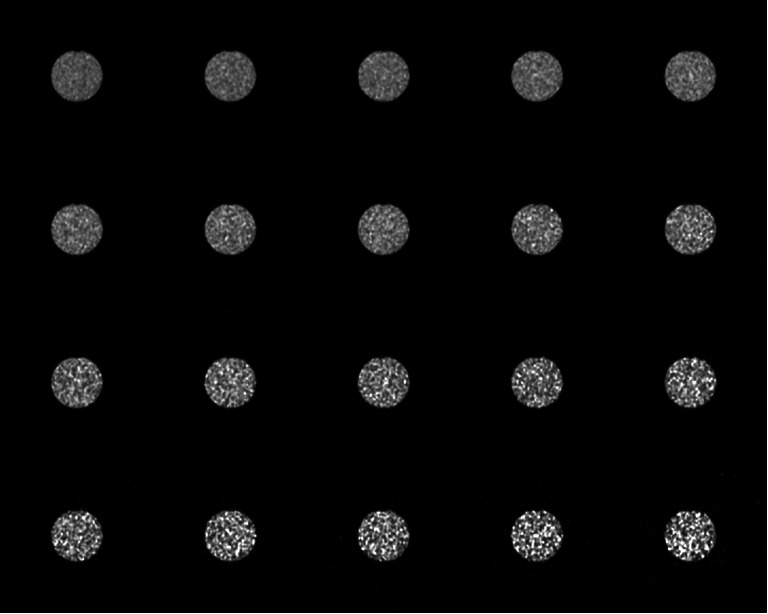
Slice 21 (all time frames, 1 to 20) reconstructed with RAMLA

Fig. 9.

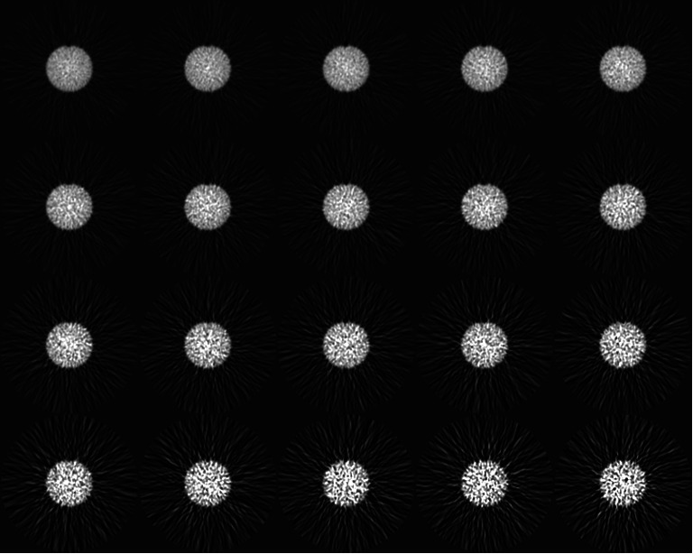
Slice 21 (all time frames, 1 to 20) reconstructed with FBP

Fig. 10.

3D case: STD/mean, kurtosis, and skewness with respect to experimental data. Cylindrical VOI was selected on images (slices 4 to 42) reconstructed with RAMLA (a through c) and FBP (d through f)

Table 4.

3D case (all time frames (1 to 20), VOI: slices 4 to 42), root mean square error (RMSE) for NSD, kurtosis, and skewness with respect to experimental data is compared between different models for data reconstructed with RAMLA and FBP

	Metric	NSD		Skewness		Excess kurtosis
	Reconstruction	RAMLA	FBP	RAMLA	FBP	RAMLA	FBP
Model	Poisson	0.2	0.3	0.5	0.5	0.7	2
	Negative binomial	0.003	0.03	2	8	12	117
	Normal	0.002	0.003	0.5	0.5	0.7	2
	Log-normal	0.003	0.1	0.9	1	3	6
	Gamma	0.003	0.03	0.1	0.3	0.4	1

Conclusions

This work presents an investigation of the statistical properties of noise in PET images reconstructed with filtered-backprojection and row-action maximum likelihood algorithm, after all clinical correction and image reconstruction procedures have been applied. This analysis has shown that the noise in PET images created with RAMLA reconstruction is very well characterized by gamma distribution followed closely by normal distribution, while FBP produces comparable conformity with both normal and gamma statistics. We have also shown that NSD (STD/mean) is modeled equally well by negative binomial, normal, log-normal, and gamma distributions for RAMLA and by negative binomial, normal, and gamma distributions for FBP reconstructions. While radioactive decay is well-modeled as a Poisson process, the net result after all correction and image reconstruction techniques have been applied is decidedly non-Poisson. This has important implications for an accurate evaluation of quantitative information provided by PET imaging. It is particularly true for dynamic PET imaging, where the signal to noise ratio decreases for each subsequent time frame, which can pose significant challenges for quantitative analysis. A large number of noise reduction techniques are predicated on additive noise models and an incorrect treatment of image noise can be detrimental to adequate algorithm performance. Noise reduction algorithms specifically designed for Poisson noise are expected to produce inferior results when applied to clinical PET images.

References

- 1.Caldwell CB, et al. Observer variation in contouring gross tumor volume in patients with poorly defined non-small-cell lung tumors on CT: The impact of 18FDG-hybrid PET fusion. Int J Radiat Oncol Biol Phys. 2001;51(4):923–931. doi: 10.1016/S0360-3016(01)01722-9. [DOI] [PubMed] [Google Scholar]
- 2.Sailer SL, et al. Improving treatment planning accuracy through multimodality imaging. Int J Radiat Oncol Biol Phys. 1996;35(1):117–124. doi: 10.1016/S0360-3016(96)85019-X. [DOI] [PubMed] [Google Scholar]
- 3.Bar-Shalom R, et al. Clinical performance of PET/CT in evaluation of cancer: Additional value for diagnostic imaging and patient management. J Nucl Med. 2003;44(8):1200–1209. [PubMed] [Google Scholar]
- 4.Bradley JD, et al. Implementing biologic target volumes in radiation treatment planning for non-small cell lung cancer. J Nucl Med. 2004;45(Suppl 1):96S–101S. [PubMed] [Google Scholar]
- 5.Drever LA: Positron emission tomography target volume delineation xiv + 134. Thesis, University of Alberta, 2005
- 6.Pieterman RM, et al. Preoperative staging of non-small-cell lung cancer with positron-emission tomography. N Engl J Med. 2000;343(4):254–261. doi: 10.1056/NEJM200007273430404. [DOI] [PubMed] [Google Scholar]
- 7.Kubota K, et al. Differential diagnosis of lung tumor with positron emission tomography: A prospective study. J Nucl Med. 1990;31(12):1927–1932. [PubMed] [Google Scholar]
- 8.Weber W, et al. Assessment of pulmonary lesions with 18F-fluorodeoxyglucose positron imaging using coincidence mode gamma cameras. J Nucl Med. 1999;40(4):574–578. [PubMed] [Google Scholar]
- 9.Vardi Y, Shepp LA, Kaufman L. A statistical model for positron emission tomography. J Amer Stat Assoc. 1985;80(389):8–20. doi: 10.1080/01621459.1985.10477119. [DOI] [Google Scholar]
- 10.Tsui BM, et al. Analysis of recorded image noise in nuclear medicine. Phys Med Biol. 1981;26(5):883–902. doi: 10.1088/0031-9155/26/5/008. [DOI] [PubMed] [Google Scholar]
- 11.Rzeszotarski MS. Counting statistics. Radiographics. 1999;19(3):765–782. doi: 10.1148/radiographics.19.3.g99ma33765. [DOI] [PubMed] [Google Scholar]
- 12.Rowe RW, Dai S. A pseudo-Poisson noise model for simulation of positron emission tomographic projection data. Med Phys. 1992;19(4):1113–1119. doi: 10.1118/1.596774. [DOI] [PubMed] [Google Scholar]
- 13.Lange K, Carson R. EM reconstruction algorithms for emission and transmission tomography. J Comput Assist Tomogr. 1984;8(2):306–316. [PubMed] [Google Scholar]
- 14.Shepp LA, Vardi Y. Maximum likelihood reconstruction for emission tomography. IEEE Trans Med Imag. 1982;1(2):113–122. doi: 10.1109/TMI.1982.4307558. [DOI] [PubMed] [Google Scholar]
- 15.Shepp LA, Logan BF. Fourier reconstruction of a head section. IEEE Trans Nucl Sci. 1974;NS21(3):21–43. [Google Scholar]
- 16.Kadrmas DJ. LOR-OSEM: Statistical PET reconstruction from raw line-of-response histograms. Phys Med Biol. 2004;49(20):4731–4744. doi: 10.1088/0031-9155/49/20/005. [DOI] [PMC free article] [PubMed] [Google Scholar]
- 17.Razifar P: Novel approaches for application of principal component analysis on dynamic pet images for improvement of image quality and clinical diagnosis. Digital Comprehensive Summaries of Uppsala Dissertations from the Faculty of Science and Technology, x + 89, 2005
- 18.Wahl RL. In: Principles and Practice of Positron Emission Tomography. Wahl RL, editor. Philadelphia: Lippincott Williams & Wilkins; 2002. p. 442. [Google Scholar]
- 19.Green GC: Wavelet-based denoising of cardiac PET data xiv + 135. Dissertation, Carleton University, 2005
- 20.Ollinger JM, Fessler JA. Positron-emission tomography. EEE Signal Process Mag. 1997;14(1):43–55. doi: 10.1109/79.560323. [DOI] [Google Scholar]
- 21.Coxson PG, Huesman RH, Borland L. Consequences of using a simplified kinetic model for dynamic PET data. J Nucl Med. 1997;38(4):660–667. [PubMed] [Google Scholar]
- 22.Slifstein M, Mawlawi OR, Laruelle M. Chapter 11 (816): Partial volume effect correction: Methodological considerations. In: Gjedde A, Hansen SB, Knudsen GM, Paulson OB, editors. Physiological Imaging of the Brain with PET. San Diego: Academic; 2000. p. 413. [Google Scholar]
- 23.Rodrigues I, Sanches J, Bioucas-Dias J: Denoising of medical images corrupted by poisson noise. 15th IEEE International Conference on Image Processing 1–5(ICIP 2008):1756–1759, 2008
- 24.Hannequin P, Mas J. Statistical and heuristic image noise extraction (SHINE): A new method for processing Poisson noise in scintigraphic images. Phys Med Biol. 2002;47(24):4329–4344. doi: 10.1088/0031-9155/47/24/302. [DOI] [PubMed] [Google Scholar]
- 25.Němeček P: Filtrace šumu ve scintigrafických snímcích metodou založenou na Correspondence Analysis. v + 47, 2006
- 26.Seret A, Vanhove C, Defrise M. Resolution improvement and noise reduction in human pinhole SPECT using a multi-ray approach and the SHINE method. Nuklearmedizin. 2009;48(4):159–165. doi: 10.3413/nukmed-0215. [DOI] [PubMed] [Google Scholar]
- 27.Budinger TF, et al. Quantitative potentials of dynamic emission computed tomography. J Nucl Med. 1978;19(3):309–315. [PubMed] [Google Scholar]
- 28.Browne J, de Pierro AB. A row-action alternative to the EM algorithm for maximizing likelihood in emission tomography. IEEE Trans Med Imag. 1996;15(5):687–699. doi: 10.1109/42.538946. [DOI] [PubMed] [Google Scholar]
- 29.Mandelkern MA. Nuclear techniques for medical imaging: Positron emission tomography. Annu Rev Nucl Part Sci. 1995;45:205–254. doi: 10.1146/annurev.ns.45.120195.001225. [DOI] [Google Scholar]
- 30.Wilson DW, Tsui BMW. Noise properties of filtered-backprojection and ML-EM reconstructed emission tomographic images. IEEE Trans Nucl Sci. 1993;40(4):1198–1203. doi: 10.1109/23.256736. [DOI] [Google Scholar]
- 31.Soares EJ, Byrne CL, Glick SJ. Noise characterization of block-iterative reconstruction algorithms: I. Theory. IEEE Trans Med Imaging. 2000;19(4):261–270. doi: 10.1109/42.848178. [DOI] [PubMed] [Google Scholar]
- 32.Tanaka E, Kudo H. Subset-dependent relaxation in block-iterative algorithms for image reconstruction in emission tomography. Phys Med Biol. 2003;48(10):1405–1422. doi: 10.1088/0031-9155/48/10/312. [DOI] [PubMed] [Google Scholar]
- 33.Dempster AP, Laird NM, Rubin DB. Maximum likelihood from incomplete data via the EM algorithm. J Roy Stat Soc B Meth. 1977;39(1):1–38. [Google Scholar]
- 34.Hudson HM, Larkin RS. Accelerated image reconstruction using ordered subsets of projection data. IEEE Trans Med Imaging. 1994;13(4):601–609. doi: 10.1109/42.363108. [DOI] [PubMed] [Google Scholar]
- 35.Gonzalez RC, Woods RE. In: Digital Image Processing. 3. Anonymous, editor. Upper Saddle River: Pearson Prentice Hall; 2008. p. 954. [Google Scholar]
- 36.NIST/SEMATECH: e-handbook of statistical methods. 2006(07/05/2006), 2010
- 37.Hilbe J. In: Negative Binomial Regression. Anonymous, editor. Cambridge: Cambridge University Press; 2007. p. 251. [Google Scholar]
- 38.Barrett HH, Wilson DW, Tsui BM. Noise properties of the EM algorithm: I. Theory. Phys Med Biol. 1994;39(5):833–846. doi: 10.1088/0031-9155/39/5/004. [DOI] [PubMed] [Google Scholar]