A Fully Automatic Method for Lung Parenchyma Segmentation and Repairing

Abstract

Considering that the traditional lung segmentation algorithms are not adaptive for the situations that most of the juxtapleural nodules, which are excluded as fat, and lung are not segmented perfectly. In this paper, several methods are comprehensively utilized including optimal iterative threshold, three-dimensional connectivity labeling, three-dimensional region growing for the initial segmentation of the lung parenchyma, based on improved chain code, and Bresenham algorithms to repair the lung parenchyma. The paper thus proposes a fully automatic method for lung parenchyma segmentation and repairing. Ninety-seven lung nodule thoracic computed tomography scans and 25 juxtapleural nodule scans are used to test the proposed method and compare with the most-cited rolling-ball method. Experimental results show that the algorithm can segment lung parenchyma region automatically and accurately. The sensitivity of juxtapleural nodule inclusion is 100 %, the segmentation accuracy of juxtapleural nodule regions is 98.6 %, segmentation accuracy of lung parenchyma is more than 95.2 %, and the average segmentation time is 0.67 s/frame. The algorithm can achieve good results for lung parenchyma segmentation and repairing in various cases that nodules/tumors adhere to lung wall.

Introduction

Lung cancer is one of the most serious cancers in the world. In fact, the total number of deaths caused by lung cancer is greater than the sum of breast, prostate, and colorectal cancers [1,2]. Early detection and treatment of lung cancer can improve the survival rate of the patients [3]. Computed tomography (CT) is an important instrument for early detection of nodules, but interpreting the large amount of thoracic CT images is a very challenging task for radiologists. Computer-aided detection/diagnosis (CAD) is considered as a promising tool to aid the radiologist in lung nodule CT interpretation.

In a lung CAD system, prior to the detection of lung lesions, the segmentation of lung parenchyma from thoracic images [4–6] has to be conducted in order to reduce the amount of computation to minimize the computation time. Good lung segmentation can improve the efficiency of the entire CAD system and reduce misdiagnosis. Therefore, the lung parenchyma segmentation is a key procedure of a CAD system for lung diseases and pulmonary function assessment [7], which will affect the accuracy of the whole lung CAD system.

In recent years, scholars from various countries have put forward a series of lung segmentation methods [8–15]. Typically, these methods can be generally divided into the following three categories: threshold method [16], region-growing method [17,18], and pattern classification method [19]. Threshold method is simple and fast, but it is unable to rule out the tracheal/bronchial area effectively and cannot include nodules attached to the lung parenchyma edge region. Region-growing method is semi-automatic segmentation algorithm. Although the method can segment high-density areas attached to the lung parenchyma edge, but it cannot separate the two lung lobes, it also needs to select manually a seed point. It is sensitive to the selection of parameters concerning rules of region growing and incorporating, which may affect the stability. Pattern classification method requires a large number of training sample data, and needs to extract the features, so the processing time is longer. It cannot meet the real-time requirements of the CAD system in clinical application.

For medical CT lung images, there is a kind of nodule/tumor which is adhered to a lung wall, i.e., juxtapleural nodule. It is important in the judgment of early-stage lung cancer/disease, we cannot afford to ignore it. However, due to the gray value is very similar to the fat outside the lung wall. In the lung parenchyma segmentation process, the juxtapleural nodule is often mistakenly judged as the fat to exclude. Therefore in the subsequent disease, diagnosis ignores impact of the lesion, and influences the diagnosis of the illness, reduces the accuracy of the diagnosis. The nodules/tumors are often mistaken as fat, and the corresponding region in the segmented lung parenchyma becomes a sunken area to the lung wall. Due to the importance of this kind of nodules/tumor in diagnosis, many scholars are trying to take measures to improve the method. The “the rolling-ball” method [18] is one of the most commonly used one. However, the “the rolling-ball” cannot accurately judge the size of the defect, so it is difficult to set the sphere radius accurately.

Considering the problems above in lung segmentation, this paper presents a fully automatic algorithm for lung parenchyma segmentation and repairing. First, optimal iterative threshold method is adopted for binarization. Then, three-dimensional (3-D) connectivity labeling and 3-D region growing are utilized to remove the main trachea. Two lung lobes are judged to see whether they are connected. If connected, center position locating method is used to separate of left lung from the right. Finally, the original segmented lung parenchyma will be repaired based on an improved chain code method and Bresenham algorithm. The whole process of the algorithm is depicted in Fig. 1. Lung segmentation algorithm proposed in this paper can effectively reduce the missing of juxtapleural nodules, and the method makes a full use of 3-D CT image sequence. The segmentation accuracy and implementation speed have been improved greatly than the rolling-ball method.

Fig. 1.

Flow chart of automatic lung parenchyma segmentation and repairing based on improved chain code and Bresenham

Methods

A schematic of the different stages of our method is given in Fig. 1. The proposed algorithm can be divided into two stages: (1) initial segmentation of lung parenchyma based on sequent images and (2) lung parenchyma repairing based on improved chain code and Bresenham algorithm. Each stage comprises different substages. The details are given below. After the description of lung parenchyma segmentation and repairing methods, evaluation methods are introduced in this section.

Initial Segmentation of Lung Parenchyma Based on Sequential Images

Original thoracic CT images include the examination bed, fat, ribs, lung parenchyma, main trachea, etc. as are shown in Fig. 2. Pulmonary lesions are within the lung parenchyma. Before the detection of pulmonary disease, tissues outside the lung parenchyma should be removed, and the whole lung parenchyma should be segmented from the original thoracic CT images, in order to reduce the amount of computation, to speed up the process of implementation, and to minimize the interference of regions outside lung parenchyma. Initial segmentation of the lung parenchyma is to remove tissues outside of the lung parenchyma from the original image.

Fig. 2.

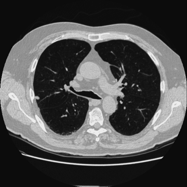
An original thoracic CT image

Initial Segmentation of Lung Parenchyma Area

Lung parenchyma is filled with air and its density is relative low. It can be separated from the ribs and the surrounding tissues such as fat due to the densities are different. In CT images, the HU value reflects the corresponding density and forms its gray value in CT images. For the same machine, the HU values of lung parenchyma in CT images are almost the same for different patients. In this paper, the optimal threshold value is obtained through an iterative procedure to segment lung parenchyma regions initially. The process is as follows:

1. Set the initial background gray-scale F_b, object grayscale F₀, the initial threshold value is .

2. Calculate the average gray level of the background region and object region G_b and G₀.

3. Set , and the new threshold is T₁.

4. Iteration termination condition is T₁≈T₀, that is, the difference between T₁ and T₀ is less than 5. Otherwise assign T₁ values to T₀, and go back to step (2)

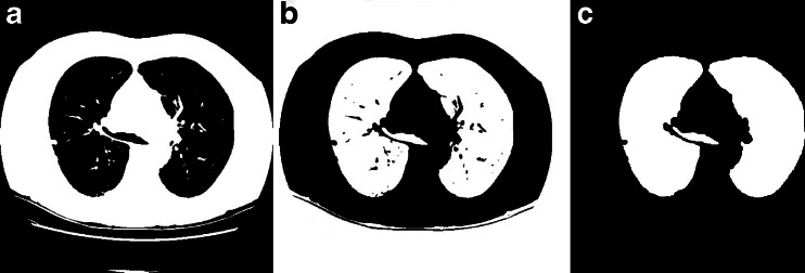
The above process will converge after 6 to 12 times of iteration, in the obtained binary image (as shown in Fig. 3a). The region outside the body and lung parenchyma region is black.

Fig. 3.

Initial segmentation of lung parenchyma. a Binarized image by iterative threshold. b Inverted image. c Initial mask after removing background

3-D Connected Component Labeling to Remove the Background

After iterative threshold processing, the background and the low gray pixels are labeled black; fat and tissues outside lung parenchyma are labeled white, as shown in Fig. 3a. Then make the image inverted, and label 3-D connecting components on the binary images. All the background pixels connected with the lung boundaries are negated, and the results are as shown in Fig. 3b. After the above steps to deal with image sequences, only the lung (white), trachea, bronchus (white), and vascular, nodular black hole, some residual background (white) are left, as shown in Fig. 3c.

3-D Region-Growing Method to Remove the Main Trachea

After these two steps of processing, main trachea, and bronchus are usually preserved, as shown in Fig. 4a. Lung trachea and bronchus can be easily removed if the trachea is not close to the lung in the steps of “3-D Connected Component Labeling to Remove the Background.” However, when the lobar bronchi enter the lungs or are connected with the lung [20], they will be marked as lung area in the process of connecting component labeling. According to the anatomy knowledge, air is filling trachea, and CT value of air in the CT image is in a fixed range. Therefore, this paper adopts an improved 3-D region-growing method to remove the trachea and the bronchus. In the 3-D region-growing method, selection of seed points, rules of region growing and terminating, are described as follows:

1. Selection of seed points

   From anatomical knowledge, in a CT scan, the trachea appears as early as the apex. Therefore, the computation starts to find a connected domain of the specified size from the first slice of the sequences and select the centroid of the target area (trachea) as the initial seed point. Seed points are identified in subsequent CT sections based on the centroid location of the segmented trachea region in the previous section [18].

2. Rules of region growing

   In our algorithm, 3-D region-growing conditions are defined according to the CT values of the organizations by the similarity criteria [20]. We define a variable: the maximum gray-level threshold d. Compare the current point grayscale with average grayscale of all pixels in the segmented area. When the difference is less than or equal to d, the pixel is added to the segmented area.

3. Terminating region growth

   For a single slice image, when the absolute difference of the pixel gray value and average gray of the segmented region is less than or equal to d, the region growing stops. For a sequence of images, when tracheal area after the (i)th time growing minus the tracheal area of (i-1)th time, and the difference is less than a certain area, the growing ends. That is, a stopping criterion is established to halt the region-growing process when the trachea has been adequately segmented. This stopping criterion is satisfied when the area of the trachea at iteration i is less than 5 pixels greater than the corresponding area at iteration i-1 [18].

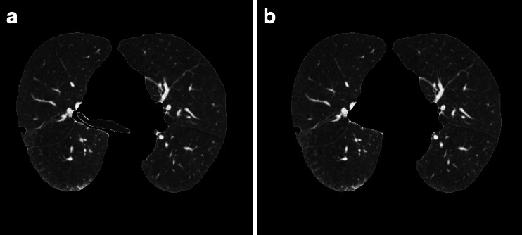
   The experimental result is as is illustrated in Fig. 4a. Wherever the trachea and the lung are connected or separated, our algorithm can split the main trachea and bronchus accurately, as is shown in Fig. 4b.

Fig. 4.

Removal of the main trachea adhered with lung parenchyma. a Initial segmented lung parenchyma. b Removing the main trachea

Separation of Left and Right Lungs

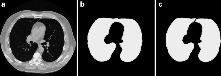
After removing the trachea, if left and right lungs are sticking together, as is depicted in Fig. 5a, b, lung separation must be carried out, to be ready for lung nodule CAD or pulmonary function assessment. This paper presents a simple and effective algorithm for left and right lung separation, that is, center location method.

Fig. 5.

Separation of the two lung lobes. a Original thoracic CT image. b Initial segmented mask (two lobes are connected). c Separated two lobes

Separation of left and right lung is mainly related to three issues: how to determine whether the left and the right lungs are adhered; how to quickly locate the area of the adherence; and how to separate the left and the right lungs. Here, the separation steps of left and right lung are designed as follows:

1. The judgment about the adherence of left and right lungs is based on the connecting domain. In images of removing trachea, bronchus, fat and other tissues, there should be only two identifiable larger connectivity lung regions. Other parts of the connected domain will be much smaller. If there is only one connectivity region, the two lung lobes can be thought as connected. In addition, if there is one more connectivity region, and area ratio between the first and the second largest region is over a threshold T, then the two lung lobes can be thought of as connected, and this threshold T is set as an empirical value 9.

2. Calculate the width and the height of the binarized lung parenchyma region respectively, and then calculate the center of the lung parenchyma region p (m, n).

3. Scan the binary image, the scanning region is: row range from row m to the height of the image, column range of n − 30 to n + 30, get the point with the least white pixels, and denoted by q(x, y), get region of (x − 30, x + 30), (y − 30, y + 30) as region of interest.

4. For the above identified region of interest-segmented mask images, process as follows:

   1. Scanning the ith row, if there are three black pixels in the row, then the first and last black pixels are denoted by A_i and B_i and get the midpoint C_i of A_i and B_i. If there are no black pixels, or more than three black pixels, no midpoint will be obtained;
   2. Link up C₁, C₂, …,C_i as the dividing line, then do morphological erosion to the mask image along the dividing line with a structure element of black ball whose radius is 1.

The processing result is depicted as Fig. 5c. Our algorithm can separate two lung lobes accurately.

Lung Parenchyma Repairing Based on the Improved Chain Code and Bresenham Algorithm

Lung parenchyma can be segmented from original thoracic CT image as is described in “Initial Segmentation of Lung Parenchyma Based on Sequential Images.” But if there are nodules or tumors adhered to the lung wall, they will be wiped off as fat or other tissues, and it will form a concave region on the corresponding lung border. This will bring miss diagnosis because they are important for lung disease CAD system. In this paper, we propose a lung parenchyma repairing method based on the improved chain code and Bresenham algorithm, to avoid the missing of nodules or tumors adhered to the lung wall.

Discrimination of Concavity and Convexity of Boundary Points Based on Chain Code Difference

Chain code is used to represent a boundary through a specified length and a direction of straight section by a serial number [21,22]. Suppose there are N points on the boundary, for each point on the boundary there is a chain code A(i) which points to this point from a pre-point and a chain code A(i + 1) which points to the next point from this point. The so-called relative chain code is the relationship between A(i) and A(i + 1). If they are in the same direction, the relative chain code is zero. Absolute chain code is the accumulated value of the relative chains from the starting point. The absolute chain code of the starting point can be set to zero. Its absolute value will increase by 8 after moving along the border one circle.

The sum of three-point chain code is the sum of absolute chain codes of the current point A(i) and the forehead two points A(i − 1), A(i − 2), that is

1

Chain code difference means the difference between Sum(i + 3) and Sum(i), that is

2

Chain code difference means the difference between the two directions and is proportional to the amount of curvature. When the boundary points are calculated in the clockwise direction, a point will be concave if the difference is positive. Otherwise, it will be convex.

According to every point’s chain code difference of the boundary, we can draw the chain code difference curve corresponding to the boundary. Thus, we can distinguish the boundary’s concavity and convexity through the chain code difference curve. The algorithm to distinguish the boundary’s concavity and convexity through the chain code difference can be summarized as follows:

1. Binarize the image, find its boundary.

2. Determine the starting point of chain code and write down the location of the point. Here, the nearest boundary point from the top left corner is as the starting point.

3. Determine the chain code’s direction of rotation clockwise or counterclockwise.

4. Calculate every point’s chain code difference Diff(i) of the boundary.

5. Set a threshold according to the characteristics of the chain code difference. Then, distinguish every point’s concavity and convexity. In this paper, the point is convex when Diff(i) < −1, the point is concave when Diff(i) > 2.

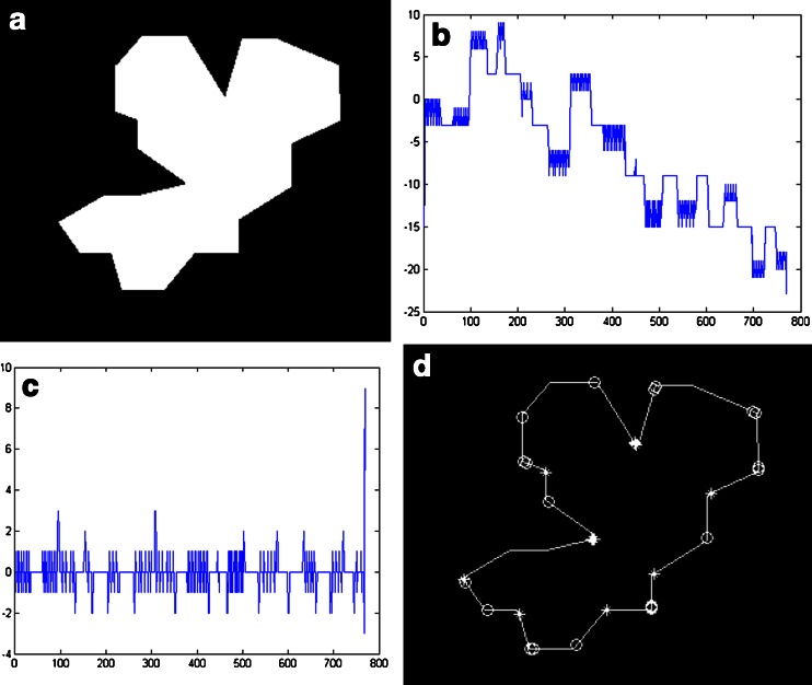
Here, we use an image that contains a variety of convex–concave points to verify the algorithm. Figure 6 shows the calculated results of chain code values and the marked convex–concave points. Figure 6a is the original image; Fig. 6b shows the sum of three-point chain code; Fig. 6c shows the difference of three-point chain code; Fig. 6d shows the marked convex–concave points. In Fig. 6d, “o” indicates convex point, and “*” indicates concave point.

Fig. 6.

The value of chain code and discrimination of convex–concave points

In Fig. 6c, we can find there are eight places where their values are greater than 2 and thirteen places where their values are less than −1. Referring to the threshold of the literature [23], the point is convex when Diff(i) < −1, the point is concave when Diff(i) > 2, and the marked convex–concave points are shown in Fig. 6d after judging. We can see the algorithm’s judgment and the markers of convex–concave points are very accurate.

Repair the Sunken Boundary According to Convex–Concave Points

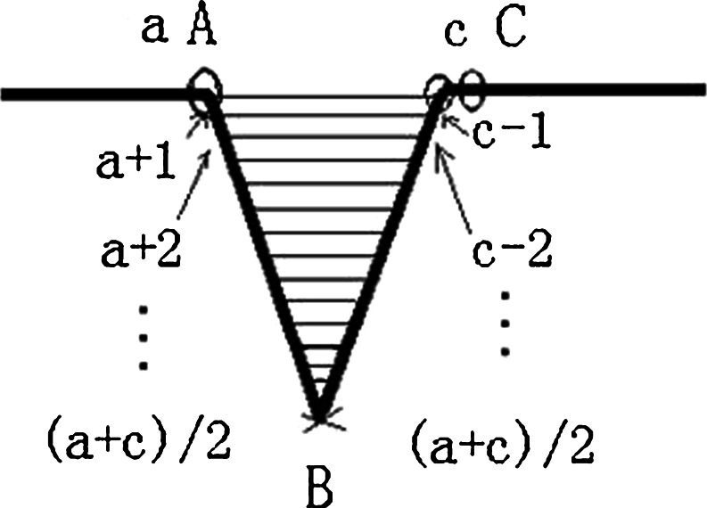
After distinguishing every point’s concavity and convexity of the boundary, repair the sunken boundary according to these points’ concavity and convexity. To illustrate the repairing process, we amplify part of the Fig. 5d, as is illustrated in Fig. 7. The steps of boundary repairing according to concavity and convexity are summarized as follows:

1. Set the loop, look for convex points, update convex point A, and write down its coordinate (x1, y1) and its position a in the chain code, which is the location of the point relative to the starting point in the boundary.

2. Pause when encountering a concave point B. Write down its coordinate (x2, y2) and its position b in the chain code.

3. Continue to search along the direction of the chain code until to find the nearest convex point C from the point B. Then, write down the convex point C’s coordinate (x3, y3) and its position c in the chain code.

4. If the point after point C is also a convex point, then update the point C. Write down the updated point’s coordinate (x3, y3) and its position c.

5. Connect the convex point A and the convex point C.

6. Find the filling border in the radian domain formed by line AC and the boundary. That is to connect the boundary’s points a + 1 (which is the next point of point a on the boundary) and c − 1 (which is the former point of point c on the boundary), a + 2 and c − 2, a + 3 and c − 3 …until the point (a + c)/2 in turn.

Fig. 7.

The illustration of filling

Using Bresenham Algorithm to Fill the Sunken Boundary

Bresenham proposed the famous two-dimensional linear space generated method [24]. In this paper, we use the Bresenham algorithm to fill the boundary sunken area of the lung parenchyma. The basic idea is two endpoints’ coordinates of a known straight line are A(x₁, y₁) and B(x₂, y₂).

Assume that the slope of the straight line between 0 and 1, order

3

Then the slop k is:

4

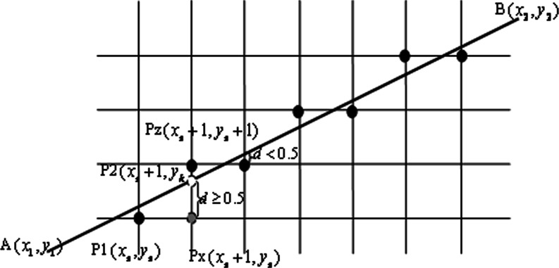
As Fig. 8 has shown, P1 (x_s, y_s) is the closest pixel to the starting point A of the straight line, if x coordinates increase 1, the y coordinate should increase k, and reach the point of P2 (x_s + 1, y_k). The next point of P1 in the right direction is Px, with coordinates (x_s + 1, y_s), and the next point of the top right is Pz with coordinates (x_s + 1, y_k + 1).

Fig. 8.

Principle illustration of Bresenham algorithm

Set the grid unit to 1, one pixel distance. If the distance between P2 and Px is no less than half a unit, that is, the distance d ≥ 0.5, then take the next point of P1, which is Pz, with coordinates (x_s + 1, y_s + 1). Otherwise, if the distance between P2 and Px is less than half a unit, that is, the distance d < 0.5, then take the next point of P1, which is Px, with coordinates (x_s + 1, y_s). It can be described as:

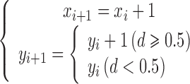5

Here, the key issue is the error term d. The initial value is 0, for every step d = d + k. Whenever there is an increase of 1 at the y direction, it will move forward a step, and d subtract 1, that is d = d − 1.

For simplicity, take e = d − 0.5, and Eq. (5) changes to

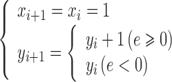6

Here, the initial value of e is −0.5, for every step e = e + k. Also, whenever there is an increase of 1 at the y direction, it will move forward a step, and e subtract 1, that is .

All of the discussion above is a simple case with slope between 0 and 1. As for the general condition, the followings should be conducted:

1. When the absolute value of slope is greater than 1.0, exchange x and y, dx and dy.

2. Increase or reduce 1 to control x (or y) according to the sign of dx (or dy).

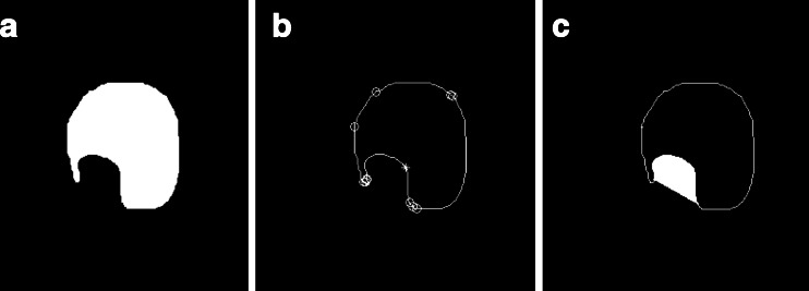
In order to test the accuracy of the filling algorithm, different structures of graphics and lung parenchyma images are used for verification respectively. The results of filling of Fig. 6a are shown in Fig. 9. Another image shown in Fig. 10a is used to experiment, in which there is a nonrigid concave area. Convex–concave points are marked in Fig. 10b; the filling result is shown in Fig. 10c. Here, we can see whether the concave region is rigid or not. All of the filling results are satisfactory by our repairing algorithm. For the lung parenchyma boundary filling example of Fig. 2, with the right lung wall nodules case, the repairing process is illustrated in Fig. 11. Figure 11a depicts the mask of initial segmentation; Fig. 11b shows labeling of convex–concave points on the boundary, where “+” indicates convex point and “o” indicates concave point; Fig. 11c shows the filling areas by Bresenham algorithm; Fig. 11d shows the obtained mask after repairing; and Fig. 11e shows the final segmentation results.

Fig. 9.

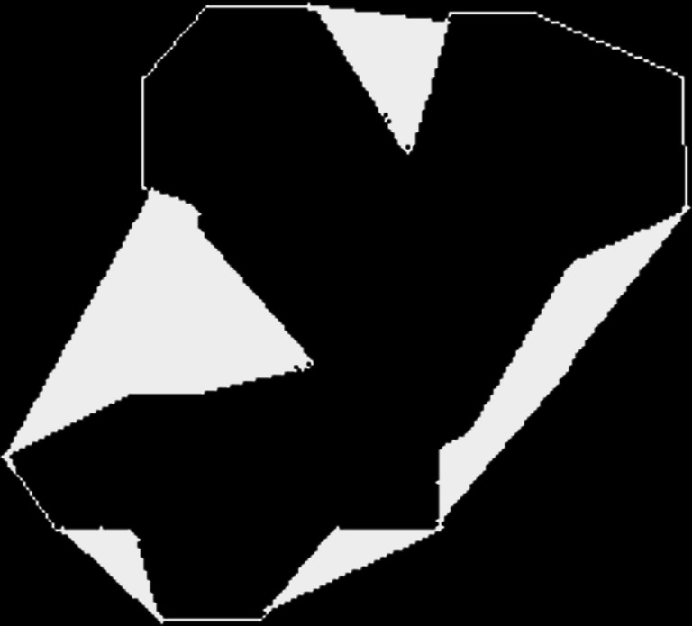
Image of filling result for Fig. 6a

Fig. 10.

Another example for filling

Fig. 11.

An example for lung parenchyma repairing

Evaluation Methods

The segmentations from the automated algorithms have been compared with manual segmentations. Manual contours were traced by three experienced chest radiologists on all slices from the top to bottom parts of the lungs. The manual segmentation results were judged consensually by the panel and are used as the golden standard, with which the performance of automated algorithms was compared. Quantitative measures for segmentation accuracy are applied according to the following metrics.

Segmentation Accuracy of the Whole Lung Parenchyma

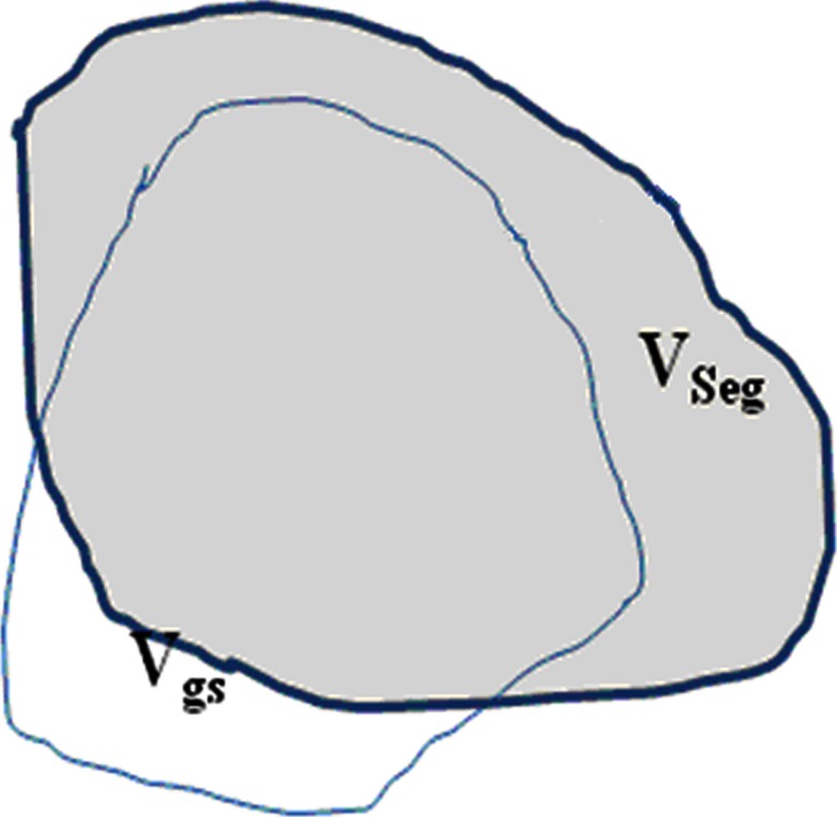
In order to quantitatively evaluate the segmentation accuracy, here we use the overlapping areas between the segmentation results and the golden standard, to measure the degree of coincidence as segmentation accuracy. Figure 12 shows the illustration of segmentation accuracy, in which, V_Seg, is segmented area of lung parenchyma area (number of pixels) which is obtained automatically by segmentation algorithm, while V_gs is the golden standard area (number of pixels).

Fig. 12.

The illustration of segmentation accuracy

Overlap as the accuracy of lung segmentation is defined as:

7

Overlap can effectively describe the difference between segmented lung parenchyma region and golden standard. Overlap values are in the range of 0~100 %. When the automatic segmentation and manual segmentation results are in agreement, V_Seg and V_gs overlap completely, and the overlap value will be the maximum, of 100 %, which means the automatic segmentation method will achieve the most ideal results; otherwise, if there is greater difference between automatic segmentation and manual segmentation results, that is, V_Seg and V_gs have smaller overlapped region, the value of overlap will be smaller, and the automatic segmentation will have less satisfactory results.

Accuracy of Including Juxtapleural Nodule Regions

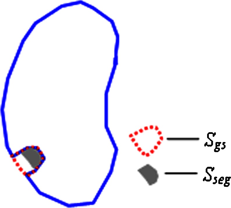
We define a metrics of including_accuracy to measure the accuracy of including juxtapleural nodule regions as is illustrated in Fig. 13. S_Seg is segmented area of juxtapleural nodule (number of pixels) that is obtained automatically by segmentation algorithm, while S_gs is the golden standard area (number of pixels). The including_accuracy is defined as:

8

Fig. 13.

The illustration of including accuracy of juxtapleural nodules

The including_accuracy ranges from zero (not including the juxtapleural nodules) to 100 % (totally including the juxtapleural nodules).

Experiments and Results

Databases

A Lung Nodule Database and a Juxtapleural Nodule Database Are Set to Evaluate the Effectiveness of the Proposed Method

The Lung Nodule Database includes 97 thoracic CT scans, they are from ShengJing Hospital affiliated to Chinese Medical University and Beijing Xuanwu Hospital of China. The samples were collected retrospectively from 97 patients with 66 males and 31 females; age range from 37 to 82, with an average age of 62.3. The slice thickness is from 0.75 to 5 mm, and the total slice number of each scan varies from 129 to 395 with an average of 195/scan. The X-ray tube current ranges from 30 to 220 mA. Of those 97 scans, 67 scans have 30 mA tube current, 10 scans at 50 mA, and the other 20 scans are above 100 mA. The pixel dimensions range from 0.51 to 0.74 mm, the pixel matrices are 512 × 512. There are 197 nodules in the dataset; the nodule diameter range is 4–30 mm, with an average of 19 mm; the CT value range is 20–50 HU.

The Juxtapleural Nodule Database includes 25 thoracic CT scans, which are from the same hospitals. Of the 25 patients, there are 16 males and 7 females; the age range is 43–77 years old, with an average of 59.4 years old. The acquisition parameters are the same as abovementioned. Among the 25 scans, 16 scans are at 30 mA tube current with 2-mm slice thickness, 7 scans at 50 mA with 5-mm slice thickness, and the other 2 scans are 120 mA with 5-mm slice thickness. There is at least one juxtapleural nodule in each scan, with a total of 32 juxtapleural nodules in the dataset. The nodule diameter ranges from 8 to 25 mm, with an average of 16 mm; the CT value range is 25–40 HU, with an average of 30 HU; 16 juxtapleural nodules are subtle GGO which are in the scans at 30 mA tube current.

Qualitative Results of Lung Parenchyma Segmentation and Repairing

Segmentation Process and Results

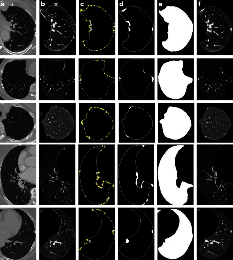
The proposed method can segment completely automatically and repair lung parenchyma properly. In the two datasets of 97 thoracic CT scans of lung nodule and 25 scans of juxtapleural nodule. By our algorithm of lung parenchyma segmentation and repairing, all the images have fine results of lung parenchyma segmentation and repairing, and all the 32 juxtapleural nodules are included well. Figure 14 illustrates the repairing process and the results of five images. Column (a) shows the original images, column (b) shows the initial lunge parenchyma segmentation results, column (c) shows labeling of convex–concave points on the boundary, column (d) shows filling areas by Bresenham algorithm, column (e) shows segmentation masks after repairing, and column (f) shows the final segmentation results.

Fig. 14.

Experiment results of lung parenchyma segmentation and repairing

Segmentation Results Compared with the Rolling-Ball Method

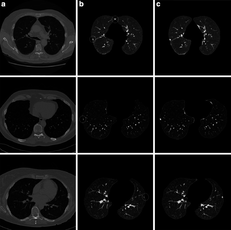
We compare our method with the most-cited rolling-ball method [17] to segment and repair lung parenchyma with juxtapleural nodule database. Here, the rolling-ball is 17 × 17 round structure element, and three of the segmentation results are shown in Fig. 15. In Fig. 15, column (a) shows the original image, column (b) shows the lunge parenchyma segmentation results by method of the rolling-ball, and column (c) shows the lung parenchyma segmentation results by our method. As we can see, in the first row, the rolling-ball method makes the two lung lobes linked together and misses the juxtapleural nodule partly; for the second and third rows, the juxtapleural nodules are both lost partly by the rolling-ball method. Whereas, all the three the lung parenchyma are segmented correctly by our method.

Fig. 15.

Comparison of segmentation results between the rolling-ball method and our algorithm

Quantitative Results of Segmentation Accuracy

We evaluate the quantitative results for the two databases, respectively. For the Lung Nodule Database, the segmentation accuracy of the whole lung parenchyma of the 97 CT scans was calculated. For the Juxtapleural Nodule Database, besides the segmentation accuracy of the whole lung parenchyma of the 25 CT scans, the accuracy of including juxtapleural nodule regions for the 32 juxtapleural nodules was also calculated.

Segmentation Accuracy for the Lung Nodule Database

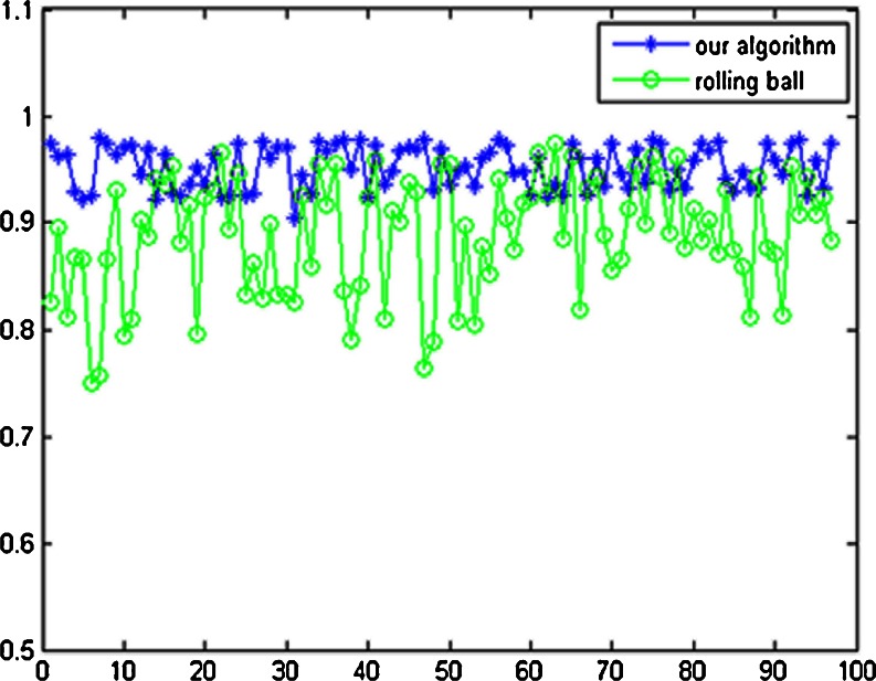
For the 97 CT scans of the Lung Nodule Database, segmentation accuracy (overlap) of the whole lung parenchyma is calculated by Eq. (7).The average overlap value of our algorithm is 95.24 %, with the standard deviation of 2.01 %; the average overlap value of the rolling-ball method is 88.82 %, with the standard deviation of 5.51 %. All the segmentation results by our automatic method are satisfactory, except for some tiny difference at lung border compared with manual-segmentation. For the 97 thoracic CT scans, the calculated results of overlap by our algorithm and the rolling-ball method are shown in Fig. 16.

Fig. 16.

Comparison of overlap value between the rolling-ball method and our algorithm

Segmentation Accuracy for the Juxtapleural Nodule Database

For the 25 CT scans of the Juxtapleural Nodule Database, overlap of 25 lung parenchyma and including_accuracy of 32 juxtapleural nodules are calculated by Eqs. (7) and (8), respectively. The average value of overlap and including_accuracy by our method and the rolling-ball method is given in Table 1. From the comparison, we can see that our method have much better performances for the processing of juxtapleural nodule cases.

Table 1.

Comparison results of our algorithm and the rolling-ball method

	Average of overlap (%)	Average of including_accuracy (%)
The rolling-ball method	88.82	45.34
Our algorithm	95.24	98.67

The comparison results show that our algorithm can better adapt various cases of the lung parenchyma segmentation than the rolling-ball method and achieve satisfactory segmentation results. From these experimental results, we can see that stable and satisfactory segmentation lung parenchyma results can be obtained automatically by the algorithm proposed in this paper.

Discussion

Analysis of Segmentation Error

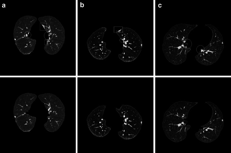
By our method, all of the experimented juxtapleural nodules are included well. The sensitivity of including juxtapleural nodules is 100 %, and the including_accuracy is 98.6 %, but the segmentation accuracy (overlap) of the whole lung parenchyma is approximately 96 %. This indicates that the main segmentation errors with our method do not occur in the position of juxtapleural nodules, but in other parts of lung parenchyma, which will not influence the proper diagnosis. Figure 17 shows three examples of segmentation errors occur compared with referenced standard, where three images in the first row are three segmentation results by our method, another three images in the second row are the corresponding referenced standard obtained as is described in “Evaluation Methods”. In Fig. 17, white circles and rectangles indicate the main segmentation errors compared with the corresponding referenced standard.

Fig. 17.

Three examples of segmentation results compared with referenced standard

For all the experiment of dataset of 122 thoracic CT scans (97 scans of the Lung Nodule Database and 25 scans of the Juxtapleural Nodule Database), the two main segmentation errors occur at lung hilar regions (which are marked with white circles in Fig. 17) and pleural sunken areas (which are marked with white rectangles in Fig. 17), which account for more than 95 % of the total segmentation errors.

Analysis of Computation Complexity

In the proposed lung parenchyma repairing method, the main computation is taken on the chain code and Bresenham algorithm. Suppose there are N points on the boundary, the chain code algorithm need N times of comparison operations. For one time of lung parenchyma repairing, as Fig. 7 illustrates, set , , and are coordinates of the three points A, B, and C; the filling needs times of adding operations, so the computational complexity of the proposed algorithm is , where X is distance between A and B, and k is times of parenchyma filling operations. Generally, in the process of lung parenchyma segmentation and repairing, k is less than 10. Obviously, in the worst cases the complexity is .

For the rolling-ball repairing method, if the radius of a rolling-ball is r pixels, the size of the structural element usually is pixels and it is scanned across the image. The computational complexity of the algorithm [12] will be , where the size of the image is .

We compare the implementation time of the proposed algorithm with the rolling-ball method. The configuration of the computer used for experiments is with Intel Core Duo 3.33 GHz CPU, RAM Memory 2 GB; the algorithms are used MatLab2010b programming. The comparison of implementation time between our algorithm and the rolling-ball method is given in Table 2, from which we can see that the average speed of our method is faster obviously than that of the rolling-ball method.

Table 2.

Comparison of implementation speed between our algorithm and the rolling-ball method

	The rolling-ball method	Our algorithm
Average speed/frame (s)	0.82	0.67

The analysis of computation complexity and comparison of implementation speed for lung parenchyma segmentation and repairing shows that our method is more efficient than the rolling-ball method.

Conclusions

In this paper, we comprehensively use several methods including optimal iterative threshold, 3-D connectivity labeling, 3-D region growing for the initial segmentation of the lung parenchyma, the method based on improved chain code and Bresenham algorithm to repair the lung parenchyma, and proposed a new automatic method for lung parenchyma segmentation and repairing.

Ninety-seven lung nodule thoracic CT scans and 25 juxtapleural nodule scans were used for experiments, and the proposed algorithm provides satisfactory performance and segmentation quality, with more than 95.2 % of segmentation accuracy of lung parenchyma, 98.6 % of the segmentation accuracy of juxtapleural nodule regions, and 100 % of juxtapleural nodule inclusion sensitivity. Compared with the most-cited rolling-ball method, our method shows such advantages as low computational cost, good performance of including juxtapleural nodules, easy implementation, and no user interaction.

The proposed method can meet the requirements of lung nodule CAD system, and provide high-quality pre-data for the sequential processing. The robustness of this approach in terms of other types of lung disease such as mesothelioma and emphysema, etc., remains to be verified further.

References

- 1.Rubin GD, Lyo JK, Paik DS, et al. Pulmonary nodules on multi-detector row CT scans: performance comparison of radiologists and computer-aided detection. Radiology. 2005;234(10):274–283. doi: 10.1148/radiol.2341040589. [DOI] [PubMed] [Google Scholar]
- 2.Bram VG, Bart MH, Max A. Computer-aided diagnosis in chest radiography. IEEE Trans Med Imaging. 2001;20(12):1228–1241. doi: 10.1109/42.974918. [DOI] [PubMed] [Google Scholar]
- 3.Lin DT, Yan CR, Chen WT. Autonomous detection of pulmonary nodules on CT image with a neural network-based fuzzy system. Comput Med Imag Graph. 2005;29(6):447–458. doi: 10.1016/j.compmedimag.2005.04.001. [DOI] [PubMed] [Google Scholar]
- 4.Qiang L. Recent progress in computer-aided diagnosis of lung nodules on thin-section CT. Comput Med Imag Graph. 2007;31(3):248–257. doi: 10.1016/j.compmedimag.2007.02.005. [DOI] [PMC free article] [PubMed] [Google Scholar]
- 5.Lee Y, Hara T, Fujita H, et al. Automated detection of pulmonary nodules in helical ct images based on an improved template-matching technique. IEEE Trans Med Imag. 2001;20(7):595–604. doi: 10.1109/42.932744. [DOI] [PubMed] [Google Scholar]
- 6.Farag A., El-Baz A., Gimelfarb G. G., Falk R., Hushek S. G. (2004) Automatic detection and recognition of lung abnormalities in helical CT images using deformable templates. Lecture Notes in Computer Science, Medical Image Computing and Computer-Assisted Intervention, 3217. Springer, New York, pp. 856–864
- 7.Hu S, Hoffman EA, Joseph MR. Automatic pulmonary segmentation for accurate quantitation of volumetric X-ray CT images. IEEE Trans Med Imag. 2001;20(6):490–498. doi: 10.1109/42.929615. [DOI] [PubMed] [Google Scholar]
- 8.Bian XY, Wu Y. A method of careful lung segmentation based on CT images. Journal of Chongqing University of Posts and Telecommunications (Natural Science Edition) 2010;22(5):665–668. [Google Scholar]
- 9.Armato SG, III, Giger ML, Moran CJ, et al. Computerized detection of pulmonary nodules on CT scan. RadioGraphics. 2000;19(5):1303–1311. doi: 10.1148/radiographics.19.5.g99se181303. [DOI] [PubMed] [Google Scholar]
- 10.Cuevas LM, Spieth PM, Carvalho AR, et al. Automatic lung segmentation of helical CT scans in experimental induced lung injury. IFMBE Proceedings. 2008;22:764–767. doi: 10.1007/978-3-540-89208-3_183. [DOI] [Google Scholar]
- 11.Guo SW, Zeng QS, Chen J. Extraction of pulmonary parenchyma in thoracic CT and computer aided diagnosis. Chin J Biomed Eng. 2008;27(5):788–791. [Google Scholar]
- 12.Pu JT, Justus R, Chin A, et al. Adaptive border marching algorithm: automatic lung segmentation on chest CT images. Comput Med Imag Graph. 2008;32:452–462. doi: 10.1016/j.compmedimag.2008.04.005. [DOI] [PMC free article] [PubMed] [Google Scholar]
- 13.Yuan KH, Xiang LX. Automated lung segmentation for chest CT images used for computer aided diagnostics. Journal of Tsinghua University. 2011;51(1):90–95. [Google Scholar]
- 14.Zhou YY, Feng HQ, Li CF. Automated lung segmentation in serial thoracic high resolution CT images. Beijing Biomedical Engineering. 2008;27(1):6–10. [Google Scholar]
- 15.Giorgio DN, Eleonora T, Antonella A, et al. Automatic lung segmentation in CT images with accurate handling of the hilar region. J Digit Imag. 2011;24(1):11–27. doi: 10.1007/s10278-009-9229-1. [DOI] [PMC free article] [PubMed] [Google Scholar]
- 16.Leader JK, Zheng B, Rogers RM. Automated lung segmentation in X-ray computed tomography: development and evaluation of a heuristic threshold-based scheme. Acad Radiol. 2003;10(11):1224–1236. doi: 10.1016/S1076-6332(03)00380-5. [DOI] [PubMed] [Google Scholar]
- 17.Hedlund LW, Anderson RF, Goulding PL. Two methods for isolating the lung area of a CT scan for density information. Radiology. 1982;144(2):353–357. doi: 10.1148/radiology.144.2.7089289. [DOI] [PubMed] [Google Scholar]
- 18.Armato SG, III, Sensakovic WF. Automated lung segmentation for thoracic CT impact on computer-aided diagnosis. Acad Radiol. 2004;11(9):1011–1021. doi: 10.1016/j.acra.2004.06.005. [DOI] [PubMed] [Google Scholar]
- 19.McNitt-Grag MF, Sayre JW, Huang HK, et al. Pattern classification approach to segmentation of digital chest radiographs and chest CT image slices. Proc SPIE. 1994;2167:465–476. doi: 10.1117/12.175080. [DOI] [Google Scholar]
- 20.Bai SL, Ying DJ. The anatomy. Beijing: People’s Health Publishing House; 2006. [Google Scholar]
- 21.Gonzalez RC, Richard EW, Steven LE (2004) Digital image processing using MATLAB[M]. Pearson Education, Inc., publishing as Prentice Hall, Englewood Cliffs
- 22.Lu ZQ, Tong T. The application of chain code sum in the edge form analysis [J] Int J Image Graph. 2002;7(12):1323–1328. [Google Scholar]
- 23.Tan JH, Zhang J. Identifying for the convex–concave of peripherals based on chain code difference. Science Technology and Engineering. 2007;7(5):769–772. [Google Scholar]
- 24.Tang ZS. Computer graphics algorithms. Beijing: Tsinghua University Publishing House; 1995. [Google Scholar]