Disparate Rates of New-Onset Depression During the Menopausal Transition in 2 Community-based Populations: Real, or Really Wrong?

Abstract

This study took place in eastern Massachusetts and included respondents from the Harvard Study of Moods and Cycles Cohort 1, enrolled between 1995 and 1997, and the Harvard Study of Moods and Cycles Cohort 2, enrolled between 2005 and 2009. In prospectively assessing rates of new-onset depression in 2 populations of late-reproductive–aged women with no Diagnostic and Statistical Manual of Mental Disorders (Fourth Edition) lifetime history of depression, we were surprised to find far lower rates of depression in the population with greater racial diversity and lower socioeconomic status, contrary to what had been reported in the scientific literature. To better understand why these disparate results occurred, we assessed confounding and outcome misclassification as potential explanations for the discrepancy. After determining that these were unlikely explanations for the findings, we explored 2 potential sources of selection bias: one induced by self-referral of healthy participants into the study and the other induced by the design of the study itself. We concluded that both types of selection bias were likely to have occurred in this study and could account for the observed difference in rates.

In 1995, we initiated the Harvard Study of Moods and Cycles, a cohort of late-reproductive–aged women in eastern Massachusetts, to determine whether the time period around the menopausal transition was associated with an increased risk of new- or recurrent-onset depression (1). This cohort, the Harvard Study of Moods and Cycles Cohort 1 (MC1), focused on women with no lifetime history of depression, and our findings were suggestive of a substantial effect (2). In 2004, we received additional support to increase the size of our cohort of women with no lifetime history of depression by adding a similarly aged but more ethnically and economically diverse cohort from a different geographic region of Massachusetts, resulting in the Harvard Study of Moods and Cycles Cohort 2 (MC2). The study of MC1 enrolled participants between 1995 and 1997, and the study of MC2 enrolled participants between 2005 and 2009. Although we implemented identical protocols for enrolling and following up on participants in MC1 and MC2, we were surprised to find extraordinarily discrepant results between the 2 samples: The cohort that was less educated, with a higher proportion of Hispanic and African-American women and a greater proportion of indicators of poor health, had extremely low rates of new-onset depression after 3 years of follow-up, contrary to what had been expected from previous research (3).

To better understand why these disparate results occurred, we assessed 3 canonical sources of bias in epidemiology as potential explanations for this finding:

1. Confounding: the extent to which baseline differences, both measured and unmeasured, in covariates associated with risk of depression might have been present in the 2 cohorts.

2. Outcome misclassification: whether accuracy of responses to the survey questions about depression could have differed within the 2 cohorts.

3. Selection bias: bias resulting from conditioning on participation in the study in addition to restricting the women under observation to those free of depression at baseline.

We illustrate each of these potential biases with signed directed acyclic graphs (DAGs).

Epidemiologists often enroll participants from multiple source populations and might assume that differences in the rate of an outcome between 2 populations are free from these sources of bias, especially when identical sampling, response, and recruitment methods were used. We believe the results of our analysis will be of great value to other investigators analyzing data that include samples from multiple source populations.

ASCERTAINMENT OF COHORTS AND DATA COLLECTION METHODS

The Harvard Study of Moods and Cycles consists of 2 cohorts, and all data collection was approved by the Brigham and Women's Hospital and University of Minnesota Human Subjects review committees.

Original Harvard Study of Moods and Cycles Cohort 1

For MC1, women 36–45 years of age were randomly sampled by using Massachusetts town census directories (Town Books). We surveyed 5,814 women through 2 attempts by mail and a telephone follow-up protocol, and we achieved a 73% response rate to a self-administered questionnaire that assessed past and current depressive symptoms. Of the 4,161 women who responded, we restricted analyses in the present paper to women who were premenopausal; who reported no lifetime history of depression during in-person interviews conducted with the Structured Clinical Interview for Diagnostic and Statistical Manual of Mental Disorders (Fourth Edition) Axis 1 Diagnoses (SCID-IV); who reported no current use of antidepressants or past use of antidepressants for more than 6 months; and who had no current depressive symptoms, according to a score on the Center for Epidemiologic Studies Depression (CES-D) Scale of less than 16 at study enrollment. We also excluded women who were on hormonal preparations or who reported a history of multiple sclerosis, lupus, or hypothyroidism.

Of 1,734 women who met the criteria above, 581 (34%) were enrolled in the Harvard Study of Moods and Cycles. Of those not enrolled, about half were unwilling to commit to biannual menstrually timed blood donations for 3 years or to questionnaire assessments. The remaining women were excluded because of pregnancy, menopausal status, or loss to follow-up after the initial screening assessment. Thus, we enrolled a sample of women who did not meet criteria for past or present major depression or dysthymia according to the in-person SCID-IV administered at study enrollment (4). We followed them up prospectively every 6 months for a period of 3 years for changes in mood (evaluated on the basis of telephone-administered SCID-IV assessments) and menstrual status. This component of the Harvard Study of Moods and Cycles is referred to as MC1.

Newly added supplemental cohort

For MC2, Massachusetts Town Books again were used to identify a sample of women 36–49 years of age residing in 5 communities in eastern Massachusetts with the greatest ethnic and racial diversity. (For the purpose of comparing these women with those in MC1, we restricted analyses in this paper to women 36–45 years of age.) These women were mailed the same self-administered questionnaire used in the original MC1 cohort, which assessed menopausal status and past and current depressive symptoms. Given that we were interested only in women with no lifetime history of depression, we did not conduct telephone follow-up because a sufficient number of women with no lifetime history of depression completed the self-administered questionnaire after multiple mailings. We mailed a self-administered questionnaire to 11,552 women and received 4,461 (39%) completed questionnaires. Of these women, 1,209 met the same inclusion criteria stated for the MC1 nondepressed cohort above. Of these women, 322 agreed to participate in an in-person SCID-IV interview to confirm no past or current history of depression, and of those, 268 met all the eligibility criteria (lack of regular menstrual cycles was the primary reason for exclusion). We successfully enrolled 254 into the study, and we refer to this component of the Harvard Study of Moods and Cycles as MC2. For the analyses in this report, there were 186 women 36–45 years of age.

Baseline and follow-up assessments for both MC1 and MC2

Upon enrollment, in-person interviews were conducted with all study participants about their demographic and lifestyle characteristics, menstrual and reproductive history, and past and current medical and psychiatric conditions (assessed in person with the SCID-IV). Telephone interviews were conducted at each 6-month follow-up period. Participants were asked whether they had experienced “a two-week period of feeling depressed or down most of the day nearly every day” or had “ever lost interest or pleasure in things that they usually enjoyed.” If subjects answered yes to either of these 2 screener questions, 7 additional questions pertaining to sleeping habits, restlessness, fatigue, self-worth, ability to concentrate, appetite, and suicidal thoughts were administered. If a participant responded affirmatively to 5 or more symptoms (including the 2 screening questions), impairment was then assessed. If the participant's mood or functioning was compromised, she was determined to have experienced new-onset major depression. New-onset dysthymia was diagnosed according to Diagnostic and Statistical Manual of Mental Disorders criteria as long as the participant met criteria for this disorder during 4 consecutive 6-month follow-up SCID-IV interviews. Our psychiatric experts (M.W.O. and L.S.C.) reviewed every interview with positive screening responses for depressed mood or anhedonia. A referral protocol was in place for any participants reporting thoughts of suicide or self-harm.

ANALYTICAL METHODS AND RESULTS

We estimated the risk of incident major depression or dysthymia over the 3-year follow-up period in both MC1 and MC2. The risk of depression in MC1 was 5.7% (95% confidence interval (CI): 4.0, 7.9), whereas the risk of depression in MC2 was 1.2% (95% CI: 0.2, 3.4), yielding a statistically significant crude risk difference (RD) between MC1 and MC2 of 4.5% (95% CI: 2.2, 6.8). Not only were the risks different between the 2 cohorts, but the cohort that had been expected to be at an elevated risk of depression because of planned systematic differences between the cohorts (MC2, which had a higher proportion of nonwhite women of lower socioeconomic status) had markedly lower risk.

Confounding by measured baseline covariates

Additional demographic differences between the 2 cohorts were seen in education, full-time employment, and body mass index (weight (kg)/height (m)²), and the cohorts differed by baseline scores on the CES-D Scale, SCID-IV-assessed symptoms, and comorbidities (Table 1). We illustrate our approach to the analysis of confounding in Figure 1. In this DAG, the study is denoted by node X (X = 0 is MC2, and X = 1 is MC1), whereas the node D₁ indicates incident depression during follow-up. The nodes U and Z represent unmeasured and measured confounders, respectively. We begin by examining whether differences in measured baseline variables, Z, could explain the different major depressive disorder (MDD) risk in MC1 and MC2. Because Z contains a large number of covariates and could result in unstable parameter estimates, we aggregated the covariates into a summary propensity score (5). The propensity score is the probability that an individual would be exposed (i.e., would have enrolled in MC1) given her demographic characteristics. Our propensity score model used a logistic regression to estimate each study participant's propensity of enrolling into MC1 on the basis of the covariates included in the regression model. Variables included in the propensity score were basic demographic characteristics of the sample: age, race, education, marital status, gravidity, age at menarche, smoking status, employment status, body mass index, baseline screening for MDD, baseline screening for any other SCID-IV disorder, and meeting the criteria for any SCID-IV disorder other than MDD at baseline. After the logistic model had been estimated, predicted probabilities (the probability of enrolling in MC2) were computed for each woman in the data set.

Table 1.

Baseline Characteristics of the Harvard Study of Moods and Cycles Cohort 1 (1995–1997) and Cohort 2 (2005–2009) Study Populations, Eastern Massachusetts

	MC1 (n = 581)		MC2 (n = 186)		P Value
	%	Mean (SD)	%	Mean (SD)
Age, years
36–38	28.9		22.6		0.037
39–41	36.1		32.3
42–45	34.9		45.2
Race
White	94.6		73.1		0.001
Black	1.2		12.4
Asian	2.1		2.7
Hispanic	1.0		8.6
Other	1.0		3.2
Education
High school diploma or less	7.1		17.7		0.001
Some college	18.4		32.8
College degree	37.7		34.4
Graduate school	36.8		15.1
Currently married
No	22.9		21.5		0.694
Yes	77.1		78.5
Gravidity
0	31.5		22.6		0.128
1	16.4		17.7
2	29.8		38.2
3	16.7		16.1
≥4	5.7		5.4
Age at menarche, years
<12	13.1		17.2		0.363
12–13	62.3		58.6
>13	24.6		24.2
Smoking (ever)
No	55.3		59.7		0.289
Yes	44.8		40.3
Full-time employment
No	19.8		28.5		0.013
Yes	80.2		71.5
Body mass indexa
<20	12.6		4.8		0.001
20–24.9	54.6		39.3
25–29.9	22.9		29.6
≥30	10.0		26.3
Baseline SCID MDD screening
No screening	60.9		78.0		0.001
MDD screening	6.0		2.2
Other symptom screening	33.1		19.9
Baseline SCID comorbidity
None	86.6		98.4		0.001
Met criteria for ≥1 condition	13.4		1.6
CES-D Scale score		6.3 (4.5)		7.5 (4.1)	0.001
Baseline social support
Below median	41.5		43.3		0.655
Median or above	58.6		56.7

Abbreviations: CES-D, Center for Epidemiologic Studies Depression; MC1, Harvard Study of Moods and Cycles Cohort 1; MC2, Harvard Study of Moods and Cycles Cohort 2; MDD, major depressive disorder; SCID, Structured Clinical Interview for Diagnostic and Statistical Manual of Mental Disorders (Fourth Edition) Axis 1 diagnoses; SD, standard deviation.

^a Weight (kg)/height (m)².

Figure 1.

Harvard Study of Moods and Cycles Cohorts 1 (1995­–1997) and 2 (2005–2009), eastern Massachusetts. Directed acyclic graph illustrating potential measured confounding by Z and unmeasured confounding by U. X indicates the main exposure; D₁, incident depression during follow-up.

We examined the distribution of propensity scores graphically by using histograms and in tabular form by using quartiles based on the distribution of the propensity scores for participants in MC2. This graphical description provided a simple univariate measure that allowed us to determine how similar the distribution of the multivariate potential confounders was between the 2 groups of women (MC1 vs. MC2). Each propensity score stratum represented a group of women with approximately the same propensity to enroll in MC2. Because women in each stratum had approximately the same propensity score, they were approximately balanced across all factors in the propensity score; that is, within each of the strata, we have decreased confounding by measured baseline factors.

The estimated propensity scores indicated substantial differences in the baseline characteristics of the 2 cohorts (Figure 2). The range of propensity scores was wide in both cohorts, and considerable overlap occurred. This suggests that many women in MC2 would have been likely, on the basis of their baseline covariates, to enroll in MC1 and vice versa. Overall, 88 women in MC1 (15.3%) and 6 women in MC2 (3.3%) were identified as being off-support, defined as when propensity scores for the women in MC1 were lower than for any of the women in MC2 and when the propensity scores for the women in MC2 were greater than for any of the women in MC1. Furthermore, propensity scores for women in MC1 tended to be more heavily concentrated at lower values (less likely to enroll in MC2), whereas propensity scores for women in MC2 were more uniformly distributed. The substantial difference in the shape and location of the 2 propensity score distributions provided evidence of substantial multivariate imbalance between the 2 cohorts.

Figure 2.

Propensity scores of enrollment for Harvard Study of Moods and Cycles Cohorts 1 (1995­–1997) (left histogram) and 2 (2005–2009) (right histogram), eastern Massachusetts. Dark shading indicates overall propensity scores; light shading indicates propensity scores for incident depression cases. All variables listed in Table 1 were included in the estimation of the propensity score. Age and score on the Center for Epidemiologic Studies Depression Scale were included as continuous variables with both linear and quadratic terms.

Table 2 shows the distribution of women in both cohorts across strata of the propensity score (defined by the quartiles of the propensity score from MC2). The observed imbalance in the distribution from Figure 2 is evident in the large number of women in MC1 who were classified into the first quartile. Estimates of the RD between MC1 and MC2 within each quartile indicated that the risk of depression was greater in the first 3 quartiles. The RD for the fourth quartile yielded a negative estimate; however, only 18 women from MC2 were classified into this quartile, making the RD estimate unstable. A summary RD = 4.8 (95% CI: 2.8, 6.9) was estimated by using the propensity score quartiles as a categorical adjustment variable in a binomial regression model. The aggregate RD from the propensity score model was similar to the crude RD observed in Table 2, which suggested that an imbalance in observed baseline covariates was not responsible for the observed difference between MC1 and MC2.

Table 2.

Risk of Depression by Propensity Score Quartiles, Harvard Study of Moods and Cycles Cohort 1 (1995–1997) and Cohort 2 (2005–2009), Eastern Massachusetts

Propensity Score Quartilea	MC1		MC2		RD	95% CI
	No.	Risk, %	No.	Risk, %
1	326	4.9	44	0.0	4.9	2.6, 7.3
2	90	5.6	43	2.3	3.2	−3.3, 9.8
3	54	7.4	44	0.0	7.4	0.4, 14.4
4	18	0.0	43	2.3	−2.3	−6.8, 2.2
Summary RD					4.8	2.8, 6.9

Abbreviations: CI, confidence interval; MC1, Harvard Study of Moods and Cycles Cohort 1; MC2, Harvard Study of Moods and Cycles Cohort 2; RD, risk difference.

^a  Propensity score includes all variables listed in Table 1. Age and score on the Center for Epidemiologic Studies Depression Scale were included as continuous variables with both a linear and quadratic term.

Unmeasured confounding

Although adjustment for measured confounders did not substantially alter the association between study cohort and incident depression, unmeasured confounders (U in Figure 1) are a perpetual concern in observational studies and could potentially explain our unusual finding. Variables such as neighborhood deprivation were not measured in our study, and the distribution of these factors is likely different between MC1 and MC2 (6). Had we measured these variables, we would have adjusted for them and would have expected similar adjusted depression risks in the 2 cohorts. Lacking this information on the unmeasured confounders, we could turn to sensitivity analyses to determine what amount of difference in health status between the 2 cohorts would be necessary to account for the different risks we observed (7). However, this requires guessing the magnitude of the U→D₁ association as well as of the U→X association (Figure 1); information on these 2 parameters is not immediately available. Instead, we explored the direction of the bias that would be induced on the basis of the sign of the association between U→D₁ and U→X (8–10). The unmeasured confounder we considered (neighborhood deprivation) is believed to increase the risk of depression, and thus the sign of the U→D₁ association is positive. Neighborhood deprivation is also more common in the MC2 cohort than the MC1 cohort, and thus the sign of the U→X association is negative. As shown by VanderWeele et al. (8–10; in particular, see result 1.ii in VanderWeele et al. (10)), these 2 assumptions about the signs of the effects would lead to negative bias in the observed RD; that is, the estimated RD would be too small, and the true RD would be larger than the estimated RD. In our example, this direction of bias would be extremely difficult to believe. Our concern is motivated by the strong belief that the estimated RD is already implausibly large, and as such, it seems unlikely that these specific measured or unmeasured confounders are realistic explanations for our observed results.

Outcome misclassification

Our second hypothesis for the discrepant findings between the 2 cohorts was that women in MC2 actually had the same risk of depression as those in MC1 but simply reported it less often, perhaps for sociological reasons. We illustrate this possibility in Figure 3, where D₁ is actual depression status during follow-up, and D*₁ is the reported depression status; although the association between X and D₁ is the causal parameter of interest, the association between X and D*₁ is the one we can actually estimate. In the present study, diagnosis with MDD was determined by a detailed SCID-IV interview that consisted of screener questions and subsequent detailed questions if affirmative answers were given to the screener questions. We speculated whether women in MC2 might have been less likely to answer the detailed questions accurately than women in MC1 but perhaps gave more accurate answers to the less detailed screener questions. We based this on a recent investigation in which respondents' reporting of depressive symptoms was compared with objective measurements by race and socioeconomic status and in which significant underreporting of symptoms was found among nonwhite and less educated individuals (11). If the risk of screening for MDD, or any other SCID-IV condition, differed between the 2 cohorts, this might suggest that women in MC2 had the same risk of depression as women in MC1 but were simply less likely to report it. Furthermore, if the risk of screening for MDD differed from the risk of screening for other SCID conditions, it might indicate a difference in screening sensitivity. To examine this, we assessed the risk of a positive answer to the screening questions for MDD or any other SCID-IV outcome over the 3 years of follow-up in the study within each cohort. Next, we estimated the risk of an affirmative answer to any SCID-IV screening question within each cohort. Both crude and propensity-score–adjusted RDs were generated to estimate the difference between cohorts in the risk of answering affirmatively to the screening questions.

Figure 3.

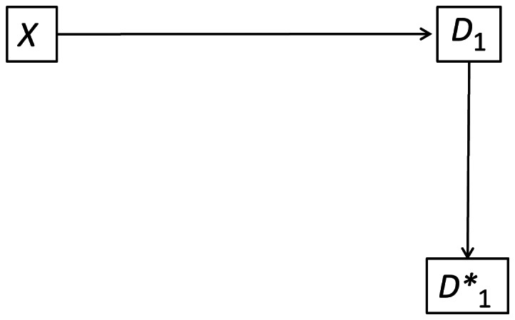
Harvard Study of Moods and Cycles Cohorts 1 (1995­–1997) and 2 (2005–2009), eastern Massachusetts. Directed acyclic graph illustrating potential for exposure misclassification of disease status, D₁, where X represents the geographic location in which the cohort resides, and D*₁ is the observed misclassified version of D₁.

Table 3 shows the risk of screening for MDD or any other SCID-IV condition during 3 years of follow-up. The magnitude of the RDs calculated with this approach is very comparable to the estimated RD, which indicates that differences in the sensitivity of the SCID-IV screening instrument do not seem to contribute to the difference in incident MDD. Women in MC1 were more likely to screen for either MDD or any other SCID-IV condition, which suggests that, independent of imbalance and confounding, women in MC1 still had a greater risk of incident MDD than women in MC2.

Table 3.

Incidence of MDD, SCID Screening for MDD, and Screening for Other SCID Conditions During 3 Years of Follow-up, Harvard Study of Moods and Cycles Cohort 1 (1995–1997) and Cohort 2 (2005–2009), Eastern Massachusetts

Outcome	Risk, %		RD	95% CI	RDAdj.a	95% CI
	MC1 (n = 581)	MC2 (n = 254)
Screening for MDD	13.6	3.8	9.8	5.9, 13.7	7.7	3.1, 12.3
Screening for other SCID condition	12.4	6.5	5.9	1.5, 10.4	4.0	−1.1, 9.1

Abbreviations: CI, confidence interval; MC1, Harvard Study of Moods and Cycles Cohort 1; MC2, Harvard Study of Moods and Cycles Cohort 2; MDD, major depressive order; RD, risk difference; SCID, Structured Clinical Interview for Diagnostic and Statistical Manual of Mental Disorders (Fourth Edition) Axis 1 Diagnoses.

^a Adjusted for propensity score quartiles.

Selection bias: conditioning on participation

Not all women who were invited to enroll in MC1 or MC2 agreed to participate, which raises the potential for selection bias. The proportion of those eligible who actually enrolled differed between MC1 and MC2 (34% vs. 21%). If other covariates affected participation as well as incident depression, selection bias could result. The DAG in Figure 4 illustrates the potential for selection bias due to selective participation in the study. In this figure, the nodes D₀ and D₁ are incident depression at baseline and follow-up, respectively. The node X is, again, the “exposure” of interest—whether a person lives in the geographic region from which the MC1 or MC2 populations were drawn. Unmeasured factors (U) and geographic region (X) affect both incident depression and selection into the study (S). The unmeasured factors giving rise to selection bias could be variables such as genetic predisposition or family history of depression (12). Finally, D₀ influences selection into the study because women with baseline depression were ineligible for the study.

Figure 4.

Harvard Study of Moods and Cycles Cohorts 1 (1995­–1997) and 2 (2005–2009), eastern Massachusetts. Directed acyclic graph illustrating selection bias. Here, D₀ is the baseline depression status, S is selection into the study, D₁ is incident depression during follow-up, U is unmeasured confounding, and X is the geographic location in which the cohort resides. The boxes around S and D₀ indicate that the Harvard Study of Moods and Cycles conditions on these variables.

As explained in Hernan et al. (13), conditioning on a variable that is caused by 2 or more other variables creates a correlation between those upstream variables; even if X and U are independent of each other in the general population, they will be dependent once we have conducted the study and conditioned on the participation node (S). In this example, we speculate that the unmeasured variables decreased the likelihood of women enrolling in the study; furthermore, those in MC1 were more likely to participate than those from the MC2 geographic area. As a result, women who enrolled in the study from MC1 would have a higher prevalence of the unmeasured factor U than women who enrolled in MC2. Given the assumption of no interaction between X and U, a positive correlation would be induced between X and U even if one did not exist in the general population (VanderWeele and Robins (14), theorem 4). Because the factors represented by U were likely to increase the risk of incident depression, our inability to adjust for U would result in a biased estimate of the RD of depression in MC1 versus MC2. Specifically, because of the induced positive correlation between X and U and the positive correlation between U and D₁, we would anticipate the estimated RD to be an overestimate of the true RD (8–10; in particular, see result 1 in VanderWeele et al. (10)). Unlike the results seen in the consideration of unmeasured confounding, this bias is in the direction that could explain the excessively large RD that was observed. Further examination of this type of bias in simulated data is included the Appendix.

Conditioning on baseline depression status

Conditioning on self-selection into the study is a common form of selection bias. However, in the Harvard Study of Moods and Cycles, the design is likely to have created an additional source of selection bias. Like many epidemiologic studies, this study was designed to exclude participants who had experienced the outcome before baseline. As discussed by Hernan et al. (see Figure 6 in Hernan et al.) (13) and Flanders and Klein (15), eliminating those who already have the disease from the study also can induce selection bias. In our study, unmeasured factors (U) are assumed to increase the risk of baseline depression, whereas geographic location (X) is assumed to decrease baseline depression because women in MC1 were anticipated to have lower risk of depression than women in MC2. If we assume that unmeasured causes of depression and geographic location are independent of each other, by eliminating women with depression at baseline, we were enrolling a cohort in MC2 that could have had an induced correlation between those factors. Among women who were free of depression at baseline, those in MC1 could have had a higher prevalence of unmeasured risk factors for depression. Women in MC2 who were prone to depression might have experienced enough stressors in their lives at an early age to trigger depression. As a result, women eligible when the study began were at substantially reduced risk relative to women in MC1. The result of this second, design-induced selection bias is the same as for self-selection bias: The induced positive correlation between X and U combined with the positive association between U and D₁ biased the estimated RD in a positive direction, and the observed association is a likely overestimate of the true RD.

DISCUSSION

In the Harvard Study of Moods and Cycles, a markedly elevated risk of depression was found in a cohort of women from a more affluent area relative to a cohort from a less affluent area. We investigated multiple potential sources of bias as a possible explanation for this finding. Although outcome misclassification cannot be ruled out, examination of a less stringent outcome definition that might not carry stigma did not alter our findings. Our examination of confounding indicated that confounding by measured variables was not responsible for the increased risk in MC1 relative to MC2. We cannot rule out the possibility that part of our observed effect could be due to the greater racial diversity present in the MC2 cohort, given the recent evidence to suggest that African Americans could have a lower prevalence of depression than whites (16); nevertheless, even after adjustment for race in our propensity score models, MC2 still had a decreased risk of depression. Furthermore, by using the theory of signed DAGs developed by VanderWeele et al. (8–10), we argued that unmeasured confounding (due to the unmeasured confounders we specify) was unlikely to have been responsible for our findings.

Two sources of selection bias were possible in our study, and we argued that both of them would bias the effect estimate in the direction we observed. The first source of bias is a common concern in observational epidemiology: Participation in the study is determined by the exposure variable as well as unmeasured covariates that also cause the outcome. The second source of selection bias might be nearly as common but less well recognized. By enrolling only women who had no baseline depression, we created a situation in which women who participated in MC2 could have been healthier than women who participated in MC1, and furthermore, in which the unmeasured healthiness reduced the risk of depression during follow-up in MC2 relative to MC1.

Previous research has suggested that some people might have a predisposition toward depression and that environmental stressors lead to increased risk (17–19). Women living in lower socioeconomic conditions could be more likely to have experienced more significant stressors at earlier ages than women who live in higher socioeconomic conditions. In a lower socioeconomic status environment, enough significant stressors could occur to trigger depression at an earlier age. By limiting enrollment in our studies to women 36 years of age or older with no lifetime history of depression, we inadvertently might have selected a healthier group of women in MC2 because women with a predisposition toward depression in that cohort would have been more likely to have already experienced depression.

We emphasize that the sources of biases that we discuss do not act in isolation. Rather, the total bias is a combination of the individual sources. Of particular importance in this regard are the 2 sources of selection bias. Although each of them could produce a modest amount of bias individually, their joint effect might be substantially larger (as we illustrate in the Appendix). We note, as well, that the conclusions reached depend on the assumptions made in our DAG (such as Figure 4), as well as the direction of the associations, which are unobserved, and assumptions of statistical independence. Different assumptions about the sign of the associations or different DAGs could result in different inferences. In the analysis of unmeasured confounding, for instance, some unmeasured confounders could conceivably be positively associated with X in Figure 1. This would induce a bias that could help explain our observed result. Furthermore, not all analyses involving the Harvard Study of Moods and Cycles will be susceptible to each of the biases outlined above. A substantial rationale for this cohort study was to examine the impact of various factors on the menopausal transition. Because women were enrolled largely before onset of menopause, limiting the study to women without depression at baseline might produce little bias in these analytical assessments.

Despite nearly identical enrollment procedures in MC1 and MC2, we were surprised to find far lower rates of depression in MC2, the cohort with greater racial diversity and lower socioeconomic status. Our surprise was not diminished by our inability to explain this discrepancy by observed demographic differences between the 2 cohorts. Furthermore, little evidence was found to suggest that women in MC2 were simply less likely to report depressive symptoms; examining less stringent criteria did not decrease the observed difference in risk of depression between MC1 and MC2. Thus, we propose that the differences found were the consequence of selection bias. Investigators exploring associations that involve disparate racial and economic populations, despite identical recruitment methods, should be aware of this potential bias.

APPENDIX

In this appendix, we illustrate the impact of selection bias in simulated data. We simulate data consistent with the DAG in Figure 4. In the simulated data, we assume that the main exposure, X, has no effect on depression at follow-up, D₁. This allows us to quickly assess the impact of selection bias on the effect of X on D₁, under the null hypothesis. The code below is annotated R (R Foundation for Statistical Computing, Vienna, Austria) code, with the symbol “#” preceding comments.

# First, we simulate data for the unmeasured confounder, u, and the exposure, x. The prevalence of the confounder is 0.5, and the 10^5 samples are generated to reduce random noise.

u<-rbinom(10^5,1,.5)

x<-rbinom(10^5,1,.5)

# Next, we simulate baseline disease status with the log(OR) for U = −2 and log(OR) for X = 2.

lp.d = 2*u-2*x

d0=rbinom(10^5,1,exp(lp.d)/(1+exp(lp.d)))

# Next, we simulate data for the study selection indicator, S.

lp.s=-2*u+2*x

s=rbinom(10^5,1,exp(lp.s)/(1+exp(lp.s)))

# Because individuals with baseline disease were not eligible for the study, we set S equal to zero if the individual has baseline disease.

s[d0==1]<-0

# Finally, we simulate outcome data. The true log(OR) is 1.0 for U and 0.0 for X.

d1=rbinom(10^5,1,exp(u)/(1+exp(u)))

# We can double-check that U and X are marginally independent. In the example we ran, cor = −0.004, approximately zero.

cor(u,x)

# We can see that among the people in the study (s = 1), a correlation exists between U and X. In the example we ran, cor = 0.1957.

cor(u[s==1],x[s==1])

# We can see that among the people without disease at baseline (D₀ = 0), a correlation exists between U and X. In this example, cor = 0.1674.

cor(u[d0==0],x[d0==0])

# We can compare the log(OR) for the effect of X on D₁ among the whole sample (log(OR)=0.011, in this example). Note that there is no confounding of this effect, given the DAG in Figure 4, so there is no need to include U in the regression.

glm(d1∼x,family=binomial)$coef

# Last, we can examine the effect of X on D₁ among those who are selected into the study (S = 1). In this example, the log(OR) = 0.20.

glm(d1[s==1]∼x[s==1],family=binomial)$coef

This example illustrates the general principle that selection bias resulting from the DAG we specify can result in substantial bias in the effect of X on D₁. We have taken care in this example to specify effects that are consistent with the sign of the bias we specified in the paper. Different assumptions about the prevalences and true effects will result in differing extent of bias. Extensive simulations (as well as theory) indicate that the direction of the bias is consistent, regardless of prevalences, as long as the sign of the log(OR) remains as specified.

REFERENCES

- 1.Harlow BL, Wise LA, Otto MW, et al. Depression and its influence on reproductive endocrine and menstrual cycle markers associated with perimenopause: the Harvard Study of Moods and Cycles. Arch Gen Psychiatry. 2003;60(1):29–36. doi: 10.1001/archpsyc.60.1.29. [DOI] [PubMed] [Google Scholar]
- 2.Cohen LS, Soares CN, Vitonis AF, et al. Risk for new onset of depression during the menopausal transition. The Harvard Study of Moods and Cycles. Arch Gen Psychiatry. 2006;63(4):385–390. doi: 10.1001/archpsyc.63.4.385. [DOI] [PubMed] [Google Scholar]
- 3.Bromberger JT, Harlow S, Avis N, et al. Racial/ethnic differences in the prevalence of depressive symptoms among middle-aged women: the Study of Women's Health Across the Nation (SWAN) Am J Public Health. 2004;94(8):1378–1385. doi: 10.2105/ajph.94.8.1378. [DOI] [PMC free article] [PubMed] [Google Scholar]
- 4.First MB, Spitzer RL, Gibbon M, et al. New York, NY: Biometrics Research Department, New York State Psychiatric Institute; 1996. Williams Structured Clinical Interview for DSM-IV Axis I Disorders—Non-patient Edition (SCID-I/NP, Version 2.0) [Google Scholar]
- 5.Rosenbaum PR, Rubin DB. The central role of the propensity score in observational studies for causal effects. Biometrika. 1983;70(1):41–55. [Google Scholar]
- 6.Belle D, Doucet J. Poverty, inequality, and discrimination as sources of depression among U.S. women. Psychol Women Q. 2003;27(2):101–113. [Google Scholar]
- 7.Arah OA, Chiba Y, Greenland S. Bias formulas for external adjustment and sensitivity analysis of unmeasured confounders. Ann Epidemiol. 2008;18(8):637–646. doi: 10.1016/j.annepidem.2008.04.003. [DOI] [PubMed] [Google Scholar]
- 8.VanderWeele TJ. The sign of the bias of unmeasured confounding. Biometrics. 2008;64(3):702–706. doi: 10.1111/j.1541-0420.2007.00957.x. [DOI] [PubMed] [Google Scholar]
- 9.VanderWeele TJ, Robins JM. Signed directed acyclic graphs for causal inference. J R Stat Soc Series B Stat Methodol. 2010;72(1):111–127. doi: 10.1111/j.1467-9868.2009.00728.x. [DOI] [PMC free article] [PubMed] [Google Scholar]
- 10.VanderWeele TJ, Hernán M, Robins JM. Causal directed acyclic graphs and the direction of unmeasured confounding. Epidemiology. 2008;19(5):720–728. doi: 10.1097/EDE.0b013e3181810e29. [DOI] [PMC free article] [PubMed] [Google Scholar]
- 11.Dowd JB, Todd M. Does self-reported health bias the measurement of health inequalities in U.S. adults? Evidence using anchoring vignettes from the Health and Retirement Study. J Gerontol B Psychol Sci Soc Sci. 2011;66(4):478–489. doi: 10.1093/geronb/gbr050. [DOI] [PubMed] [Google Scholar]
- 12.Kendler KS, Gatz M, Gardner CO, et al. A Swedish national twin study of lifetime major depression. Am J Psychiatry. 2006;163(1):109–114. doi: 10.1176/appi.ajp.163.1.109. [DOI] [PubMed] [Google Scholar]
- 13.Hernan MA, Hernandez Diaz S, Robins JM. A structural approach to selection bias. Epidemiology. 2004;15(5):615–625. doi: 10.1097/01.ede.0000135174.63482.43. [DOI] [PubMed] [Google Scholar]
- 14.VanderWeele TJ, Robins JM. Minimal sufficient causation and directed acyclic graphs. Ann Stat. 2009;37(3):1437–1465. [Google Scholar]
- 15.Flanders WD, Klein M. Properties of 2 counterfactual effect definitions of a point exposure. Epidemiology. 2007;18(4):453–460. doi: 10.1097/01.ede.0000261472.07150.4f. [DOI] [PubMed] [Google Scholar]
- 16.Riolo SA, Nguyen TA, Greden JF, et al. Prevalence of depression by race/ethnicity: findings from the National Health and Nutrition Examination Survey III. Am J Public Health. 2005;95(6):998–1000. doi: 10.2105/AJPH.2004.047225. [DOI] [PMC free article] [PubMed] [Google Scholar]
- 17.McLaughlin KA, Kubzansky LD, Dunn EC, et al. Childhood social environment, emotional reactivity to stress, and mood and anxiety disorders across the life course. Depress Anxiety. 2010;27(12):1087–1094. doi: 10.1002/da.20762. [DOI] [PMC free article] [PubMed] [Google Scholar]
- 18.Wichers M, Geschwind N, Jacobs N, et al. Transition from stress sensitivity to a depressive state: longitudinal twin study. Br J Psychiatry. 2009;195(6):498–503. doi: 10.1192/bjp.bp.108.056853. [DOI] [PubMed] [Google Scholar]
- 19.Belsky J, Pluess M. Beyond diathesis stress: differential susceptibility to environmental influences. Psychol Bull. 2009;135(6):885–908. doi: 10.1037/a0017376. [DOI] [PubMed] [Google Scholar]