Origin of seasonal predictability for summer climate over the Northwestern Pacific

Abstract

Summer climate in the Northwestern Pacific (NWP) displays large year-to-year variability, affecting densely populated Southeast and East Asia by impacting precipitation, temperature, and tropical cyclones. The Pacific–Japan (PJ) teleconnection pattern provides a crucial link of high predictability from the tropics to East Asia. Using coupled climate model experiments, we show that the PJ pattern is the atmospheric manifestation of an air–sea coupled mode spanning the Indo-NWP warm pool. The PJ pattern forces the Indian Ocean (IO) via a westward propagating atmospheric Rossby wave. In response, IO sea surface temperature feeds back and reinforces the PJ pattern via a tropospheric Kelvin wave. Ocean coupling increases both the amplitude and temporal persistence of the PJ pattern. Cross-correlation of ocean–atmospheric anomalies confirms the coupled nature of this PJIO mode. The ocean–atmosphere feedback explains why the last echoes of El Niño–Southern Oscillation are found in the IO-NWP in the form of the PJIO mode. We demonstrate that the PJIO mode is indeed highly predictable; a characteristic that can enable benefits to society.

Summer is the rainy season for East Asia, and the precipitation supports the livelihood of over 1 billion people. The East Asian summer monsoon displays large interannual variability, and the prediction of summer climate anomalies is an urgent societal need. The prolonged rainy season in 1993 caused a nation-wide harvest failure in Japan, instrumental in opening the domestic rice market by forcing large-scale imports (1). The great Yangtze River flood in the summer of 1998 left 15 million people homeless and triggered a national effort to restore wetlands (2). Dry summer, in contrast, is often accompanied by heat waves as in 2004, causing a large number of victims of heat stroke and a risk of electric power shortage. El Niño–Southern Oscillation (ENSO) is the leading predictor for East Asian summer climate (3). Indeed, summer atmospheric circulation and surface temperature over Japan and Yangtze River discharge are significantly correlated with ENSO at a two-season lag (Fig. 1A).

Fig. 1.

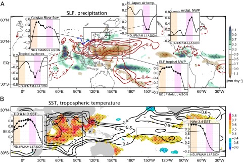
Observed correlations and regressed anomalies with respect to NDJ Niño 3.4 SST. (A and B) Precipitation regressions (shading) and SLP correlations (contours) (A) and correlations of SST (shading) and tropospheric temperature (contours) (B) in subsequent JJA. Stippling indicates 95% confidence of shaded fields. Contours are drawn for ±0.4, ±0.5, ±0.6, …. Insets show 3-mo running correlations for ENSO-peak to -decay seasons. (A, anticlockwise from top left) Yangtze River flow, TC genesis, SLP over [10°–25°N, 110°–160°E], 1,000-hPa vorticity over [32.5°–42.5°N, 115°–145°E], and land-surface air temperature over [38°–46°N, 138°–148°E]. (B) (Left to Right) Tropical (20°S–20°N, 40°–100°E; solid lines) and northern (5°–25°N, 40°–100°E; dashed lines) IO and Niño 3.4 SST. Open (solid) circles indicate 90% (95%) confidence.

ENSO is the dominant mode of interannual variability with global influences. ENSO is strongly tied to the annual cycle, growing during boreal summer, peaking in winter, and decaying in the following spring (Fig. 1B) (4). By the subsequent summer, ENSO itself has dissipated in the equatorial Pacific, but its climatic influence lingers (Fig. 1) (5, 6). A global survey reveals that in the El Niño-decay summer, surface climate anomalies are most robust over the Indo-Northwestern Pacific (NWP) region (Fig. 1). In such a summer, Indian Ocean (IO) sea surface temperature (SST) is anomalously high (Fig. 1B) (5, 7), with suppressed convection and an anomalous anticyclonic circulation over the tropical NWP (8) extending to the northern Bay of Bengal (Fig. 1A) (9). The tropical NWP anomalies further affect East Asia through an atmospheric meridional teleconnection called the Pacific–Japan (PJ) pattern (10, 11). A question arises, which is addressed here: Why are these last echoes of ENSO confined to the Indo-NWP warm pool? It may be tempting to invoke ocean thermal inertia as the cause of the long persistence of IO SST, but this simple explanation is challenged by the facts that the rate of El Niño-induced SST warming over the northern IO peaks after ENSO has dissipated and that the persistence is sustained by reduced turbulent heat flux due to the relaxed southwesterly monsoon (12). We show here with coupled general circulation model (GCM) experiments that the aforementioned ocean–atmospheric anomalies are intrinsically coupled. We demonstrate that this unique coupled mode over the Indo-NWP region is distinct from and can exist without ENSO. In nature, however, ENSO excites this coupled mode, giving rise to the temporal persistence and spatial coherence of Indo-NWP climate anomalies. We show that the coupled mode is predictable, giving us hopes for skillful seasonal forecast over the densely populated region.

This study uses the Geophysical Fluid Dynamics Laboratory (GFDL) Coupled Model version 2.1 (CM2.1) (13) and its atmospheric component, the Atmospheric Model version 2.1 (AM2.1) (14). CM2.1 is among the best models in simulating atmospheric variability over the summer NWP (15). Two sets of “partial coupling” experiments are performed with CM2.1, in which the SST evolution in the equatorial eastern Pacific is specified, but the atmosphere and ocean are fully coupled outside. In the Pacific Ocean–Global Atmosphere (POGA) experiment, SST anomalies follow observed historical values over the equatorial eastern Pacific in all nine member runs, whereas in the other experiment named NoENSO, interannual variability of SST is suppressed over the same region (Materials and Methods). By suppressing internal variability, the POGA ensemble mean isolates ENSO-induced variability. NoENSO represents variability independent of ENSO, which is equivalent to intermember variability in POGA. To isolate atmospheric internal variability, we conduct an AM2.1 experiment named aCLIM, where the CM2.1 climatological SST is prescribed globally.

Atmospheric Mode

We perform an empirical orthogonal function (EOF) analysis of 850 hPa vorticity to extract the dominant mode of variability over the summer NWP [June–July–August (JJA)] (Materials and Methods). In observations, the leading mode (EOF1) features meridional dipoles in lower tropospheric circulation and precipitation between the tropics (10°–25°N) and midlatitudes (25°–40°N) (Fig. 2 A and B) (10, 11). These features characterize the PJ pattern, which provides a crucial connection between the tropics and midlatitudes. In its positive phase (Fig. 2), the PJ pattern brings a wetter and cooler summer to central China, Korea, and Japan (SI Text and Fig. S1) (16, 17). Tropical cyclone (TC) activity significantly decreases over the NWP (Fig. S1) (18). Conversely, the pattern in its negative phase causes droughts and heat waves in the midlatitudes with enhanced TC activity. The corresponding principal component (PC1) is strongly positive (negative) in both 1993 and 1998 (in 2004) (Fig. 2I). The PJ pattern is correlated with ENSO (e.g., 1998) but can develop without it (e.g., 1993 and 2004). The rainfall distribution of the vorticity-based EOF1 is slightly different from the ENSO pattern over the tropical IO and Maritime Continent (Fig. 2B vs. Fig. 1A).

Fig. 2.

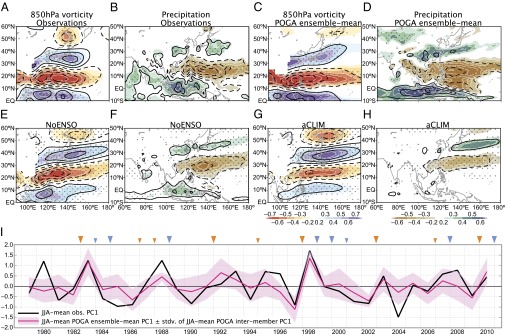
(A–H) Anomalies of (A, C, E, and G) 850-hPa vorticity and (B, D, F, and H) precipitation associated with EOF1s of NWP 850-hPa vorticity. Shown are (A and B) observations, (C and D) POGA ensemble mean, (E and F) NoENSO, and (G and H) aCLIM. Shading indicates correlations, with stippling representing 95% statistical confidence, whereas contours show regressed anomalies, all with respect to PC1s. Contours are plotted for (A, C, E, and G) ±0.5, ±1.5, ±2.5, … ×10⁻⁶ s^–1 and (B, D, F, and H) ±0.5, ±1.5, ±2.5, … mm⋅d^–1. (I) The corresponding PC1 time series in observations (black) and POGA (red), averaged for JJA. Shading represents ±1 SD of intermember PC1 in POGA. Orange and blue triangles at the top indicate El Niño and La Niña events (large triangles, strong to moderate; small triangles, weak), respectively, based on NDJ Niño 3.4 SST.

The PJ pattern appears as EOF1 of each experiment (Fig. 2 C–H), well separated from higher modes. The model and observational EOF1 patterns are highly alike (Table S1). This pattern similarity is particularly striking in the mid- to high latitudes whereas the tropical amplitude and spatial pattern vary somewhat in accordance with the degree of SST influence. The dominance of the PJ pattern in aCLIM indicates that it can arise as an atmospheric internal mode in the absence of SST variability (11).

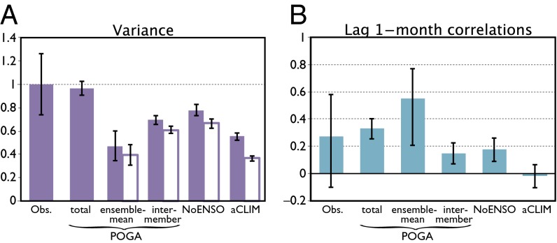
The total PJ variance in POGA agrees with observations remarkably well (Fig. 3A). The POGA ensemble mean accounts for ∼40% of the monthly PJ variance (Fig. 3A and Table 1). It is correlated with the ENSO index [Niño 3.4 (5°S–5°N, 150°–90°W) SST] in the preceding boreal winter [November–December–January (NDJ)] at 0.66 (P < 0.01) when averaged for the summer season (Fig. S2), consistent with observational (19) and prediction (3, 20) studies. The POGA ensemble-mean PC1 is also significantly correlated with observations at 0.71 (P < 0.01) for seasonal mean (Fig. 2I).

Fig. 3.

(A) Variance explained by (solid bars) EOF1 of individual variability and (open bars) projections onto the EOF1 pattern of POGA total variability, both scaled with variance of observational EOF1 (Materials and Methods). (B) One-month–lagged autocorrelations of PC1s. Error bars (A) are derived from North’s rule and (B) represent 95% intervals.

Table 1.

Variance fractions of the PJ pattern explained by variability components

Variability component	Percent
ENSO-forced, air–sea coupled	39.2
Non-ENSO forced
Air–sea coupled	24.5
Atmospheric internal	36.3

See Materials and Methods for details.

Coupled Mode

PJ variability in aCLIM is only ∼36% of the total variance in POGA (Fig. 3A and Table 1). Without SST forcing, this purely atmospheric internal mode shows vanishing month-to-month persistence, in sharp contrast with significant persistence in either POGA ensemble mean or total variability (Fig. 3B). Allowed to interact with the ocean, PJ variability in NoENSO is significantly stronger than in aCLIM by a factor of 1.4∼1.8 (Fig. 3A) and, in addition, bears considerable month-to-month persistence (Fig. 3B). These changes in amplitude and temporal persistence are suggestive of coupled interaction between the PJ pattern and the ocean.

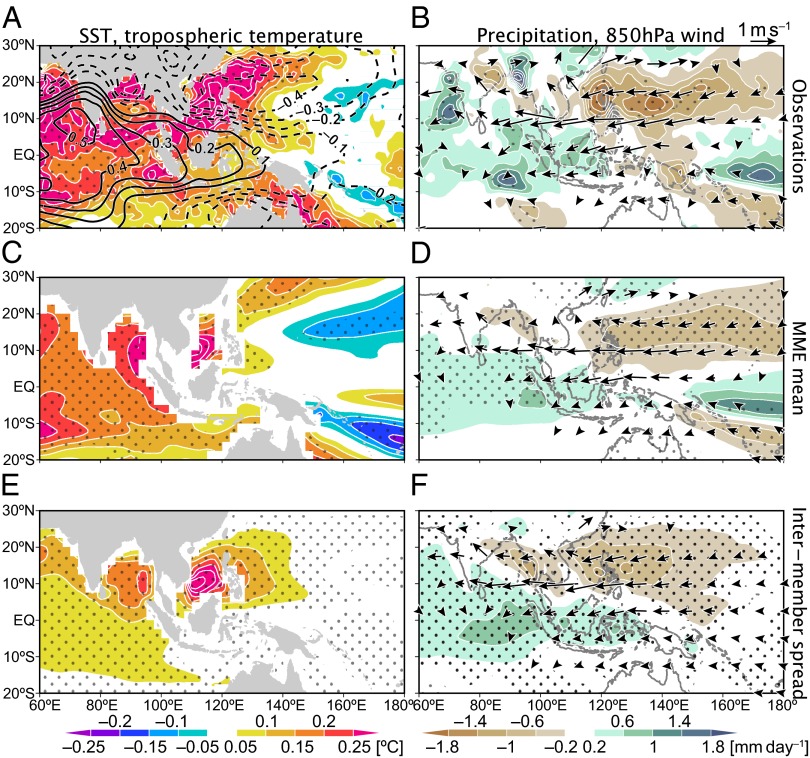
The spatial structures of ocean–atmospheric anomalies suggest a positive feedback. Anomalous anticyclonic circulation of the PJ’s tropical (10°–25°N) lobe extends westward to the northern IO, as a cold Rossby wave response to precipitation decrease over the NWP (Fig. 4B, SI Text, and Fig. S3A) (21). The associated easterly anomalies on the southern flank weaken the climatological monsoon westerlies, reducing surface evaporation and increasing SST over the northern IO and the South China Sea (SCS) (Fig. 4A). The northeasterly anomalies reach the equator, helping suppress evaporation, and increase SST around the Maritime Continent. Reduction of cloud amount contributes to the warming of the northern SCS and Bay of Bengal through insolation (Fig. S4). Positive SST anomalies thus induced heat the troposphere via moist adiabatic adjustment (22) and excite an atmospheric warm Kelvin wave extending eastward along the equator (Fig. 4B, SI Text, and Fig. S3B). Over the off-equatorial NWP, the Kelvin wave suppresses precipitation by inducing surface Ekman divergence (19). Weak negative SST anomalies in the NWP east of 140°E may also contribute to this convective suppression (23). The resultant change in latent heat release in the troposphere is the primary energy source for the PJ pattern (11). This ocean–atmosphere feedback amplifies the initial PJ pattern. We have confirmed that observed PJ events in non-ENSO years feature a similar structure (SI Text and Figs. S5 and S6).

Fig. 4.

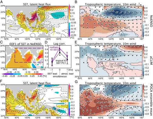
(A, B, and E–G) Regressed anomalies of (A and F) SST (shading) and latent head flux (contours; positive downward), and (B, E, and G) correlations of tropospheric temperature (shading) and 10-m wind velocity (arrows) in JJA, against (A and B) NoENSO PC1, (E) aCLIM PC1, and (F and G) Niño 3.4 SST in preceding NDJ in ensemble-mean POGA. Contours in A and F are drawn for ±1, ±3, ±5, … W⋅m^–2. Stippling indicates 95% confidence of (A and F) latent heat flux and (B, E, and G) tropospheric temperature. In G, the tropical (30°S–30°N) average has been removed from tropospheric temperature. (C and D) SST EOF1 in the tropical IO (C) and lead–lag correlations of the corresponding PC and SST in [0°–25°N, 60°–120°E] (D) with PC1 of NWP 850-hPa vorticity in NoENSO. Error bars represent 95% intervals.

The remote effect of the northern IO SST on convection over the NWP has been confirmed with atmospheric GCMs (19, 24). In the absence of SST forcing in aCLIM, the Kelvin wave and precipitation anomalies are missing along the equator (Figs. 2H and 4E). Interestingly, the ocean–atmosphere coupling extends the PJ tropical lobe farther westward (Fig. 4 B and E), consistent with our linear model experiment (SI Text and Fig. S3B).

We test the hypothesis of ocean–atmosphere coupling by calculating lead–lag correlation in NoENSO between the PJ pattern and SST averaged in the northern IO and the SCS. If positive feedbacks dominate, this correlation would peak at zero lag, whereas negative feedbacks would cause the correlation to change sign near zero lag (25). In NoENSO, the correlation maximizes at zero lag (Fig. 4D), indicating the coupling between the PJ pattern and IO SST (hereafter the PJIO mode). Correlation also peaks at zero lag if the ocean index is extracted with an EOF analysis of SST variability over the IO and SCS (Fig. 4C). The correlations are positive when the atmosphere leads ocean by 1 mo (Fig. 4D), suggesting that chaotic variability of the atmosphere triggers the PJIO mode in NoENSO. The interaction with ocean increases the amplitude and temporal persistence of PJ variability (Fig. 3).

Whereas the PJIO mode can exist without external forcing, ENSO efficiently excites this mode by inducing IO SST anomalies (5, 6, 19) as an initial perturbation (Fig. 1). Indeed, the spatial pattern of POGA ensemble-mean anomalies in ENSO-decay summer (Fig. 4 F and G) resembles the PJIO mode in NoENSO (Fig. 4 A and B), especially north of the equator. The total PJ variance in POGA can be decomposed into ENSO-forced, non-ENSO but ocean–atmosphere coupled, and atmospheric internal components. The non-ENSO coupled component contributes one-quarter of the total PJ variance in POGA, comparable to the other two components (Table 1).

Origin of Seasonal Predictability

The coupled PJIO mode brings predictability to summer climate over the NWP. We evaluate this hypothesis in predictions by 14 coupled GCMs that are initialized on May 1 each year from around 1980 to the 2000s. A singular value decomposition (SVD) analysis extracts the leading covariability mode of 850 hPa vorticity over the NWP and SST in the northern IO in JJA (Materials and Methods). The PJIO mode emerges both in multimodel ensemble (MME)-mean (i.e., predicted signal) (Fig. 5 C and D) and intermember variability (uncertainty of the prediction) in each model (Figs. S7 and S8) and in the multimodel grand ensemble (Fig. 5 E and F) (26). (As in POGA intermember variability, the leading mode of intermember variability in prediction models strongly resembles the PJIO mode in the NoENSO experiment.) At first it may appear peculiar that both the prediction and its uncertainty project onto the same mode, but this similarity arises from the dominance of the PJIO mode in the summer Indo-NWP region and its coupled nature. Initial anomalies, especially those of IO SST, set the PJIO mode in motion, although its precise evolution is chaotic and sensitive to initial atmospheric perturbations.

Fig. 5.

(A–F) Anomalies of (A, C, and E) SST (shading), (B, D, and F) precipitation (shading), and 850-hPa wind velocity (arrows) regressed onto SVD1s of IO SST and NWP 850-hPa vorticity in JJA, based on (A and B) observations and (C and D) MME mean and (E and F) grand ensemble of intermember variance of seasonal predictions. Contours in A indicate tropospheric temperature correlation with its tropical (30°S–30°N) average subtracted and are drawn for ±0.1, ±0.2, ±0.3, …. Stippling indicates 95% statistical confidence of shaded fields.

The PJIO mode in the MME-mean prediction (Fig. 5 C and D) is temporally correlated with observations (Fig. 5 A and B) at 0.72 for vorticity and 0.90 for SST in seasonal mean. It is also correlated with the ENSO index in the preceding boreal winter at 0.72 (0.88) for vorticity (SST). These correlations are all significant at P < 0.01, indicating a high predictability of the PJIO mode in ENSO-decay summer. The PJIO mode enables ENSO to induce its last echo over the Indo-NWP in boreal summer (Fig. 1), bringing seasonal predictability to the region.

Summary and Discussion

Our analyses reveal a unique coupled mode over the Indo-NWP warm pool during boreal summer that arises from interaction between IO SST and the PJ pattern. This PJIO coupled mode can exist without but is efficiently excited by ENSO. In total, the PJIO coupled mode, forced plus unforced, amounts to two-thirds of the PJ variability in POGA (Fig. 3A and Table 1). The positive ocean–atmosphere feedback reduces the damping on the mode, making it the last echo of ENSO (Fig. 1). The coupled mode brings seasonal predictability to summer NWP climate. Suppressing this mode lowers the predictability substantially as shown by an IO-decoupled seasonal hindcast (3). The coupling also enhances the westward expansion of the PJ tropical lobe, thereby contributing to predictability over the Indochina Peninsula and the Gangetic Plain (9).

Local correlation between precipitation and SST is often used as a test for ocean–atmosphere coupling (27). The PJIO mode is an exception to this rule, because the nonlocal nature of the interaction does not require local positive precipitation–SST correlations. The spatial structure of the PJIO mode explains the observed negative local correlation over the tropical NWP in ENSO-decay summers (28, 29). In ENSO-developing summers the local correlation is positive (29), resulting in an insignificant local correlation for all years.

Summer climate prediction remains a grand challenge for Southeast and East Asia, regions that more than 1 billion people call home. The coupled nature of the PJIO mode, with an atmospheric center of action over East Asia, offers hope and points to ways forward in meeting the prediction challenge. Although ENSO is a major driver for East/Southeast Asian climate predictability, our study suggests that properly initializing the PJIO mode can improve seasonal prediction considerably: whereas 39% of the PJ variance is explained by ENSO, the non-ENSO coupled mode contributes an additional 25% (Table 1). In fact, in five weak ENSO summers (1986, 1990, 1993, 1994, and 1996, for which Niño 3.4 SSTs in the preceding NDJ and simultaneous JJA are both within ±0.7 times the SD, of 20 hindcasted years), correlation between seasonal-mean PC1s for observations and the MME is 0.85. We note that a useful prediction needs to be accompanied by a good estimate of uncertainty. A nine-member atmospheric experiment, where POGA ensemble-mean SST is prescribed globally, underestimates the uncertainty of the PJ prediction because the ocean and atmosphere are decoupled (SI Text). Over the summer NWP, prediction uncertainty is organized into and determined by the PJIO mode. The recognition of the coupled nature of the PJIO mode will enable the identification of optimal perturbations, a method that proves useful in estimating error growth and uncertainty of seasonal predictions (30, 31).

Materials and Methods

Observational Datasets.

We use monthly sea-level pressure (SLP), tropospheric temperature, vorticity and wind velocity of 25-y Japanese Reanalysis (JRA-25) (http://jra.kishou.go.jp) (32), Climate Prediction Center Merged Analysis of Precipitation (CMAP) (www.cpc.ncep.noaa.gov/products/global_precip/html/wpage.cmap.html) (33), and Hadley Centre Sea Ice and SST (HadISST1) (www.metoffice.gov.uk/hadobs/hadisst/) (34) datasets. JRA-25 and CMAP (HadISST1) are provided with 2.5° × 2.5° (1° × 1°) resolution. Our analysis covers a 32-y period of 1979–2010. Other data used include Yangtze River flow at Datong station (∼500 km inland from the estuary) from 1980 to 2009, University of Delaware surface air temperature for 1978–2008 on a 0.5° × 0.5° grid (http://climate.geog.udel.edu/~climate/) (35), and NWP TC track records for 1978–2010 from the Regional Specialized Meteorological Center Tokyo Typhoon Center (www.jma.go.jp/jma/jma-eng/jma-center/rsmc-hp-pub-eg/RSMC_HP.htm). We examine TCs with wind speed exceeding 17.2 m⋅s^–1.

Model Experiments.

The atmospheric resolution in GFDL CM2.1 (13) and AM2.1 (14) is 2.5° × 2° in longitude–latitude with 24 vertical levels. The oceanic resolution in CM2.1 is 1° in longitude and latitude, with meridional resolution equatorward of 30° becoming progressively finer to 1/3° at the equator, and there are 50 oceanic levels vertically.

Using CM2.1, we conduct the POGA (NoENSO) experiment, where SST over the deep tropical eastern Pacific is restored to the model climatology plus (without) historical anomaly, by overriding surface sensible heat flux to ocean () with

Here the prime indicates the anomaly and asterisks represent model-diagnosed values; T denotes SST, and the reference temperature anomaly T′ is obtained from observations in POGA whereas T′ = 0 in NoENSO. The model anomaly is the deviation from a 200-y monthly model climatology. c is specific heat, D = 50 m represents the typical depth of the ocean-mixed layer, and τ = 10 d represents the restoring timescale. Fig. S2 shows the region where SST is restored; within the inner box α = 1, and α linearly reduces to zero in the buffer zone (five and six grid points in zonal and meridional directions, respectively) from the inner to the outer boxes. This restoring reduces interannual SD of NDJ Niño 3.4 SST in NoENSO to 4.2% of the observed value. We perform an additional atmospheric experiment (aCLIM) by prescribing the CM2.1 SST climatology globally to AM2.1.

The POGA experiment is made of nine member runs for 1979–2010, whereas NoENSO and aCLIM are each a single-member integration of 194 y long. CM2.1 has been appropriately spun up before the POGA and NoENSO experiments.

Seasonal Predictions.

The prediction models are those that were used in the Climate Prediction and its Application to Society (CliPAS) project (36) and in the Development of a European Multimodel Ensemble System for Seasonal to Interannual Prediction (DEMETER) project (37). See SI Text for individual models analyzed.

Leading Mode of Variability over the Summer Indo-NWP.

An EOF analysis of monthly 850-hPa vorticity over the NWP (0°–60°N, 100°–160°E) for JJA extracts the PJ pattern as EOF1 (11). We apply this EOF analysis to JRA-25, POGA ensemble-mean, intermember and total (ensemble-mean plus intermember), NoENSO, and aCLIM variability. Fig. 3A shows the corresponding eigenvalues scaled with that of observational EOF1. The EOF1 pattern differs slightly among experiments and from observations (Table S1). For a fair comparison, we project POGA ensemble-mean, NoENSO, and aCLIM variability onto the common pattern of POGA total variance EOF1 (Fig. 3A) and evaluate the relative contributions of ENSO-forced, non-ENSO forced but air–sea coupled, and atmospheric internal components as POGA ensemble-mean, NoENSO minus aCLIM, and aCLIM, respectively (Table 1).

We also apply an EOF analysis to monthly SST over the tropical IO (10°S–30°N, 40°–120°E) in NoENSO (Fig. 4 C and D).

We perform SVD analyses between monthly SST over the tropical IO-SCS (10°S–30°N, 40°–120°E) and 850-hPa vorticity over the NWP (0°–60°N, 100°–160°E) for JJA to extract the coupled mode from observations, POGA ensemble mean, and MME mean and grand ensemble of intermember variance of seasonal predictions. For the grand ensemble of intermember predictions, we have removed the ensemble mean for each model and then accumulated the covariance of all of the models. Regression and correlation maps are plotted against the SST time series.

References

- 1.Hosoe N. Crop failure, price regulation, and emergency imports of Japan’s rice sector in 1993. Appl Econ. 2004;36(10):1051–1056. [Google Scholar]
- 2.Zong Y, Chen X. The 1998 flood on Yangtze, China. Nat Hazards. 2000;22(2):165–184. [Google Scholar]
- 3.Chowdary JS, et al. Predictability of Northwest Pacific climate during summer and the role of the tropical Indian Ocean. Clim Dyn. 2011;36(3-4):607–621. [Google Scholar]
- 4.Larkin NK, Harrison DE. ENSO warm (El Niño) and cold (La Niña) event life cycles: Ocean surface anomaly patterns, their symmetries, asymmetries, and implications. J Clim. 2002;15(10):1118–1140. [Google Scholar]
- 5.Klein SA, Soden BJ, Lau N-C. Remote sea surface temperature variations during ENSO: Evidence for a tropical atmospheric bridge. J Clim. 1999;12(4):917–932. [Google Scholar]
- 6.Lau N-C, Nath MJ. Atmosphere-ocean variations in the Indo-Pacific sector during ENSO episodes. J Clim. 2003;16(1):3–20. [Google Scholar]
- 7.Yang J, Liu Q, Xie S-P, Liu Z, Wu L. Impact of the Indian Ocean SST basin mode on the Asian summer monsoon. Geophys Res Lett. 2007;34(2):L02708. [Google Scholar]
- 8.Wang B, Wu R, Li T. Atmosphere–warm ocean interaction and its impact on Asian–Australian monsoon variation. J Clim. 2003;16(8):1195–1211. [Google Scholar]
- 9.Mishra V, Smoliak BV, Lettenmaier DP, Wallace JM. A prominent pattern of year-to-year variability in Indian Summer Monsoon Rainfall. Proc Natl Acad Sci USA. 2012;109(19):7213–7217. doi: 10.1073/pnas.1119150109. [DOI] [PMC free article] [PubMed] [Google Scholar]
- 10.Nitta T. Convective activities in the tropical western Pacific and their impact on the Northern Hemisphere summer circulation. J Meteorol Soc Jpn. 1987;65(3):373–390. [Google Scholar]
- 11.Kosaka Y, Nakamura H. Mechanisms of meridional teleconnection observed between a summer monsoon system and a subtropical anticyclone. Part I: The Pacific-Japan pattern. J Clim. 2010;23(19):5085–5108. [Google Scholar]
- 12.Du Y, Xie S-P, Huang G, Hu K. Role of air–sea interaction in the long persistence of El Niño-induced north Indian Ocean warming. J Clim. 2009;22(8):2023–2038. [Google Scholar]
- 13.Delworth TL, et al. GFDL’s CM2 global coupled climate models. Part I: Formulation and simulation characteristics. J Clim. 2006;19(5):643–674. [Google Scholar]
- 14.Anderson JL, et al. The new GFDL global atmosphere and land model AM2/LM2: Evaluation with prescribed SST simulations. J Clim. 2004;17(24):4641–4673. [Google Scholar]
- 15.Kosaka Y, Nakamura H. Dominant mode of climate variability, intermodel diversity, and projected future changes over the summertime western North Pacific simulated in the CMIP3 models. J Clim. 2011;24(15):3935–3955. [Google Scholar]
- 16.Huang R, Sun F. Impacts of the tropical western Pacific on the East Asian summer monsoon. J Meteorol Soc Jpn. 1992;70(1):243–256. [Google Scholar]
- 17.Wakabayashi S, Kawammura R. Extraction of major teleconnection patterns possibly associated with the anomalous summer climate in Japan. J Meteorol Soc Jpn. 2004;82(6):1577–1588. [Google Scholar]
- 18.Choi K-S, Wu C-C, Cha E-J. Change of tropical cyclone activity by Pacifc-Japan teleconnection pattern in the western North Pacific. J Geophys Res. 2010;115(D19):D19114. [Google Scholar]
- 19.Xie S-P, et al. Indian Ocean capacitor effect on Indo-western Pacific climate during the summer following El Niño. J Clim. 2009;22(3):730–747. [Google Scholar]
- 20.Kosaka Y, Chowdary JS, Xie S-P, Min Y-M, Lee J-Y. Limitations of seasonal predictability for summer climate over East Asia and the Northwestern Pacific. J Clim. 2012;25(21):7574–7589. [Google Scholar]
- 21.Gill AE. Some simple solutions for heat-induced tropical circulation. Q J R Meteorol Soc. 1980;106(449):447–462. [Google Scholar]
- 22.Su H, Neelin JD. The scatter in tropical average precipitation anomalies. J Clim. 2003;16(23):3966–3977. [Google Scholar]
- 23.Wu B, Li T, Zhou T. Relative contributions of the Indian Ocean and local SST anomalies to the maintenance of the western North Pacific anomalous anticyclone during the El Niño decaying summer. J Clim. 2010;23(11):2974–2986. [Google Scholar]
- 24.Ohba M, Ueda H. A role of zonal gradient of SST between the Indian Ocean and the western Pacific in localized convection around the Philippines. SOLA. 2006;2:176–179. [Google Scholar]
- 25.Frankgnoul C, Hasselmann K. Stochastic climate models, Part II. Application to sea-surface temperature anomalies and thermocline variability. Tellus. 1977;29(4):289–305. [Google Scholar]
- 26.Li C, Lu R, Dong B. Predictability of the western North Pacific summer climate demonstrated by the coupled models of ENSEMBLES. Clim Dyn. 2012;39(1-2):329–346. [Google Scholar]
- 27.Wu R, Kirtman BP, Pegion K. Local air-sea relationship in observations and model simulations. J Clim. 2006;19(19):4914–4932. [Google Scholar]
- 28.Wang B, et al. Fundamental challenge in simulation and prediction of summer monsoon rainfall. Geophys Res Lett. 2005;32(15):L15711. [Google Scholar]
- 29.Wu B, Zhou T, Li T. Contrast of rainfall-SST relationships in the western North Pacific between the ENSO-developing and ENSO-decaying summers. J Clim. 2009;22(16):4398–4405. [Google Scholar]
- 30.Moore AM, Kleeman R. The dynamics of error growth and predictability in a coupled model of ENSO. Q J R Meteorol Soc. 1996;122(534):1405–1446. [Google Scholar]
- 31.Mu M, Xu H, Duan W. A kind of initial errors related to “spring predictability barrier” for El Niño events in Zebiak-Cane model. Geophys Res Lett. 2007;34(3):L03709. [Google Scholar]
- 32.Onogi K, et al. The JRA-25 reanalysis. J Meteorol Soc Jpn. 2007;85(3):369–432. [Google Scholar]
- 33.Xie P, Arkin PA. Global precipitation: A 17-year monthly analysis based on gauge observations, satellite estimates and numerical model outputs. Bull Am Meteorol Soc. 1997;78(11):2539–2558. [Google Scholar]
- 34.Rayner NA, et al. Global analyses of sea surface temperature, sea ice, and night marine air temperature since the late nineteenth century. J Geophys Res. 2003;108(D14):4407. [Google Scholar]
- 35.Willmott CJ, Robeson SM. Climatologically aided interpolation (CAI) of terrestrial air temperature. Int J Climatol. 1995;15(2):221–229. [Google Scholar]
- 36.Wang B, et al. Advance and prospectus of seasonal prediction: Assessment of the APCC/CliPAS 14-model ensemble retrospective seasonal prediction (1980-2004) Clim Dyn. 2009;33(1):93–117. [Google Scholar]
- 37.Palmer TN, et al. Development of a European multimodel ensemble system for seasonal-to-interannual prediction (DEMETER) Bull Am Meteorol Soc. 2004;85(6):853–872. [Google Scholar]
Associated Data
This section collects any data citations, data availability statements, or supplementary materials included in this article.