Shifting Attentional Priorities: Control of Spatial Attention through Hemispheric Competition

Abstract

Regions of frontal and posterior parietal cortex are known to control the allocation of spatial attention across the visual field. However, the neural mechanisms underlying attentional control in the intact human brain remain unclear, with some studies supporting a hemispatial theory emphasizing a dominant function of the right hemisphere and others supporting an interhemispheric competition theory. We previously found neural evidence to support the latter account, in which topographically organized frontoparietal areas each generate a spatial bias, or “attentional weight,” toward the contralateral hemifield, with the sum of the weights constituting the overall bias that can be exerted across visual space. Here, we used a multimodal approach consisting of functional magnetic resonance imaging (fMRI) of spatial attention signals, behavioral measures of spatial bias, and fMRI-guided single-pulse transcranial magnetic stimulation (TMS) to causally test this interhemispheric competition account. Across the group of fMRI subjects, we found substantial individual differences in the strengths of the frontoparietal attentional weights in each hemisphere, which predicted subjects' respective behavioral preferences when allocating spatial attention, as measured by a landmark task. Using TMS to interfere with attentional processing within specific topographic frontoparietal areas, we then demonstrated that the attentional weights of individual subjects, and thus their spatial attention behavior, could be predictably shifted toward one visual field or the other, depending on the site of interference. The results of our multimodal approach, combined with an emphasis on neural and behavioral individual differences, provide compelling evidence that spatial attention is controlled through competitive interactions between hemispheres rather than a dominant right hemisphere in the intact human brain.

Introduction

Much of our knowledge regarding how human frontal and posterior parietal cortex (PPC) guides spatial attention is based on behavioral studies in patients suffering from visuospatial neglect (Jeannerod, 1987; Robertson and Marshall, 1993). Visuospatial neglect is a disorder caused by lesions of PPC and/or frontal cortex, leading to the inability to orient toward or attend to the contralateral side of space. Notably, this syndrome is more frequently associated with right (RH) than left (LH) hemisphere lesions. To account for these observations, the “hemispatial” theory (Heilman and Van Den Abell, 1980; Mesulam, 1981) has proposed that the RH directs attention to both visual hemifields, whereas the LH directs attention to the right visual field (RVF) only. Thus, although the RH can compensate for LH damage, such compensation is not possible with RH damage, thereby resulting in stronger neglect of the left visual field (LVF). An alternative account, “interhemispheric competition” theory (Kinsbourne, 1977, 1993; Cohen et al., 1994), has proposed an opponent processor system, wherein each hemisphere directs attention toward the contralateral visual field and is balanced through reciprocal inhibition. Neglect results from an imbalanced system after damage to one processor, leading to a release of the intact hemisphere from inhibition and a bias toward the ipsilesional visual field.

In the healthy human brain, neuroimaging studies have identified activations over large portions of dorsal frontoparietal cortex during a wide variety of visuospatial attention tasks (Kastner and Ungerleider, 2000; Corbetta and Shulman, 2002). This network includes several topographic areas along the intraparietal sulcus areas 1–5 (IPS1–IPS5) and the superior parietal lobule area 1 (SPL1), as well as the putative human frontal eye fields (FEF) and supplementary eye field (SEF) (Silver and Kastner, 2009). We previously found evidence supporting an interhemispheric competition account of attentional control, in which each of these frontoparietal areas generates a spatial bias, or “attentional weight” (Duncan et al., 1999), toward the contralateral hemifield (Szczepanski et al., 2010). The sum of the weights within a hemisphere determines the overall spatial bias that can be exerted over contralateral visual space. Thus, in an intact network, the hemispheres are approximately balanced and attentional resources are evenly distributed across the visual field.

Several predictions can be made according to this account. First, because of the large number of areas contributing to the overall spatial bias, considerable differences should be expected in the strengths of attentional signals of individual areas and between hemispheres across individual subjects. Most of the evidence supporting interhemispheric competition is based on group-averaged results from neglect patients. However, to develop treatment options for attentional deficits in individual patients, it is necessary to better understand the neural basis of individual differences in attentional control, which has not been examined previously. Second, individual differences observed at the neural level should also be reflected at the behavioral level. However, few studies have investigated individual differences in spatial attention behavior. Finally, and most critically, interfering with neural processing in any one of the network areas should produce a temporary shift of attentional weights toward the ipsilateral visual field, resulting in measurable behavioral changes. Although behavioral evidence from neglect patients supports this prediction (Kinsbourne, 1993), few studies have used reversible methods to causally test the neural basis of interhemispheric competition in the intact brain (Seyal et al., 1995). In the current study, we investigated these predictions using a combination of functional magnetic resonance imaging (fMRI) of spatial attention signals, topographic mapping, psychophysical measures of spatial bias, and single-pulse transcranial magnetic stimulation (TMS).

Materials and Methods

Subjects

Behavioral testing.

Forty-six subjects (aged 18–38 years, 22 females) gave informed consent to participate in a behavioral study (landmark task; see below), which was approved by the Institutional Review Panel of Princeton University. All subjects had normal or corrected-to-normal vision. To control for correlations of eye and hand dominance with spatial attention bias (Roth et al., 2002), all subjects that participated were both right-handed and right-eye dominant. To assess handedness strength, each subject filled out an Edinburgh Handedness Inventory (Oldfield, 1971, as modified by M. Cohen, Staglin IMHRO Center for Cognitive Neuroscience, University of California, Los Angeles, Los Angeles, CA; http://www.brainmapping.org/shared/Edinburgh.php). Eye dominance was determined for each subject using a variation of the Porta test (Porta, 1593; Crovitz and Zener, 1962; Gronwall and Sampson, 1971), in which subjects extend one arm and point to the corner of the room, with both eyes open. Subjects then close one eye at a time and report the eye closure that caused the largest alignment change, which is the dominant eye. All subjects participated in at least one behavioral session (for details, see below).

fMRI scanning.

Twelve of the 46 subjects that participated in behavioral testing (aged 20–38 years, four females) additionally participated in three scanning sessions. In the first session, a memory-guided saccade task was used to identify topographic areas within frontoparietal cortex. In a second session, a covert spatial attention task was used to identify frontoparietal attention network activations. In a third session, high-resolution structural images were obtained for cortical surface reconstructions (for task and scanning details, see below). The neural data from 9 of the 12 fMRI subjects was originally collected for Szczepanski et al. (2010).

TMS.

Six subjects (aged 26–38 years, two females), five who were also scanned in the spatial attention task, participated in one behavioral session of the landmark task without TMS, as well as five behavioral sessions of the landmark task while undergoing single-pulse TMS (for details, see below). The exclusion criteria used in selecting subjects complied with current guidelines for single-pulse TMS research (Rossi et al., 2009).

Visual display.

Visual displays were generated on a Macintosh G4 computer (Apple Computer) using MATLAB software (MathWorks) and Psychophysics Toolbox functions (Brainard, 1997). Subjects were seated 60 and 70 cm from the computer screen for the purely behavioral sessions and the TMS sessions of the landmark task, respectively, with the center of the screen at pupil level and their head positioned on a chinrest. For the fMRI studies, a PowerLite 7250 liquid crystal display projector (Epson) outside the scanner room displayed the stimuli onto a translucent screen located at the end of the scanner bore. Subjects viewed the screen at a total path length of 60 cm through a mirror attached to the head coil. The screen subtended 30° of visual angle in the horizontal dimension and 26° in the vertical dimension. A trigger pulse from the scanner synchronized the onset of stimulus presentation to the beginning of the image acquisition.

Landmark task: visual stimuli and experimental design.

To assess behavioral spatial bias in individual subjects, we used a modified version of the landmark task (Milner et al., 1992; Bjoertomt et al., 2002; see Fig. 1A). Each stimulus consisted of a transected horizontal white line on a gray background. Lines of four different lengths, ranging from 20° to 23°, were presented in random order, each length for an equal number of trials. The lines used in this task varied in length, because the length of a presented line can modulate bisection errors [i.e., in neglect patients who perform the landmark task, a “crossover effect” occurs, in which longer lines lead to misbisections to the right, whereas shorter lines lead to misbisections to the left (Bisiach et al., 1983; Anderson, 1997)]. For every trial, the transecting line was a short, white vertical line (2° visual angle in length). All lines were 0.1° thick. The stimuli were always presented with the transection mark at the head and body midline of the subject and with the horizontal line at eye level. Subjects' head positions were kept in place by a chinrest.

Figure 1.

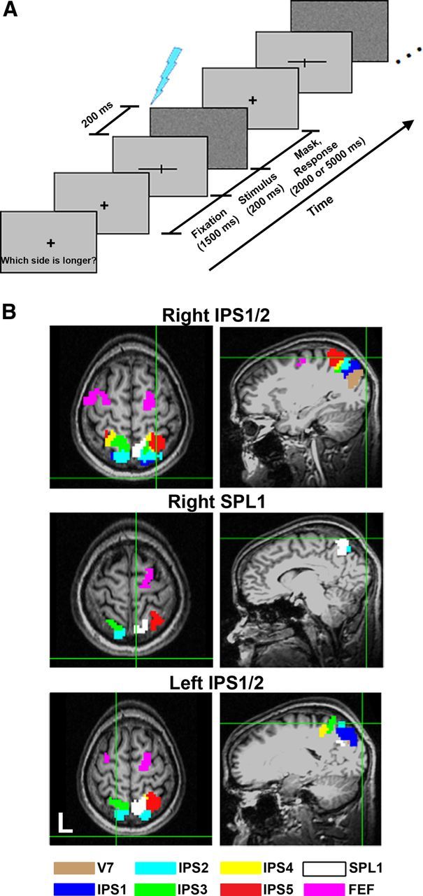
Landmark task and TMS target sites. A, Landmark task. Each block of the landmark task first began with instructions indicating whether subjects should judge which side of a horizontal line was longer or shorter. The same judgment was made for the entire block (example shows a “longer” block). Stimuli were horizontal lines shifted leftward or rightward in relation to a veridical midpoint defined by a vertical transection line. Note that the lines presented in the actual experiment were white, whereas the lines in this example are depicted as black for better contrast. Each trial started with a fixation point (displayed for 1500 ms), followed by a transected line stimulus (displayed for 200 ms), and ended with a full-screen mask (displayed for 2000 or 5000 ms during TMS). Subjects made their responses while the mask was displayed. During the TMS conditions, a single pulse (blue marker) was delivered over several ROIs (see below) at either 200 or 100 ms after the onset of the transected line stimulus during every trial. B, TMS target sites in PPC. Example in one subject (S3) of the three functional sites, right IPS1/2 (top row), right SPL1 (middle row), and left IPS1/2 (bottom row), that were targeted with TMS. Each topographic ROI is indicated by its own set of colored voxels. The green crosshairs indicate where the TMS coil was placed over each topographic area, as illustrated from a sagittal view (right column) and an axial view (left column).

A staircase procedure was used for determining the spatial bias, or the point of subject equality (PSE), in individual subjects. Each block began with horizontal line presentations that were shifted 1° of visual angle to either the left or the right of fixation, which was well above threshold for all subjects. Subjects were asked to make one of two judgments, “Which side is longer, right or left?” or “Which side is shorter, right or left?,” and stimuli were blocked according to their instruction (i.e., all “longer” judgments were made together and all “shorter” judgments were made together). Subjects were instructed to make a response on a keyboard using their right hand, specifically using their right index, middle, or ring finger to indicate the response (“left,” “neutral,” meaning that the two sides were perceived to be of equal length, or “right,” respectively). Stimuli were presented in a two-down, one-up manner, in which each horizontal line was presented twice at a certain distance shifted from fixation. If a subject responded correctly to both presentations of a stimulus with a certain offset, the horizontal line was then shifted closer to its bisection point by setting the new offset to 80% of the previous offset. The line was shifted away from its bisection point after one incorrect or one neutral response. The staircase procedure was run from both the right and the left, with trials coming from both sides randomly intermixed.

For each trial, a central fixation cross appeared for 1500 ms, followed by a transected line stimulus for 200 ms (a duration that prohibits eye movements). This was immediately followed by a full-screen mask of randomly presented black and white pixels that remained present for 2000 ms, during which time the subject responded. There were 80 trials per block and four blocks, or four complete staircase procedures, per session (two blocks during which subjects made “longer” judgments and two blocks during which they made “shorter” judgments). Order of instructions was counterbalanced between subjects.

Neuroimaging task, data acquisition, and analyses.

Twelve of the 46 subjects who participated in the landmark task also participated in one session to define topographically organized regions of interest (ROIs) within frontoparietal cortex. Six topographic ROIs in PPC (IPS1–IPS5 and SPL1) and two ROIs in frontal cortex [FEF, precentral cortex/inferior frontal sulcus (PreCC/IFS)] were defined in each hemisphere using a memory-guided saccade task (for details of the scanning parameters, behavioral task, and data analyses, see Kastner et al., 2007; Konen and Kastner, 2008). These topographically organized areas are known to overlap heavily with the dorsal frontoparietal spatial attention network (Szczepanski et al., 2010).

All 12 subjects also participated in an fMRI scanning session during which they performed a spatial attention task that was designed to determine the individual attentional weights for each of the topographically defined areas. Subjects were instructed to covertly attend to colorful, complex images presented peripherally to either the RVF or the LVF and to detect a target image (Szczepanski et al., 2010). A quantitative analysis of the time series of fMRI signals obtained in the spatial attention task was performed for each of the previously defined topographic ROIs in the LH and RH in each subject. The raw fMRI signals were extracted from the motion-corrected and undistorted echo planar images. Linear, mean, and quadratic trends were removed from the time series, and the signals were then averaged across all voxels activated by the spatial attention task (yielded by the contrast attended vs unattended, thresholded at an F score of 10.80, p < .001, uncorrected for multiple comparisons), within a given topographic ROI. fMRI signals for a given experimental condition (i.e., “Attend RVF” or “Attend LVF”) were normalized to the mean intensity of the four time points preceding the particular condition to yield percentage signal change. Mean signal changes were then derived for each of the conditions by averaging the eight peak intensities of the fMRI time series obtained in a given condition. A lateralization index (LI; Szczepanski et al., 2010) was then defined for each of the left and right ROIs to assess the degree to which the fMRI attention signals in each subject showed a preference for contralateral or ipsilateral presentations [LI = (R_contra − R_ipsi)/(R_contra + R_ipsi), in which R is response as mean signal change, contra is attention to contralateral presentations, and ipsi is attention to ipsilateral presentations]. Positive values indicate stronger responses to contralateral than ipsilateral presentations; negative values indicate the opposite. We previously proposed that the LI value for each of these LH and RH ROIs is an index of how much an area contributes to the control of spatial attention across the visual field by generating a spatial bias, or attentional weight, toward the contralateral hemifield (Szczepanski et al., 2010). The sum of the weights contributed by each area within a hemisphere constitutes the overall spatial bias that can be exerted over contralateral space. To examine this further, LI values were averaged across subjects and/or ROIs to yield group data. Statistical significance was assessed using repeated-measures ANOVAs and paired t tests (for additional details on the scanning parameters, behavioral task, and data analyses for the spatial attention data, see Szczepanski et al., 2010).

TMS task and procedure

Landmark task with TMS.

We used the modified version of the landmark task (Milner et al., 1992; Bjoertomt et al., 2002; Fig. 1A) described above to assess the behavioral spatial bias of each of our six TMS subjects. The stimuli were identical to those described above in the purely behavioral experiment, with a few exceptions. After stimulus presentation, a full-screen mask remained present for 5000 ms. The mask period, and thus the intertrial interval, was lengthened to allow recovery time for the TMS coil between discharges. Subjects completed 42 trials per block and four blocks for each session. The number of trials per block was shortened because of coil constraints; the coil heats up and automatically deactivates after too many consecutive discharges. A staircase procedure was again used, and blocks began with horizontal line presentations that were shifted 0.85° of visual angle to either the left or the right of fixation (again, high above threshold for all subjects), and with each pair of correct answers, the horizontal line was shifted closer to its veridical midpoint by setting the new offset to 70% of the previous offset. These changes were made because of the shortened number of trials per block, so that fewer trials would be needed for subjects to reach the PSE. Subjects performed six sessions of the landmark task: five sessions with TMS, which was applied to three different cortical sites and using two different stimulus onset asynchronies between stimulus presentation and pulse, and one purely behavioral session (“no-TMS” condition).

TMS.

Single-pulse TMS was delivered by a Magstim 200 monophasic magnetic stimulator at 60% of maximal stimulator output. This stimulation intensity was chosen because it was greater than the motor threshold in all subjects and several previous studies have found attention effects over both PPC and the FEF using the same intensity (Hilgetag et al., 2001; Ro et al., 2002; Muggleton et al., 2003; Ellison et al., 2004; O'Shea et al., 2004; Dambeck et al., 2006). We did not relate intensity to motor threshold because previous studies have shown that motor threshold cannot be assumed to guide excitability in distinct cortical areas (Stewart et al., 2001). Stimulation was delivered using a 70 mm figure-of-eight coil.

Before the TMS sessions, topographic ROIs in frontoparietal cortex (IPS1–IPS5, SPL1, FEF, PreCC/IFS) were identified using fMRI while subjects performed a memory-guided saccade task (Kastner et al., 2007; Konen and Kastner, 2008; Szczepanski et al., 2010). The topographic ROIs were overlaid on a corresponding T1-weighted anatomical MR image for each subject. Once these areas were defined in each of our subjects, we were able to use frameless stereotaxy (Brainsight; Rogue Research) in conjunction with a Polaris infrared positioning system (Northern Digital) to target specific functional areas for TMS. Three TMS sessions were conducted with the coil placed over three distinct regions of PPC: right IPS1/2, right SPL1, and left IPS1/2 [Fig. 1B illustrates the coil placement over each of these areas in an example subject (S3); mean Talairach coordinates (Talairach and Tournoux, 1988) for each of these topographic areas are given in Table 1]. We chose to interfere with these areas of the network because they are located close to the skull surface, thus making it feasible to target them with TMS. Several other areas, such as IPS3–IPS5, cannot be easily targeted with TMS, because these areas are often buried deep within the IPS. Because TMS of the FEF can induce facial and/or neck twitches (Goonetilleke et al., 2011), we targeted IPS areas only.

Table 1.

Talairach coordinates of topographic areas targeted for TMS stimulation

Area	x	y	z	n
IPS1
L	−24 (3.1)	−76 (1.2)	+41 (2.1)	6
R	+22 (2.7)	−74 (1.8)	+36 (2.8)	6
IPS2
L	−18 (2.8)	−69 (2.0)	+48 (3.1)	6
R	+17 (2.5)	−70 (1.8)	+47 (2.4)	6
SPL1
R	+7 (1.4)	−61 (4.7)	+50 (3.9)	6

Values are means ± SEM of peak coordinates in millimeters. n, Number of subjects showing significant clusters of activation; L, left; R, right.

A fourth “double TMS” session was conducted during which TMS pulses were administered to two of these areas simultaneously, with one coil placed over right IPS1/2 and one coil over left IPS1/2. The coil was always placed tangentially to the skull with the handle of the coil parallel to the midsagittal plane, except in the double TMS condition, in which the handle of each coil was turned slightly more perpendicular to the midsagittal plane to fit both coils on the head at once. For each of these sessions, a single pulse was delivered 200 ms after the onset of the transected line stimulus during every trial (Fig. 1A). This timing was chosen based on previous electroencephalography (EEG) studies that suggest that visual spatial attention enhances the amplitude of the N1 component of the event-related potential (ERP) ∼180–200 ms after stimulus (Makeig et al., 1999; Vazquez Marrufo et al., 2001). In a fifth session, TMS over right SPL1 was also delivered 100 ms after stimulus onset as a timing control. Because an audible click was generated with each pulse, subjects wore earplugs during each session.

Data analyses

Landmark task.

Trials from each block were organized into bins based on their distance from the veridical midpoint. These bin boundaries were placed 0.1° of visual angle apart. The proportion reported as “right is longer” was then calculated for the set of trials that fell into a bin for a single block. Subjects' responses were reversed for “Which is shorter?” trials (i.e., “left is shorter” is equivalent to “right is longer”). Each of these data points across blocks was plotted on the same graph. The offset of the horizontal line to the left or the right was plotted (x-axis) against the proportion of trials reported as “right is longer” (y-axis). A Weibull function was then fit to the data to estimate a psychometric function (for an example, see Fig. 3A). We calculated each individual subject's behavioral spatial bias by finding the point on the Weibull function in degrees of visual angle that corresponded to when left and right were reported equally often (i.e., the PSE; see Fig. 3A, gray lines).

Figure 3.

Behavioral spatial biases. A, Examples of spatial biases obtained in two subjects (S12, left; S2, right) using the landmark task. Trials from each block were organized into bins based on their distance from the veridical midpoint (marked by the dashed line in each graph). The proportion reported as “right is longer” was then calculated for the set of trials that fell into a bin for a single block (thus, each × represents data from a single bin from 1 of the 4 blocks). The offset of the horizontal line to the left or the right was plotted against the proportion of trials reported as “right is longer,” and the data were fit with a Weibull function (A, black curves). Each individual subject's behavioral spatial bias was the point on the function in degrees of visual angle that corresponded to when left and right were reported equally often (i.e., the PSE; A, gray lines). Left, An example of a subject (S12) with a leftward behavioral bias (PSE is to the left of the veridical midpoint). Right, An example of a subject (S2) with a rightward behavioral bias (PSE is to the right of the veridical midpoint). B, Distribution of behavioral biases across all subjects tested in the landmark task (n = 45). The histogram represents the number of subjects with a given bias to the right (RVF bias) or the left (LVF bias) of the veridical midpoint (represented by the dotted line). For a subset of these subjects (n = 12), the behavioral bias values were correlated with their respective neural spatial bias (LI) values. The distribution of behavioral spatial bias values for these 12 subjects is shown in gray.

Correlation between behavioral spatial bias and neural bias.

We examined the relationship between the average neural bias (average LI value) across all topographic areas and the behavioral spatial bias as measured with the landmark task in each of the 12 fMRI subjects. We reasoned that, if all of the topographic areas respond to spatial attention, they might all contribute toward the overall behavioral spatial bias observed in individual subjects, and the average LI value across all ROIs in both hemispheres might therefore be the best predictor of any behavioral bias. LI values in the RH were given a positive sign, whereas the LI values in the LH were given a negative sign, so when they were averaged across hemispheres, subjects with an overall stronger neural bias in the LH had negative LI values and those with an overall stronger neural bias in the RH had positive LI values. All values were then standardized to z-scores. Pearson's product-moment correlations were calculated between the average LI values across all topographic ROIs and both dependent measures (the behavioral spatial bias scores from the landmark task and the Edinburgh Handedness Inventory scores). In addition, Pearson's product-moment correlations were also calculated between the LI values for each individual topographic area (averaged across hemispheres) and behavioral spatial bias scores to determine which individual areas might best predict the behavioral spatial bias. Correlations were also calculated between each individual area and handedness scores. To control for multiple comparisons, the p values from the correlation analyses were then corrected using the false discovery rate procedure outlined by Benjamini and Hochberg (1995). The resulting corrected p values were considered significant at p = 0.05.

TMS.

Behavioral data were analyzed as described above for the landmark task. For each subject, the data for the five TMS sessions (right IPS1/2–200 ms, right SPL1–200 ms, right SPL1–100 ms, left IPS1/2–200 ms, and simultaneous left and right IPS1/2–200 ms) and the no-TMS session were each fit with a Weibull function, and the PSE/behavioral spatial bias was calculated (for an example, see Fig. 5). Thus, we calculated six behavioral spatial bias values for each subject, each corresponding to a different condition/TMS session. Behavioral biases were then averaged across all subjects for each condition. The average value of the no-TMS condition was then added to the average value of each condition, such that the no-TMS condition was set to zero, serving as a baseline, whereas the remaining conditions were expressed as an offset in degrees of visual angle from the baseline condition. Paired t tests were used to determine whether there were systematic shifts in the behavioral spatial bias between the no-TMS condition and each of the TMS conditions across subjects. Note that the no-TMS condition was not the only control condition. Each of the five TMS sessions served as a control condition for the other four sessions, with right SPL1–100 ms and simultaneous left and right IPS1/2–200 ms serving as the most critical control conditions.

Figure 5.

Behavioral spatial biases of individual subjects for each TMS condition. Examples of Weibull functions derived from data collected from four of the six subjects who underwent TMS while performing the landmark task. Each curve represents the data collected from a separate TMS condition (red curves, data from right SPL1 stimulation; blue curves, data from right IPS1/2 stimulation; green curves, data from left IPS1/2 stimulation; cyan curves, data from simultaneous left and right IPS1/2 stimulation). Each of the TMS conditions was compared with the data collected while subjects performed the landmark task without TMS (no-TMS condition; black curves). Solid curves represent data collected while TMS was applied 200 ms after stimulus onset, and the dashed curves represent data collected while TMS was applied 100 ms after stimulus onset. The vertical, solid black lines indicate the PSE/ behavioral spatial bias for each condition. All other conventions are as in Figure 3A.

Results

Individual differences in neural spatial bias

As reported previously, the dorsal frontoparietal attention network can be subdivided into at least 16 different areas based on their topographic organization (Kastner et al., 2007; Konen and Kastner, 2008; Szczepanski et al., 2010). These topographic areas include IPS1–IPS5 and SPL1 in PPC, as well as the putative human FEF in superior, lateral PreCC, and the putative human SEF in dorsal medial frontal cortex. We previously examined the spatial attention signals separately in each of these topographic areas while subjects performed a sustained attention task in which they were instructed by a brief occurrence of a cue at fixation to covertly direct attention to either the RVF or LVF and to count the occurrences of a target stimulus that appeared in the periphery (Szczepanski et al., 2010). Figure 2A shows an example of the activations obtained when a representative subject directed attention to the periphery while performing this attention task, relative to attending to a central location (p < 0.001), with the subject's topographic areas indicated by the black outlines. In each topographic area, responses to attended stimuli in the contralateral hemifield were stronger than those to attended stimuli in the ipsilateral hemifield. To quantify these spatial attention biases, we defined an LI for each individual ROI, which indicated how strongly an area responded to the contralateral versus ipsilateral side of space (for definition, see Materials and Methods). Figure 2A depicts the LI value for each topographic area averaged across the group of subjects (n = 12). All LI values were positive, indicating that each area responded more strongly when attention was directed toward the contralateral than to the ipsilateral side of space. Based on these results, we propose that each of the topographic areas contributes toward the control of spatial attention across the visual field by generating a spatial bias, or an attentional weight, toward the contralateral side of space, as indexed by its LI value. We consistently observed several asymmetries within this network across the group of subjects: left FEF, IPS1, and IPS2 exerted stronger attentional weights than their RH counterparts, whereas right SPL1 contributed a strong attentional weight toward the LVF but did not appear to have an LH counterpart (Szczepanski et al., 2010). Importantly, these right and left asymmetries were approximately balanced out across the entire network, supporting the idea that all areas of the frontoparietal network contribute to the control to spatial attention rather than only a few areas in particular. However, it should be noted that this interhemispheric competition account currently only considers the cortical network and, as a result of a lack of data, does not yet include subcortical areas, such as the superior colliculus (SC) and the pulvinar, which are known to play an important role in visual attention (Saalmann et al., 2012; Zénon and Krauzlis, 2012).

Figure 2.

Spatial attention signals across human frontoparietal cortex. A, The neural bias toward the RVF or LVF, as assessed by an LI, for each individual topographic ROI averaged across the group of subjects (n = 12). Example of activations within frontal (top) and parietal (bottom) cortices projected onto an inflated surface of a representative subject's brain. Topographically organized ROIs are outlined in black. Numbers represent the average LI value for each topographic ROI. B, The LI values averaged across all ROIs within the LH and RH across subjects. Across the group, the average LI was not significantly different between hemispheres. Error bars indicate SEM. N.S., Not significant. C, The LI values averaged across all of the RH ROIs (x-axis) plotted against the LI values averaged across all of the LH ROIs (y-axis) for each individual subject (n = 12). There was a large amount of intersubject variability in LI values between hemispheres. Dashed line represents the equality line.

The LI values averaged across all topographic areas within a hemisphere did not differ significantly between the LH and the RH across the group (p > 0.40; Fig. 2B). In other words, the spatial attention bias between the two hemispheres appeared to be balanced, such that together the areas in each hemisphere seemed to control attention equally toward the contralateral side of space. However, when we examined the LI values of individual subjects, we found a considerable amount of intersubject variability (Fig. 2C). When the LI values averaged across all of the RH ROIs were plotted against the LI values averaged across all of the LH ROIs for each individual subject who participated in the fMRI study, it was apparent that some subjects had stronger spatial attention biases in their RH areas (below the dashed equality line), some had stronger biases in their LH areas (above equality line), and a few had relatively equal biases between the two hemispheres (along the equality line) (Fig. 2C). Thus, the hemisphere with the stronger contralateral attention signals was highly individualized.

Individual differences in behavioral spatial bias

We next investigated whether the individual differences in spatial attention bias that we observed at the neural level were also reflected at the behavioral level. We assessed behavioral spatial bias using the landmark task (Milner et al., 1992; Bjoertomt et al., 2002; Fig. 1A), which requires subjects to make judgments about whether pretransected lines are longer to the left or right of a vertical transection point. We chose to use the landmark task because it is the perceptual version of the line bisection task, which has long been considered an effective clinical approach to evaluate spatial bias in patients with suspected visual neglect (Axenfeld, 1915). During the line bisection task, patients are presented with a horizontal line and are asked to draw a vertical bisection through it. Neglect patients bisect the line far to the right of the veridical midpoint, suggesting that their attentional bias has shifted toward the RVF (Schenkenberg et al., 1980; Bisiach et al., 1983). The landmark task is often used to assess behavioral spatial bias in healthy subjects instead of the line bisection task, because it does not require a motor response (Milner et al., 1992; McCourt and Olafson, 1997; McCourt and Jewell, 1999). A modified version of the landmark task, in which trials were staircased, was used for the current study (Fig. 1A; see Materials and Methods). Some individual subjects had leftward behavioral spatial bias values (for example, S12; Fig. 3A, left) and some had rightward values (for example, S2; Fig. 3A, right) while performing the landmark task.

The behavioral spatial bias was initially computed for 46 subjects using the landmark task to determine the distribution of bias values within a larger population of subjects. We found a considerable amount of variability in the behavioral spatial bias across individual subjects (Fig. 3B), with the biases of some subjects located far to the right (13.04% of subjects had biases that were 1 SD above the mean), some far to the left (15.22% of subjects had biases that were 1 SD below the mean), and a majority located close to the veridical midpoint (71.74% of biases were within 1 SD to the right or the left of the mean). The average bias across all 46 subjects was located slightly to the right of the veridical midpoint (0.02 ± 0.03° of visual angle). The average behavioral spatial bias across the group of 12 subjects who also participated in the fMRI scanning (0.06 ± 0.04° of visual angle) was located slightly farther to the right than that of the larger group (gray histogram in Fig. 3B depicts the distribution of behavioral spatial bias values for the fMRI subjects).

Many past studies investigating behavioral spatial biases using the landmark task have reported an average leftward bias across a group of subjects (Milner et al., 1992; McCourt and Olafson, 1997; McCourt and Jewell, 1999). This leftward bias has been termed “pseudoneglect,” or “left-side underestimation,” and has been traditionally associated with a right hemispheric dominance for spatial attention (Bowers and Heilman, 1980). However, the group of subjects for the current study had an average rightward bias (and the total number of subjects exhibiting a rightward bias was larger than the number exhibiting a leftward bias; Fig. 3B). Our results are not necessarily atypical. Although leftward pseudoneglect has been reported in several studies (Bisiach et al., 1976; Heilman et al., 1985; Scarisbrick et al., 1987; Werth and Pöppel, 1988), there are some studies that have found a rightward bias in a group of normal subjects (Schenkenberg et al., 1980; Manning et al., 1990; Butter and Kirsch, 1992). In fact, a number of studies have noted substantial individual differences in landmark task performance among subjects (Bowers and Heilman, 1980; Halligan et al., 1990; Manning et al., 1990; McCourt and Olafson, 1997; Cowie and Hamill, 1998). Thus, a particular sample of subjects can strongly influence group results. This suggests that an individual-subject analysis approach, such as the one taken in the current study, rather than a group average approach, may be more sensitive when examining spatial attention behavior.

Relationship between neural and behavioral spatial biases

The relationship between the strength of the spatial biasing signals across frontoparietal topographic areas and the resulting behavioral spatial bias was next investigated by plotting a single LI value, calculated by averaging the individual LI values across all topographic ROIs, against the corresponding behavioral bias score, as indexed by the landmark task, for each subject. We found a strong negative relationship between the behavioral spatial bias and the LI value averaged across all topographically organized areas (r₍₁₀₎ = −0.71, p < 0.05, corrected, SEM = 0.22; Fig. 4). In other words, subjects with stronger LI values on average in the LH tended to show a bias toward the RVF while performing the landmark task, and those with stronger LI values on average in the RH tended to show a bias toward the LVF while performing the landmark task. Therefore, it appears that the neural spatial bias averaged across both hemispheres of the entire frontoparietal attention network can be used to predict whether an individual subject's behavioral spatial bias falls toward the RVF or LVF. Based on these results, we propose that competition between spatial biasing signals produced by the frontoparietal areas in each hemisphere is what determines behavioral spatial bias. For example, if the neural spatial bias in an individual is stronger in one hemisphere than the other, it will produce a stronger attentional weight toward the contralateral visual field, resulting in a behavioral bias toward that visual field. Subjects with unequal neural biases between hemispheres will exhibit skewed behavioral biases, whereas subjects with relatively equal neural biases between hemispheres will exhibit behavioral biases that are less skewed.

Figure 4.

Relationship between behavioral bias and neural bias. For each subject (n = 12), the behavioral spatial bias value (in degrees of visual angle), calculated using the landmark task, was plotted against the neural bias value (the average LI value across all topographically organized areas in parietal and frontal cortices), calculated from data gathered in a separate fMRI spatial attention experiment. The dotted line represents the regression line through the data. Subjects with stronger neural biases on average in the LH tended to show a bias toward the RVF while performing the landmark task, whereas those with stronger neural biases on average in the RH tended to show a bias toward the LVF while performing the landmark task.

It is possible that some areas within the frontoparietal network contributed to the behavioral spatial bias more than others. To investigate this, we calculated the correlations between behavioral spatial bias values and the LI values for each individual area (averaged across hemispheres). Only the LI values of IPS5 correlated significantly with behavioral spatial bias values (r₍₁₀₎ = −0.70, p < 0.05, corrected, SEM = 0.13), whereas the LI values from the other individual areas did not (p values > 0.05, corrected). Individually, neither IPS1 nor IPS2 correlated significantly with behavior. However, when the two areas were averaged together (right IPS1, right IPS2, left IPS1, left IPS2), the resulting LI values correlated significantly with behavior (r₍₁₀₎ = −0.81, p < 0.02, corrected, SEM = 0.10).

We were additionally interested in the relationship between the degree of handedness, as measured by the Edinburgh Handedness Inventory (Oldfield, 1971), and the degree of spatial attention bias in frontoparietal topographic areas. The degree of handedness did not predict the average LI value across all topographic areas (r₍₁₀₎ = −0.26, p > 0.60, corrected, SEM = 0.30). The degree of handedness also did not predict any of the LI values from individual topographic ROIs (p values > 0.40, corrected). Thus, the degree of laterality of spatial attention signals in frontoparietal cortex appears to be unrelated to the degree of handedness.

The above analyses established a correlational relationship between neural biasing signals in areas of frontoparietal cortex and behavior in the landmark task. We next wanted to study the impact of an individual area on the overall neural, and thus behavioral, bias within the system. To do this, we used TMS to establish a causal relationship between the neural signals produced by individual areas of the dorsal frontoparietal attention network and changes in behavioral spatial bias.

Testing the contributions of individual areas to the overall behavioral spatial bias

To test our predictions further in a more causal manner, we used single-pulse TMS, in conjunction with frameless stereotaxy and fMRI-guided coil placement, to interfere with attentional processing in individual nodes of the dorsal frontoparietal attention network in a subset of our fMRI subjects (n = 6) while they performed the landmark task (Fig. 1A; as described above, with a few modifications; see Materials and Methods). We hypothesized that transient interference of one or more areas of the dorsal attention network areas should produce a temporary shift of the residual attentional weights within the system, resulting in a reallocation of spatial attention toward the visual field ipsilateral to the stimulation. For example, TMS over right frontoparietal cortex should disrupt some weights that control attention toward the LVF, leading to a stronger spatial bias toward the RVF when performing the landmark task, whereas TMS over left frontoparietal cortex should disrupt some weights that control attention toward the RVF, leading to a stronger spatial bias toward the LVF when performing the landmark task.

We initially chose to interfere with two individual locations in PPC: right IPS1/2 and left IPS1/2 (for an example of each target location in a representative subject, see Fig. 1B). These areas were chosen because the averaged IPS1/2 LI values correlated well with behavioral spatial bias values. For each of these conditions, TMS was applied at 200 ms after each stimulus onset while subjects performed the landmark task. Behavioral data collected while subjects performed the landmark task in the absence of TMS (no-TMS condition; Figs. 5, black lines, 6, black circle) were used to define each subject's initial behavioral spatial bias and served as an anchor from which to compare all other conditions. These initial spatial biases differed greatly between subjects (Fig. 5). One subject had an initial bias to the right (Fig. 5, S4), whereas the rest had initial biases to the left. TMS applied to right IPS1/2 at 200 ms after stimulus onset induced a significant rightward shift of the average behavioral spatial bias [0.11 ± 0.07° visual angle (mean ± SEM); Fig. 6, blue triangle] compared with the average behavioral bias without TMS (0.0 ± 0.07° visual angle) (t₍₅₎ = 2.93, p < 0.05). This effect was observed as a rightward shift of the Weibull function for every individual subject (Fig. 5, blue solid lines) compared with the no-TMS condition. The opposite pattern was found when TMS was applied at 200 ms after stimulus onset over left IPS1/2: behavioral bias values were shifted leftward (−0.14 ± 0.09° visual angle; Fig. 6, green triangle) compared with bias values without TMS (t₍₅₎ = 3.06, p < 0.05). This effect was also observed as a leftward shift of the Weibull function for every individual subject compared with the no-TMS condition (Fig. 5, green lines).

Figure 6.

Behavioral spatial biases for each TMS condition averaged across subjects. The average behavioral spatial bias (in degrees of visual angle) across subjects (n = 6) for each TMS condition (red points, TMS over right SPL1; blue point, TMS over right IPS1/2; green point, TMS over left IPS1/2; cyan point, TMS over left and right IPS1/2) compared with the average behavioral spatial bias across subjects when TMS was not applied (no-TMS condition; black circle). Triangles indicate conditions during which TMS was applied 200 ms after stimulus onset. Diamond indicates the condition during which TMS was applied 100 ms after stimulus onset. *p < 0.05; **p < 0.01; N.S., not significant. Error bars indicate SEM.

To determine whether or not each individual topographic area of the dorsal frontoparietal attention network contributes toward the overall spatial bias that is generated by the network, we applied TMS using the same timing parameters to a third PPC area, right SPL1, which did not correlate so well with behavior (r₍₉₎ = −0.38, p > 0.30, corrected, SEM = 0.17). TMS applied to right SPL1 at 200 ms after stimulus onset (0.13 ± 0.06° visual angle; Figs. 5, red solid lines, 6, red triangle) induced a significant rightward shift in subjects' bias values compared with the no-TMS condition (t₍₅₎ = 4.38, p < 0.01). To examine the temporal specificity of these effects, subjects also performed the landmark task while TMS was applied to right SPL1 at 100 ms after stimulus onset. There were no significant differences between behavioral bias values when TMS was applied 100 ms after stimulus onset over right SPL1 (0.03 ± 0.07° visual angle; Figs. 5, red dashed lines, 6, red diamond) and behavioral bias values produced without TMS (t₍₅₎ = 1.90, p > 0.10). However, TMS at 200 ms after stimulus onset induced a significant rightward shift in subject's bias values compared with TMS at 100 ms after stimulus onset (t₍₅₎ = 2.85, p < 0.05). It therefore appears that the induced effects are fairly temporally specific, which is consistent with previous studies that have demonstrated visual attentional effects at a latency of ∼180–200 ms after stimulus onset (Makeig et al., 1999; Vazquez Marrufo et al., 2001).

The 100 ms TMS condition over SPL1 also serves as an important control, because it demonstrates that stimulation of the identical cortical site while using nearly identical environmental settings does not always result in a significant behavioral change. Although attentional orienting takes longer in the visual modality, attentional orienting in the auditory modality occurs much more quickly. In EEG studies, the first ERP wave that is modulated by attention using auditory stimuli, the auditory N1, peaks between 80 and 120 ms (Hillyard et al., 1973; Schwent and Hillyard, 1975). Therefore, the 100 ms TMS condition is an appropriate control for any orienting effects that may potentially occur attributable to the auditory clicking sound. In fact, if the 100 ms TMS condition had produced a significant shift in behavioral spatial bias, it would suggest that we were manipulating auditory attention rather than visual attention. Our results indicate that the 100 ms TMS condition did not differ significantly from the no-TMS condition across subjects. Thus, the 100 ms TMS condition appears to serve as an appropriate control for (1) the significant visual attentional effects that occur later in time because it demonstrates that these observed effects are temporally specific and (2) the auditory attentional effects that could potentially occur if subjects were orienting to the clicking sound made by the TMS machine, which does not appear to be the case.

The most critical prediction from the interhemispheric competition account is that simultaneous disruption of both right and left areas of the network should affect attentional weights approximately equally, thereby resulting in an overall balance of the neural spatial bias across hemispheres and therefore no net change in behavioral bias. This was tested in a condition during which single-pulse TMS was administered simultaneously to both right and left IPS1/2 at 200 ms after stimulus onset. The behavioral bias (−0.05 ± 0.10° visual angle; Fig. 6, cyan triangle) produced by simultaneous TMS was not significantly different from the behavioral bias produced without TMS (t₍₅₎ = 1.21, p > 0.20). In addition, TMS applied individually to left or right IPS1/2 shifted behavioral bias values significantly leftward (t₍₅₎ = 6.62, p < 0.001) or rightward (t₍₅₎ = 2.67, p < 0.05), respectively, compared with the simultaneous TMS condition. These results are also reflected in the data for each individual subject (Fig. 5, cyan lines). This suggests that disruption of both IPS1/2 areas in opposite hemispheres effectively cancels out any effects produced by disruption of either area alone.

One possible concern is that disruption of right SPL1 and right IPS1/2 produced similar behavioral effects because of their close proximity. That is, because TMS may not have a fine enough spatial resolution to differentiate between the two areas, both areas could have been disrupted together. Indeed, the two regions are adjacent to each other in the subject provided as an example (Fig. 1B). However, this is not the case in every subject. For example, right SPL1 is separated from right IPS1 and right IPS2 by >15 mm (1.5–2.5 cm) in all directions in S1, S4, S5, and S6. Across the group of subjects, the mean Talairach coordinates for right SPL1 are 12.3 ± 1.5, 11.2 ± 5.7, and 8.7 ± 3.6 mm (mean ± SEM in the x, y, and z directions, respectively) apart from the mean Talairach coordinates for right IPS1/2 (coordinates for right IPS1/2 were defined as the average of the IPS1 and IPS2 coordinates; see Table 1). In the visual system, phosphene mapping has suggested a spatial resolution of ∼1 cm or less when TMS is applied over the occipital pole (Kammer, 1999). However, this spatial resolution depends on the exact stimulation parameters used (i.e., the shape and orientation of the coil, the intensity of the TMS pulse, and the underlying brain anatomy), so we cannot be certain of the exact spatial resolution for this particular TMS experiment. However, right SPL1 and right IPS1/2 were located on average more than (or exactly) 1 cm apart from each other in all directions, and in several subjects, the two areas were located much farther apart than 1 cm. Therefore, it seems unlikely that TMS over right SPL1 caused disruption of right IPS1/2 and vice versa across all subjects.

In summary, TMS over each individual PPC area shifted behavioral spatial biases ipsilaterally in each subject, whereas simultaneous TMS over right and left IPS1/2 produced biases that were no different from subjects' biases under baseline conditions. Therefore, TMS interference over both IPS sites simultaneously can “correct” the bias that is produced by TMS to just one site alone. This demonstrates that each targeted topographic area in PPC made its own significant contribution toward the overall spatial bias exerted over the visual field. Furthermore, these data support the overarching hypothesis that the spatial signals from these topographic areas combine to produce an overall neural bias across the system that determines the attentional behavior of individual subjects. These data are consistent with an interhemispheric competition account of spatial attention control, in which each hemisphere directs attention toward the contralateral visual field and is balanced through reciprocal inhibition (Kinsbourne, 1977, 1993; Cohen et al., 1994).

We cannot indisputably argue that all frontal and parietal areas contribute an attentional weight toward contralateral space based on the evidence presented in this study. Such an argument would require disruption of every individual area with TMS. However, this is not feasible, because some areas are inaccessible using the TMS method (e.g., cortical areas buried in deeper parts of the IPS as well as subcortical areas). We therefore reasoned that all areas contribute to the control of attention across contralateral space based on three arguments; (1) the correlation between behavioral spatial bias values and the LI values averaged across all frontoparietal areas is still larger than the correlation between behavior and any individual area; (2) even areas that do not correlate well with individual behavioral spatial bias values, such as SPL1, appear to contribute to the control of contralateral space (i.e., TMS to SPL1 shifted behavioral spatial biases); and (3) the hemispheric asymmetries across different areas of the network suggest that the entire network is needed to balance attentional allocation across the visual field. Therefore, although the LI values from IPS5 as well as IPS1/2 combined correlate significantly with behavior, it appears that the activity from multiple areas across the network is what best determines behavior. Because several areas of the network identified in the fMRI study generate spatial biases but cannot be investigated using TMS, we think the most conservative approach to investigating this relationship between brain function and behavior is to consider the entire network rather than focusing only on areas that are easily targeted with TMS. For these reasons, we argue that it is important to focus on the network as a whole, rather than focusing on individual areas, when examining correlations with behavior.

Discussion

We used a multimodal experimental approach consisting of fMRI, topographic mapping, behavioral measures of spatial bias, and fMRI-guided single-pulse TMS to investigate the neural basis of spatial attentional control. Together, this multimodal approach, in combination with an emphasis on neural and behavioral individual differences, provides compelling evidence for an interhemispheric competition account of spatial attention control (Kinsbourne, 1977; Cohen et al., 1994; Smania et al., 1998) in the intact human brain.

Spatial attention control and interhemispheric competition

We found large variability in the relative strengths of the attentional weights between right and left frontoparietal areas across the group of fMRI subjects. This observed intersubject variability appeared to be functionally significant because the attentional weights of individual subjects could be used to predict their respective behavioral preference when allocating attention across the visual field, as measured by a staircased landmark task. This result suggests that the combination of spatial signals from all topographic areas across both hemispheres of the dorsal attention network determines an individual subject's behavioral bias. It also suggests that each topographic area within the network may make its own individual contribution toward the overall spatial bias exerted across the visual field. To investigate the contributions made by each of these areas to an individual subject's overall behavioral spatial bias, we used single-pulse TMS to systematically disrupt individual topographic areas within the dorsal attention network. TMS over each individual area (right IPS1/2, left IPS1/2, right SPL1) consistently shifted behavioral spatial biases toward the ipsilateral visual field in individual subjects and across the group.

These fMRI and TMS results provide strong support for an interhemispheric competition account of spatial attention control, in which each of the frontoparietal topographic areas in the RH and LH generates a spatial bias, or attentional weight, toward the contralateral hemifield. The sum of these weights within a hemisphere constitutes the overall spatial bias that can be exerted toward the contralateral visual field, with the weights in each hemisphere balanced through reciprocal inhibition (Kinsbourne, 1977, 1993; Cohen et al., 1994). The strongest support for this interhemispheric competition model was provided by the condition during which both hemispheres of PPC were disrupted. Simultaneous TMS to both right and left IPS1/2 resulted in no net change in behavioral bias across subjects, although TMS to each of those individual areas shifted biases ipsilaterally. The interhemispheric competition account outlined above would predict such a result, because interference in both hemispheres should maintain an approximate balance within the system. Our findings are the first to demonstrate a neural basis for interhemispheric competition of attentional control in the intact human brain (Seyal et al., 1995; see also Blankenburg et al., 2008) and complements previous studies that have provided evidence in support of interhemispheric competition in neglect patients (Oliveri et al., 1999; Corbetta et al., 2005; Shindo et al., 2006; Sparing et al., 2009).

Several neural mechanisms could mediate this hemispheric rivalry. One possibility is that competition between frontoparietal areas in the two hemispheres is mediated through direct corticocortical connections. PPC and frontal areas within each hemisphere are directly connected via the corpus callosum in the human (Hofer and Frahm, 2006), making this the fastest and most direct route for spatial attention control across the visual field. Alternatively, hemispheric rivalry could be mediated through cortical–subcortical connections. For example, Sprague (1966) demonstrated that hemianopia resulting from unilateral ablation of visual cortex could be reversed by removal of the contralesional SC or by splitting the collicular commissure. This suggests that, once the ipsilesional SC is no longer inhibited by the contralesional SC, the ipsilesional SC may return to function and mediate the recovery from hemianopia. Because several subcortical structures, including the SC, pulvinar, and lateral geniculate nucleus, are modulated by spatial attention in the human (O'Connor et al., 2002; Cotton and Smith, 2007; Schneider and Kastner, 2009), cortical–subcortical interactions may underlie the observed hemispheric rivalry. Furthermore, these subcortical areas may partly determine the behavioral spatial bias of individual subjects. The current study focuses on cortical areas only, because the attentional weights generated by subcortical structures are currently unknown and, more importantly, cannot be disrupted using TMS. Additional research is needed to determine the exact mechanisms through which interhemispheric competition occurs.

The current study has important clinical implications for patients suffering from visual neglect as a result of parietal lesions. Evidence from previous studies suggests that, after damage to frontoparietal cortex, the intact hemisphere attempts to compensate for the lesioned hemisphere by increasing its activity (Corbetta et al., 2005; Voytek et al., 2010). However, this compensatory process is often slow because neglect symptoms can last for months to years after damage. The interhemispheric competition account suggests that, if frontal regions, including the FEF, remain intact in the damaged hemisphere, then training these areas to evoke a stronger attentional weight toward the contralesional visual field could help to rebalance the system and to ameliorate neglect symptoms. This could be accomplished by training patients to exert more top-down control toward the contralesional field (Parton et al., 2004), by increasing the processing priority of stimuli by manipulating stimulus salience in the contralesional visual field (Bays et al., 2010), or in light of the present results, possibly by using TMS to repetitively stimulate the FEF or other frontal structures that are involved in attentional selection.

Brain–behavior correlations and individual differences

The current study provides some of the first evidence for a link between spatial attention signals in frontoparietal areas and individual differences in behavior. We found a strong brain–behavior correlation, such that an individual's behavioral spatial bias, as measured with the landmark task, can be predicted by the neural spatial bias averaged across both hemispheres of topographic frontoparietal cortex. We would not have reached this same conclusion had we averaged LI values (Fig. 2B) or behavioral bias values across subjects, which is the standard form of group analysis for most fMRI and behavioral studies. Rather, these results are revealed only if the brain–behavior relationship is examined on an individual-subject level. Our results suggest that the individual differences within a small sample of fMRI subjects are potentially important to note, because they can have a tremendous impact on what conclusions are drawn from a study.

The results of the current study are consistent with previous studies demonstrating that TMS over right inferior parietal lobule produces a rightward bias when subjects perform the landmark task (Fierro et al., 2000; Pourtois et al., 2001; Bjoertomt et al., 2002; Brighina et al., 2002). However, all of these studies either chose not to examine the left PPC or failed to find significant results after LH stimulation, which has typically been interpreted as support for the hemispatial attention theory (Heilman and Van Den Abell, 1980; Mesulam, 1981). In comparison, the current study finds no evidence for RH dominance of spatial attention control. Instead, it provides evidence that TMS over left IPS1/2 shifts behavioral spatial biases leftward, which is more consistent with an interhemispheric competition theory of attention (Capotosto et al., 2012). The discrepancy in findings between the current study and many previous TMS studies is likely related to our analysis approach. Previous studies have determined parietal locations for stimulation using either scalp positions from the international standardized 10/20 EEG system (Pourtois et al., 2001; Brighina et al., 2002) or anatomical landmarks in combination with frameless stereotaxy (Bjoertomt et al., 2002). However, these localization methods do not account for intersubject functional and/or anatomical variation and therefore result in spatial imprecision. In particular, the inconsistent results produced by right versus left PPC TMS could be explained by greater anatomical variability in left PPC as a result of lateralized representations of human-specific abilities (Nelson et al., 2010). We chose to use a detailed ROI-based functional mapping technique that carefully considered individual differences in functional and anatomical neuroanatomy by identifying numerous frontoparietal topographic areas within each subject. When used in conjunction with frameless stereotaxy, this approach allowed precise targeting of particular functional areas with TMS to test specific hypotheses on an individual-subject level.

Unlike several other studies that correlate behavior with attention signals in visual and frontoparietal cortex (Sylvester et al., 2007, 2009), subjects in the current study performed a behavioral task that was unrelated to the task used in the fMRI portion of the study. Therefore, the neural asymmetries defined with one task (i.e., attending to peripheral stimuli presented in either the RVF or LVF) translate to behavioral asymmetries in a completely different task (i.e., the landmark task). This is important because it suggests that the attentional weights observed for each fMRI subject predict individual behavioral biases in a more general (i.e., task-independent) manner.

Our results also suggest that the individual differences observed among subjects are functionally meaningful (i.e., the differences in attentional weights reflect how individuals allocate attention across the visual field). This is especially important to consider when dealing with individuals who have sustained damage to portions of the frontoparietal attention network and may be suffering from various attentional deficits, including visuospatial neglect. Visuospatial neglect is a multifaceted disorder with highly variable symptoms among patients. To gain a full understanding and to develop treatment options for individual patients afflicted with neglect or other attentional disorders, it is necessary to examine the neural basis of individual differences in spatial attention control in the intact human brain. The current study is a first step to such an understanding.

References

- Anderson B. Pieces of the true crossover effect in neglect. Neurology. 1997;49:809–812. doi: 10.1212/wnl.49.3.809. [DOI] [PubMed] [Google Scholar]
- Axenfeld T. Hemianopische gesichtsfeldstorungen nach schadelschussen. Klin Monatsbl Augenheilkd. 1915;55:126–143. [Google Scholar]
- Bays PM, Singh-Curry V, Gorgoraptis N, Driver J, Husain M. Integration of goal- and stimulus-related visual signals revealed by damage to human parietal cortex. J Neurosci. 2010;30:5968–5978. doi: 10.1523/JNEUROSCI.0997-10.2010. [DOI] [PMC free article] [PubMed] [Google Scholar]
- Benjamini Y, Hochberg Y. Controlling the false discovery rate: a practical approach to multiple testing. J R Stat Soc Ser B Stat Methodol. 1995;57:289–300. [Google Scholar]
- Bisiach E, Capitani E, Colombo A, Spinnler H. Halving a horizontal segment: a study on hemisphere-damaged patients with cerebral focal lesions. Schweiz Arch Neurol Neurochir Psychiatr. 1976;118:199–206. [PubMed] [Google Scholar]
- Bisiach E, Bulgarelli C, Sterzi R, Vallar G. Line bisection and cognitive plasticity of unilateral neglect of space. Brain Cogn. 1983;2:32–38. doi: 10.1016/0278-2626(83)90027-1. [DOI] [PubMed] [Google Scholar]
- Bjoertomt O, Cowey A, Walsh V. Spatial neglect in near and far space investigated by repetitive transcranial magnetic stimulation. Brain. 2002;125:2012–2022. doi: 10.1093/brain/awf211. [DOI] [PubMed] [Google Scholar]
- Blankenburg F, Ruff CC, Bestmann S, Bjoertomt O, Eshel N, Josephs O, Weiskopf N, Driver J. Interhemispheric effect of parietal TMS on somatosensory response confirmed directly with concurrent TMS-fMRI. J Neurosci. 2008;28:13202–13208. doi: 10.1523/JNEUROSCI.3043-08.2008. [DOI] [PMC free article] [PubMed] [Google Scholar]
- Bowers D, Heilman KM. Pseudoneglect: effects of hemispace on a tactile line bisection task. Neuropsychologia. 1980;18:491–498. doi: 10.1016/0028-3932(80)90151-7. [DOI] [PubMed] [Google Scholar]
- Brainard DH. The psychophysics toolbox. Spat Vis. 1997;10:433–436. [PubMed] [Google Scholar]
- Brighina F, Bisiach E, Piazza A, Oliveri M, La Bua V, Daniele O, Fierro B. Perceptual and response bias in visuospatial neglect due to frontal and parietal repetitive transcranial magnetic stimulation in normal subjects. Neuroreport. 2002;13:2571–2575. doi: 10.1097/00001756-200212200-00038. [DOI] [PubMed] [Google Scholar]
- Butter CM, Kirsch N. Combined and separate effects of eye patching and visual stimulation on unilateral neglect following stroke. Arch Phys Med Rehabil. 1992;73:1133–1139. [PubMed] [Google Scholar]
- Capotosto P, Babiloni C, Romani GL, Corbetta M. Differential contribution of right and left parietal cortex to the control of spatial attention: a simultaneous EEG-rTMS study. Cereb Cortex. 2012;22:446–454. doi: 10.1093/cercor/bhr127. [DOI] [PMC free article] [PubMed] [Google Scholar]
- Cohen JD, Romero RD, Schreiber DS, Farah MJ. Mechanisms of spatial attention: the relation of macrostructure to microstructure in parietal neglect. J Cogn Neurosci. 1994;6:377–387. doi: 10.1162/jocn.1994.6.4.377. [DOI] [PubMed] [Google Scholar]
- Corbetta M, Shulman GL. Control of goal-directed and stimulus-driven attention in the brain. Nat Rev Neurosci. 2002;3:201–215. doi: 10.1038/nrn755. [DOI] [PubMed] [Google Scholar]
- Corbetta M, Kincade MJ, Lewis C, Snyder AZ, Sapir A. Neural basis and recovery of spatial attention deficits in spatial neglect. Nat Neurosci. 2005;8:1603–1610. doi: 10.1038/nn1574. [DOI] [PubMed] [Google Scholar]
- Cotton PL, Smith AT. Contralateral visual hemifield representations in the human pulvinar nucleus. J Neurophysiol. 2007;98:1600–1609. doi: 10.1152/jn.00419.2007. [DOI] [PubMed] [Google Scholar]
- Cowie R, Hamill G. Variation among nonclinical subjects on a line-bisection task. Percept Mot Skills. 1998;86:834. doi: 10.2466/pms.1998.86.3.834. [DOI] [PubMed] [Google Scholar]
- Crovitz HF, Zener K. A group-test for assessing hand- and eye-dominance. Am J Psychol. 1962;75:271–276. [PubMed] [Google Scholar]
- Dambeck N, Sparing R, Meister IG, Wienemann M, Weidemann J, Topper R, Boroojerdi B. Interhemispheric imbalance during visuospatial attention investigated by unilateral and bilateral TMS over human parietal cortices. Brain Res. 2006;1072:194–199. doi: 10.1016/j.brainres.2005.05.075. [DOI] [PubMed] [Google Scholar]
- Duncan J, Bundesen C, Olson A, Humphreys G, Chavda S, Shibuya H. Systematic analysis of deficits in visual attention. J Exp Psychol Gen. 1999;128:450–478. doi: 10.1037//0096-3445.128.4.450. [DOI] [PubMed] [Google Scholar]
- Ellison A, Schindler I, Pattison LL, Milner AD. An exploration of the role of the superior temporal gyrus in visual search and spatial perception using TMS. Brain. 2004;127:2307–2315. doi: 10.1093/brain/awh244. [DOI] [PubMed] [Google Scholar]
- Fierro B, Brighina F, Oliveri M, Piazza A, La Bua V, Buffa D, Bisiach E. Contralateral neglect induced by right posterior parietal rTMS in healthy subjects. Neuroreport. 2000;11:1519–1521. [PubMed] [Google Scholar]
- Goonetilleke SC, Gribble PL, Mirsattari SM, Doherty TJ, Corneil BD. Neck muscle responses evoked by transcranial magnetic stimulation of the human frontal eye fields. Eur J Neurosci. 2011;33:2155–2167. doi: 10.1111/j.1460-9568.2011.07711.x. [DOI] [PubMed] [Google Scholar]
- Gronwall DM, Sampson H. Ocular dominance: a test of two hypotheses. Br J Psychol. 1971;62:175–185. doi: 10.1111/j.2044-8295.1971.tb02028.x. [DOI] [PubMed] [Google Scholar]
- Halligan PW, Manning L, Marshall JC. Individual variation in line bisection: a study of four patients with right hemisphere damage and normal controls. Neuropsychologia. 1990;28:1043–1051. doi: 10.1016/0028-3932(90)90139-f. [DOI] [PubMed] [Google Scholar]
- Heilman KM, Van Den Abell T. Right hemisphere dominance for attention: the mechanism underlying hemispheric asymmetries of inattention (neglect) Neurology. 1980;30:327–330. doi: 10.1212/wnl.30.3.327. [DOI] [PubMed] [Google Scholar]
- Heilman KM, Bowers D, Coslett HB, Whelan H, Watson RT. Directional hypokinesia: prolonged reaction times for leftward movements in patients with right hemisphere lesions and neglect. Neurology. 1985;35:855–859. doi: 10.1212/wnl.35.6.855. [DOI] [PubMed] [Google Scholar]
- Hilgetag CC, Théoret H, Pascual-Leone A. Enhanced visual spatial attention ipsilateral to rTMS-induced “virtual lesions” of human parietal cortex. Nat Neurosci. 2001;4:953–957. doi: 10.1038/nn0901-953. [DOI] [PubMed] [Google Scholar]
- Hillyard SA, Hink RF, Schwent VL, Picton TW. Electrical signs of selective attention in the human brain. Science. 1973;182:177–180. doi: 10.1126/science.182.4108.177. [DOI] [PubMed] [Google Scholar]
- Hofer S, Frahm J. Topography of the human corpus callosum revisited: comprehensive fiber tractography using diffusion tensor magnetic resonance imaging. Neuroimage. 2006;32:989–994. doi: 10.1016/j.neuroimage.2006.05.044. [DOI] [PubMed] [Google Scholar]
- Jeannerod M. Neurophysiological and neuropsychological aspects of spatial neglect. Amsterdam: North-Holland; 1987. [Google Scholar]
- Kammer T. Phosphenes and transient scotomas induced by magnetic stimulation of the occipital lobe: their topographic relationship. Neuropsychologia. 1999;37:191–198. doi: 10.1016/s0028-3932(98)00093-1. [DOI] [PubMed] [Google Scholar]
- Kastner S, Ungerleider LG. Mechanisms of visual attention in the human cortex. Annu Rev Neurosci. 2000;23:315–341. doi: 10.1146/annurev.neuro.23.1.315. [DOI] [PubMed] [Google Scholar]
- Kastner S, DeSimone K, Konen CS, Szczepanski SM, Weiner KS, Schneider KA. Topographic maps in human frontal cortex revealed in memory-guided saccade and spatial working-memory tasks. J Neurophysiol. 2007;97:3494–3507. doi: 10.1152/jn.00010.2007. [DOI] [PubMed] [Google Scholar]
- Kinsbourne M. Hemi-neglect and hemisphere rivalry. Adv Neurol. 1977;18:41–49. [PubMed] [Google Scholar]
- Kinsbourne M. Orientational bias model of unilateral neglect: evidence from attentional gradients within hemispace. In: Robertson IH, Marshall JC, editors. Unilateral neglect: clinical and experimental studies. Hillsdale, NJ: Erlbaum; 1993. pp. 63–86. [Google Scholar]
- Konen CS, Kastner S. Representation of eye movements and stimulus motion in topographically organized areas of human posterior parietal cortex. J Neurosci. 2008;28:8361–8375. doi: 10.1523/JNEUROSCI.1930-08.2008. [DOI] [PMC free article] [PubMed] [Google Scholar]
- Makeig S, Westerfield M, Townsend J, Jung TP, Courchesne E, Sejnowski TJ. Functionally independent components of early event-related potentials in a visual spatial attention task. Philos Trans R Soc Lond B Biol Sci. 1999;354:1135–1144. doi: 10.1098/rstb.1999.0469. [DOI] [PMC free article] [PubMed] [Google Scholar]
- Manning L, Halligan PW, Marshall JC. Individual variation in line bisection: a study of normal subjects with application to the interpretation of visual neglect. Neuropsychologia. 1990;28:647–655. doi: 10.1016/0028-3932(90)90119-9. [DOI] [PubMed] [Google Scholar]
- McCourt ME, Jewell G. Visuospatial attention in line bisection: stimulus modulation of pseudoneglect. Neuropsychologia. 1999;37:843–855. doi: 10.1016/s0028-3932(98)00140-7. [DOI] [PubMed] [Google Scholar]
- McCourt ME, Olafson C. Cognitive and perceptual influences on visual line bisection: psychophysical and chronometric analyses of pseudoneglect. Neuropsychologia. 1997;35:369–380. doi: 10.1016/s0028-3932(96)00143-1. [DOI] [PubMed] [Google Scholar]
- Mesulam MM. A cortical network for directed attention and unilateral neglect. Ann Neurol. 1981;10:309–325. doi: 10.1002/ana.410100402. [DOI] [PubMed] [Google Scholar]
- Milner AD, Brechmann M, Pagliarini L. To halve and to halve not: an analysis of line bisection judgements in normal subjects. Neuropsychologia. 1992;30:515–526. doi: 10.1016/0028-3932(92)90055-q. [DOI] [PubMed] [Google Scholar]
- Muggleton NG, Juan CH, Cowey A, Walsh V. Human frontal eye fields and visual search. J Neurophysiol. 2003;89:3340–3343. doi: 10.1152/jn.01086.2002. [DOI] [PubMed] [Google Scholar]
- Nelson SM, Cohen AL, Power JD, Wig GS, Miezin FM, Wheeler ME, Velanova K, Donaldson DI, Phillips JS, Schlaggar BL, Petersen SE. A parcellation scheme for human left lateral parietal cortex. Neuron. 2010;67:156–170. doi: 10.1016/j.neuron.2010.05.025. [DOI] [PMC free article] [PubMed] [Google Scholar]
- O'Connor DH, Fukui MM, Pinsk MA, Kastner S. Attention modulates responses in the human lateral geniculate nucleus. Nat Neurosci. 2002;5:1203–1209. doi: 10.1038/nn957. [DOI] [PubMed] [Google Scholar]
- Oldfield RC. The assessment and analysis of handedness: the Edinburgh inventory. Neuropsychologia. 1971;9:97–113. doi: 10.1016/0028-3932(71)90067-4. [DOI] [PubMed] [Google Scholar]
- Oliveri M, Rossini PM, Traversa R, Cicinelli P, Filippi MM, Pasqualetti P, Tomaiuolo F, Caltagirone C. Left frontal transcranial magnetic stimulation reduces contralesional extinction in patients with unilateral right brain damage. Brain. 1999;122:1731–1739. doi: 10.1093/brain/122.9.1731. [DOI] [PubMed] [Google Scholar]
- O'Shea J, Muggleton NG, Cowey A, Walsh V. Timing of target discrimination in human frontal eye fields. J Cogn Neurosci. 2004;16:1060–1067. doi: 10.1162/0898929041502634. [DOI] [PubMed] [Google Scholar]
- Parton A, Malhotra P, Husain M. Hemispatial neglect. J Neurol Neurosurg Psychiatry. 2004;75:13–21. [PMC free article] [PubMed] [Google Scholar]
- Porta G. Napoli: Ex officina horatii salviani, apud Jo. Jacobum Carlinum, and Anotnium Pacem; 1593. De refractione. Optices parte: libri novem. [Google Scholar]
- Pourtois G, Vandermeeren Y, Olivier E, de Gelder B. Event-related TMS over the right posterior parietal cortex induces ipsilateral visuo-spatial interference. Neuroreport. 2001;12:2369–2374. doi: 10.1097/00001756-200108080-00017. [DOI] [PubMed] [Google Scholar]
- Ro T, Farn è A, Chang E. Locating the human frontal eye fields with transcranial magnetic stimulation. J Clin Exp Neuropsychol. 2002;24:930–940. doi: 10.1076/jcen.24.7.930.8385. [DOI] [PubMed] [Google Scholar]
- Robertson IH, Marshall JC. Unilateral neglect: clinical and experimental studies. Hillsdale, NJ: Erlbaum; 1993. [Google Scholar]
- Rossi S, Hallett M, Rossini PM, Pascual-Leone A The Safety of TMS Consensus Group. Safety, ethical considerations, and application guidelines for the use of transcranial magnetic stimulation in clinical practice and research. Clin Neurophysiol. 2009;120:2008–2039. doi: 10.1016/j.clinph.2009.08.016. [DOI] [PMC free article] [PubMed] [Google Scholar]
- Roth HL, Lora AN, Heilman KM. Effects of monocular viewing and eye dominance on spatial attention. Brain. 2002;125:2023–2035. doi: 10.1093/brain/awf210. [DOI] [PubMed] [Google Scholar]
- Saalmann YB, Pinsk MA, Wang L, Li X, Kastner S. The pulvinar regulates information transmission between cortical areas based on attention demands. Science. 2012;337:753–756. doi: 10.1126/science.1223082. [DOI] [PMC free article] [PubMed] [Google Scholar]
- Scarisbrick DJ, Tweedy JR, Kuslansky G. Hand preference and performance effects on line bisection. Neuropsychologia. 1987;25:695–699. doi: 10.1016/0028-3932(87)90061-3. [DOI] [PubMed] [Google Scholar]
- Schenkenberg T, Bradford DC, Ajax ET. Line bisection and unilateral visual neglect in patients with neurologic impairment. Neurology. 1980;30:509–517. doi: 10.1212/wnl.30.5.509. [DOI] [PubMed] [Google Scholar]
- Schneider KA, Kastner S. Effects of sustained spatial attention in the human lateral geniculate nucleus and superior colliculus. J Neurosci. 2009;29:1784–1795. doi: 10.1523/JNEUROSCI.4452-08.2009. [DOI] [PMC free article] [PubMed] [Google Scholar]
- Schwent VL, Hillyard SA. Evoked potential correlates of selective attention with multi-channel auditory inputs. Electroencephalogr Clin Neurophysiol. 1975;38:131–138. doi: 10.1016/0013-4694(75)90222-9. [DOI] [PubMed] [Google Scholar]
- Seyal M, Ro T, Rafal R. Increased sensitivity to ipsilateral cutaneous stimuli following transcranial magnetic stimulation of the parietal lobe. Ann Neurol. 1995;38:264–267. doi: 10.1002/ana.410380221. [DOI] [PubMed] [Google Scholar]
- Shindo K, Sugiyama K, Huabao L, Nishijima K, Kondo T, Izumi S. Long-term effect of low-frequency repetitive transcranial magnetic stimulation over the unaffected posterior parietal cortex in patients with unilateral spatial neglect. J Rehabil Med. 2006;38:65–67. doi: 10.1080/16501970500441807. [DOI] [PubMed] [Google Scholar]
- Silver MA, Kastner S. Topographic maps in human frontal and parietal cortex. Trends Cogn Sci. 2009;13:488–495. doi: 10.1016/j.tics.2009.08.005. [DOI] [PMC free article] [PubMed] [Google Scholar]
- Smania N, Martini MC, Gambina G, Tomelleri G, Palamara A, Natale E, Marzi CA. The spatial distribution of visual attention in hemineglect and extinction patients. Brain. 1998;121:1759–1770. doi: 10.1093/brain/121.9.1759. [DOI] [PubMed] [Google Scholar]
- Sparing R, Thimm M, Hesse MD, Küst J, Karbe H, Fink GR. Bidirectional alterations of interhemispheric parietal balance by non-invasive cortical stimulation. Brain. 2009;132:3011–3020. doi: 10.1093/brain/awp154. [DOI] [PubMed] [Google Scholar]
- Sprague JM. Interaction of cortex and superior colliculus in mediation of visually guided behavior in the cat. Science. 1966;153:1544–1547. doi: 10.1126/science.153.3743.1544. [DOI] [PubMed] [Google Scholar]
- Stewart LM, Walsh V, Rothwell JC. Motor and phosphene thresholds: a transcranial magnetic stimulation correlation study. Neuropsychologia. 2001;39:415–419. doi: 10.1016/s0028-3932(00)00130-5. [DOI] [PubMed] [Google Scholar]
- Sylvester CM, Shulman GL, Jack AI, Corbetta M. Asymmetry of anticipatory activity in visual cortex predicts the locus of attention and perception. J Neurosci. 2007;27:14424–14433. doi: 10.1523/JNEUROSCI.3759-07.2007. [DOI] [PMC free article] [PubMed] [Google Scholar]
- Sylvester CM, Shulman GL, Jack AI, Corbetta M. Anticipatory and stimulus-evoked blood oxygenation level-dependent modulations related to spatial attention reflect a common additive signal. J Neurosci. 2009;29:10671–10682. doi: 10.1523/JNEUROSCI.1141-09.2009. [DOI] [PMC free article] [PubMed] [Google Scholar]
- Szczepanski SM, Konen CS, Kastner S. Mechanisms of spatial attention control in frontal and parietal cortex. J Neurosci. 2010;30:148–160. doi: 10.1523/JNEUROSCI.3862-09.2010. [DOI] [PMC free article] [PubMed] [Google Scholar]
- Talairach J, Tournoux P. Co-planar stereotaxic atlas of the human brain. Stuttgart: Thieme; 1988. [Google Scholar]
- Vázquez Marrufo M, Vaquero E, Cardoso MJ, Gómez CM. Temporal evolution of alpha and beta bands during visual spatial attention. Brain Res Cogn Brain Res. 2001;12:315–320. doi: 10.1016/s0926-6410(01)00025-8. [DOI] [PubMed] [Google Scholar]
- Voytek B, Davis M, Yago E, Barcel ó F, Vogel EK, Knight RT. Dynamic neuroplasticity after human prefrontal cortex damage. Neuron. 2010;68:401–408. doi: 10.1016/j.neuron.2010.09.018. [DOI] [PMC free article] [PubMed] [Google Scholar]
- Werth R, Pöppel E. Compression and lateral shift of mental coordinate systems in a line bisection task. Neuropsychologia. 1988;26:741–745. doi: 10.1016/0028-3932(88)90010-3. [DOI] [PubMed] [Google Scholar]
- Zénon A, Krauzlis RJ. Attention deficits without cortical neuronal deficits. Nature. 2012;489:434–437. doi: 10.1038/nature11497. [DOI] [PMC free article] [PubMed] [Google Scholar]