More IMPATIENT: A Gridding-Accelerated Toeplitz-based Strategy for Non-Cartesian High-Resolution 3D MRI on GPUs

Abstract

Several recent methods have been proposed to obtain significant speed-ups in MRI image reconstruction by leveraging the computational power of GPUs. Previously, we implemented a GPU-based image reconstruction technique called the Illinois Massively Parallel Acquisition Toolkit for Image reconstruction with ENhanced Throughput in MRI (IMPATIENT MRI) for reconstructing data collected along arbitrary 3D trajectories. In this paper, we improve IMPATIENT by removing computational bottlenecks by using a gridding approach to accelerate the computation of various data structures needed by the previous routine. Further, we enhance the routine with capabilities for off-resonance correction and multi-sensor parallel imaging reconstruction. Through implementation of optimized gridding into our iterative reconstruction scheme, speed-ups of more than a factor of 200 are provided in the improved GPU implementation compared to the previous accelerated GPU code.

1. Introduction

Magnetic resonance imaging (MRI) is a unique clinical and research imaging technology that enables users to visualize different anatomical, metabolic, and physiological properties of the human body. For example, through adjustments in acquisition parameters, MRI scans can give information about the proton density and local chemical environment of various tissues, visualize flowing blood, or even probe micro scale restrictions to water diffusion.

MRI image reconstruction consists of solving a large linear system relating the measured data points to the object being imaged, using a system matrix F that models the MRI physics, the data sampling trajectory in the data space or k-space, and other physical effects such as receiver coil sensitivities and inhomogeneity in the magnetic field. The image reconstruction seeks to find the best fit image, f, that fits the measured data, y, as y = Ff. For usual-sized MRI imaging problems, F is too large to store, being of size M ×N³ for a 3D image with N voxels (i.e. 256) in each dimension and with M data samples in k-space (i.e. approximately the same as N³). Since F is composed of complex floating point entries, its size can exceed tens of Petabytes. Instead of computing F and finding its inverse, several other methods have been developed to solve the image reconstruction problem in MRI. A common approach for data acquired along a regular grid in k-space, i.e. Cartesian sampling, implements F as a Fast Fourier Transform (FFT). Thus, direct image reconstruction can be performed through an inverse Fourier transform if no other physical experiment effects are needed (such as receiver coil sensitivities [1], magnetic field inhomogeneity [2], or incorporation of image regularization through a priori information from other scans or an image roughness penalty [3]). Often, other physical effects or image regularization must be included to achieve reasonable image acquisition time and sufficient image quality. Incorporation of these other physical effects may inhibit the application of the FFT even for Cartesian-sampled data. In these cases, the F matrix is often inverted using iterative methods. We will refer to this inverse problem approach as iterative image reconstruction, see [4] for a recent review.

Non-Cartesian data acquisition trajectories have been developed to provide more time-efficient sampling of k-space. These non-Cartesian trajectories can make more optimal use of the system gradient performance and allow for a wider range of tradeoffs in total imaging experiment time versus potential image distortions. When data are sampled on a non-uniform grid, such as with spiral sampling trajectories, the system matrix cannot be approximated by a simple FFT, although, fast algorithms have been developed to leverage the FFT in performing the evaluation. Additionally, the data acquisition may have long readouts that require magnetic field inhomogeneity corrections [3] and several receiver coils may have been used in the acquisition to compensate for under sampling k-space, necessitating parallel imaging reconstruction [1, 5]. In these cases, application of the advanced MRI image acquisition technique is impeded by the computational requirements of the image reconstruction problem. Several algorithms have been proposed to address this problem, including algorithms based on gridding [5, 6] and the non-uniform FFT with time-segmented interpolation to compensate for field inhomogeneities [3]. These algorithms have been successful in keeping reconstruction times for 2D high resolution data to tolerable levels. However, for high spatial resolution 3D acquisitions, there is a strong need for massively parallel hardware to perform the reconstructions in clinically-feasible times, on the order of minutes, so that we can obtain information about quality of the image while the patient is still in the MRI scanner.

In our previous work, we implemented a direct evaluation or brute force implementation of the non-Cartesian sampling system matrix with magnetic field inhomogeneity terms on graphics processor units (GPUs) [7, 8]. Instead of storing the large system matrix, its entries are computed on demand for performing the required matrix-vector multiplications. This implementation leveraged the massively parallel hardware of GPUs to perform matrix-vector multiplication with the full system matrix, which is similar to a matrix version of the discrete Fourier transform. If there are M sample locations and N³ image locations in a 3D object, our original implementation had a computational complexity of MN³. In order to leverage the computational advantages of the FFT for non-Cartesian data, an algorithm called gridding can be used to approximate the application of the MRI system [6]. Gridding can be used in both direct and iterative reconstruction approaches. In a direct reconstruction using gridding, data is compensated for nonuniform density, interpolated onto a uniform grid using a fixed kernel interpolator, then the FFT is used to get the Fourier transform of the data, followed by deapodization, which removes the effect of the fixed-kernel interpolator shape. Gridding provides an approximation of the discrete Fourier transform, which has been shown to be very accurate with proper choice of interpolation and oversampling factors [6, 9]. In addition, the computational complexity of the problem is reduced to MK³+(V³N³) log(V³N³), where K is the interpolation kernel width and V is the oversampling factor as data is usually gridded onto a denser grid than the original problem size to reduce interpolation errors [6]. In this work, we implement gridding on the GPU and incorporate it into our previous iterative image reconstruction scheme to evaluate the potential for speeding up reconstructions beyond our direct evaluation of the matrix products for F on the GPU.

There has been previous work on implementing gridding on GPU’s to accelerate direct reconstruction approaches, i.e. reconstructions that approximate the inverse using the inverse Fourier transform in a gridding scheme with a single, non-iterative calculation. Schiwietz et al implemented gridding for radial trajectories, allowing for easy handling of sample locations that were contributed to by adjacent rungs of the radial acquisition [10]. Sorensen et al. [11] described a fine-grained gridding algorithm, with an output-driven work assignment approach to avoid potentially expensive synchronization. Gregerson [12] implemented an improved version of Sorensen’s gridding algorithm with a coarse-grained thread parallelism for a better utilization of the vector cores on a GPU. This method works well when a sample’s neighboring sample locations can be easily computed analytically for a structured sampling pattern. This is not generally the case for non-Cartesian sampling trajectories and the gridding algorithm that we will use will handle general non-Cartesian trajectories. To handle general non-Cartesian trajectories with GPU-based gridding, Obeid et al. [13] developed a novel compact binning algorithm to reorganize irregular input data onto a constant number of compact bins with Cartesian coordinates. Gridding computation was partitioned into several kernels and partly offloaded to the CPU.

These direct reconstruction implementations, based on approximating the inverse as the inverse Fourier transform, are generally designed for specific imaging contexts and can be hard to generalize for the variety of imaging physics that are encountered in modern imaging experiments. There are also many cases where simple direct reconstructions do not yield acceptable results because the inverse problem is complicated enough that the inverse problem solution is not well-approximated by applying simple Fourier operations to the measured data. Inverse problem approaches, which find the solution based on an accurate representation of the data acquisition operator, have the benefit that they are very flexible and can be applied across a large range of imaging scenarios with various combinations of coil sensitivities, magnetic field inhomogeneity, and complicated constraints [4]. In these cases, it’s generally necessary to perform some kind of matrix inversion. However, because the matrices involved are very large, direct matrix inversion is not feasible, and it is more practical to use iterative methods. Our iterative method will use gridding to accelerate the required precomputations. The resulting fast iterative image reconstruction will include the ability to incorporate other physical effects or prior information, such as: 1. the magnetic field distribution, 2. parallel imaging with multi-coil acquisitions, and 3. the incorporation of a priori information about the imaging object, such as is achieved through spatial regularization.

Before we describe our algorithm, we note that several other groups have presented GPU implementations of the parallel imaging (PI) reconstructions and various regularization approaches with clinically-feasible runtimes. Roujol et al. [14] proposed a GPU parallelization of temporal sensitivity encoding (TSENSE) for high temporal resolution interventional imaging. Sorensen et al. [15] presented a fast iterative SENSE implementation which performs 2D gridding on GPUs. Nam et al. [16] implemented an iterative 3D compressed sensing (CS) reconstruction method for 3D radial trajectories on a GPU, in which both the forward and backward operator are evaluated through a gridding-based approximation. Uecker [17] described a GPU implementation of a non-linear approach to estimate the coil sensitivity maps, which are needed during PI image reconstruction. Knoll et al. [18, 19] demonstrated a TV regularization for MR artifact elimination on GPU using radial sampling trajectories. Murphy et al. [20] described the GPU implementation of an autocalibrating reconstruction method, called ℓ₁-SPIRiT. It solves a constrained non-linear optimization over the image domain and its implementation on GPU leverages the data parallelism among the multiple CPUs and GPUs on a single node. ℓ₁-SPIRiT operates on data that is initially transformed into a Cartesian space to simplify further steps in the reconstruction at the expense of potential interpolation errors initially. ℓ₁-SPIRiT provides an approximation for non-Cartesian data and implements compressed sensing features to achieve high quality image reconstructions. Our algorithm differs from ℓ₁-SPIRiT in several ways. First we operate in the non-Cartesian domain throughout the reconstruction, whereas ℓ₁-SPIRiT uses an initial interpolation step. Second, our algorithm uses SENSE parallel imaging compared to a GRAPPA framework in ℓ₁-SPIRiT. Finally, we incorporate magnetic field inhomogeneity correction and general regularizing penalty functions.

In this work, we further develop the Illinois Massively Parallel Acquisition Toolkit for Image reconstruction with ENhanced Throughput in MRI (IMPATIENT MRI) a software tool to incorporate a variety of reconstruction methods common to non-Cartesian MRI on GPUs to enable clinically-feasible reconstruction times [21]. In our previous work, an iterative Toeplitz strategy [22, 23] was used on the GPU [7], with a direct, brute-force evaluation to calculate the necessary matrix-vector multiplications with system matrix F. In this work, we speed up the reconstructions through incorporation of an optimized GPU gridding approach [13] to speed computations associated with the Toeplitz strategy. We further adapt the strategy to include parallel imaging and magnetic field inhomogeneity-correction as in [23]. The resulting speed-ups enable clinically-feasible reconstructions of 3D non-Cartesian arbitrary sampling trajectory, parallel imaging, magnetic field correction, and incorporation of a priori constraints.

The remainder of the paper is structured as follows. Section 2 outlines the derivations of the Toeplitz reconstruction strategy and its GPU parallelization. Section 3 discusses an output-driven, input binning based approach to perform gridding using GPU. The achieved acceleration over classic gridding implementations on CPU is up to 26.3x. Section 4 presents the comparison of the performances of the full reconstruction utility on an example 3D diffusion weighted MRI data set. The paper is concluded in Section 5 with a discussion of several aspects of future work.

2. The Toeplitz strategy with gridding acceleration

The ideal MR signal equation relates the two- (or three-) dimensional data in k-space to the image through a Fourier transform. In reality, tissues possess a property called magnetic susceptibility which alters the effective magnetic field inside the brain. For this reason, the IMPATIENT solver adopts a more accurate model of the complex baseband signal during an MRI experiment, following the setup in [3]:

$$d_m=\int f(x)s(x)·e^{-i\omega (x)t_m}·e^{-i2\pi k_{m}x}dx+\epsilon (t_m),$$ (1)

where d_m is the received data at time t_m, f(x) is a continuous function of the object’s transverse magnetization at location x; s(x) is the spatial sensitivity of the receiver coil; ω(x) is the field inhomogeneity present at x; k_m is the k-space sampling location at sampling time t_m, with m indicating the index of the sample point for m = 1,…,M, with M samples; and ε(t_m) is the noise term.

2.1. Iterative Image Reconstruction Formulation

We assume a discrete image model to assist in the numerical implementation. The problem is simplified by parameterizing the object f(x) using a linear combination of N basis functions:

$$f(x)=\sum _{n=1}^N{f}_n\phi (x-x_n).$$ (2)

Therefore, MR reconstruction becomes that of estimating the parameter vector f = (f₁,…, f_N) of expansion coefficients. For simplicity, IMPATIENT sets the basis function φ(x) to be the Dirac delta functions (i.e., φ(x) = δ(x)). Inserting Eq. (2) into Eq. (1), we can derive the forward operator as:

$${[\mathbf{F}S\mathbf{f}]}_m=\sum _{n=1}^N{f}_n{s}_n·e^{-i\omega (x_n)t_m}·e^{-i2\pi k_m{x}_n},$$ (3)

where F models the forward operator for a single coil with uniform sensitivity taking into account field inhomogeneity, s_n is a scalar sensitivity value measured at the n^th voxel location, i.e. x_n, and S is the diagonal sensitivity matrix with s_n on the diagonal [1].

Similarly, the adjoint operator for each coil is

$${[S^H{\mathbf{F}}^H\mathbf{d}]}_n=s_n^{\ast }\sum _{m=1}^M{d}_m·e^{i\omega (x_n)t_m}·e^{i2\pi k_m{x}_n},$$ (4)

where F^H denotes the adjoint operator for a uniform sensitivity coil with field inhomogeneity correction (the superscript H denotes complex conjugate transpose) and $s_n^{\ast }$ denotes the complex conjugate of s_n.

Parallel imaging is performed by placing an array of receiver coils around the object to be imaged, with each receiver coil lending spatially distinct reception profiles to the acquired data sets [1, 5]. Eq. (1) shows that the signal equation includes coil sensitivity information. The data from multiple coils can be combined together and each coil has its own sensitivity incorporated into a larger system of equations. Letting c = 1,…,C indicate which coil of C coils that are being used in the experiment, then S_c(x_n) is the complex spatial sensitivity profile of coil c at spatial location x_n. With these coil sensitivity maps, the parallel imaging model in matrix form can be represented as follows [1, 5]:

$$\underset{\stackrel{\sim }{\mathbf{y}}}{\underbrace{\left[\begin{array}{c}{\mathbf{y}}_1\\ {\mathbf{y}}_2\\ ⋮\\ {\mathbf{y}}_C\end{array}\right]}}=\underset{\mathbf{A}}{\underbrace{\left[\begin{array}{c}\mathbf{F}·S_1\\ \mathbf{F}·S_2\\ ⋮\\ \mathbf{F}·S_C\end{array}\right]}}\mathbf{f}+\left[\begin{array}{c}{\epsilon }_1\\ {\epsilon }_2\\ ⋮\\ {\epsilon }_C\end{array}\right],$$ (5)

where y_c is the signal vector, d, received from coil c and ỹ is formed by stacking y_c’s into a single column; S_c is the diagonal matrix holding the complex spatial sensitivity profiles on the diagonal entries from the c^th coil; A denotes the parallel imaging augmented system matrix.

To find the solution of f from Eq. (5), IMPATIENT MRI solves a penalized least squares problem of the following form:

$$\widehat{\mathbf{f}}=arg\underset{\mathbf{f}}{min}{\left|\right|\mathbf{A}R\mathbf{f}-\stackrel{\sim }{\mathbf{y}}\left|\right|}_2^2+\lambda {\left|\right|\mathit{WDR}\mathbf{f}\left|\right|}_2^2,$$ (6)

where f is the vector of image voxel coefficients to be reconstructed with f̂ the estimated best-fit image, A is the full system matrix from Eq. 5, ỹ is the vector of measured k-space data, W is an optional diagonal weighting matrix (e.g., to incorporate anatomical structures extracted from some reference images [24]), R is the binary image mask indicating the support of the object, D is a sparse matrix for incorporating regularization penalties based on prior information such as spatial derivatives (described in Section 2.5), and λ is a regularization parameter. The first term in the above cost function measures the closeness between the expected signal from the estimated MR image and the acquired k-space data. The second term introduces additional prior information to constrain and regularize the solution.

Minimizing Eq. (6) with respect to f gives the following linear system:

$$R^H({\mathbf{A}}^H\mathbf{A}+\lambda D^H{W}^{H}WD)R\widehat{\mathbf{f}}=R^H{\mathbf{A}}^H\stackrel{\sim }{\mathbf{y}}.$$ (7)

Direct matrix inversion of the resulting matrix in front of f̂ would require a large amount of memory, even for a small sized problem. Therefore, the iterative conjugate gradient (CG) algorithm [25] is preferable for solving the linear equations in Eq. (7). Starting from an initial guess, the CG algorithm searches for the image estimate f iteratively to minimize the cost function Eq. (6). The key bottlenecks in the overall computational complexity of the CG method are two dense matrix-vector multiplication operations. One of the operations requires an evaluation of matrix-vector multiplication using A^Hỹ. The other one requires an evaluation of two consecutive matrix-vector multiplications of the form A^HAf. The evaluation of A^Hỹ only happens once per image, while A^HAf is evaluated repeatedly in the iterations. D^HW^HWD is usually not a significant factor for computational performance because matrix D and W often have sparse matrix structures that permit efficient multiplication by exploiting the properties of addition and multiplication with zeros. Therefore A^HAf and A^Hỹ are the two most expensive computations in the advanced reconstruction algorithm.

CG is used to solve the optimal linear system in Eq. (7). Most of the linear algebra operations involved in such a CG solver (dot product, summation reduction, vector addition) are memory bounded. Thus, the main performance bottleneck lays in the calculation of A^Hỹ and A^HAf. In addition, both A^Hỹ and A^HAf can be computed as a sum of C terms, with C denoting the number of coils. In the case of A^HAf, for instance, each such term involves two point-wise vector multiplications (using the sensitivity map values for the coil) and one evaluation of F^HF in between. Again, because point-wise vector multiplications are memory bounded operations, F^HF becomes the main performance bottleneck of A^HAf. Similar reasoning shows that F^Hy_c is the main bottleneck of A^Hỹ. This paper focuses on accelerating the calculation of F^Hy_c and F^HF so as to accelerate the entire 3D non-Cartesian high-resolution MRI reconstruction approach to clinically-feasible times.

2.2. Field Inhomogeneity Correction via Time Segmentation

As discussed in the previous section, the dominant computation in each iteration of the CG algorithm is computing F^HF and F^Hy_c. Computing F^Hy_c corresponds to evaluating Eq. (4) with the input data from coil c. For Cartesian k-space trajectories, one can evaluate Eq. (4) quickly via the FFT if the field inhomogeneity is ignored. However, for non-Cartesian k-space trajectories (spirals, etc.) direct evaluation of Eq. (4) is very time consuming. When field inhomogeneity is ignored, an efficient algorithm, such as gridding, can be used to rapidly and accurately evaluate the discrete signal in Eq. (4) even for non-Cartesian trajectories. However, the gridding method is not directly applicable when the field inhomogeneity is included because Eq. (1) is not a Fourier transform integral. We circumvent this problem by approximating F^Hy_c in Eq. (4) by a time segmented version, as in [3, 26]. This allows the use of the gridding technique to compute Eq. (4) rapidly and accurately.

Similarly, it has been previously shown in [22] that in the absence of the field inhomogeneity, matrix F^HF has a Toeplitz structure that allows for efficient computation of matrix multiplication via convolution and the FFT. However, in the presence of the field inhomogeneity term, the matrix F^HF is not Toeplitz anymore. The problematic part is also the non-Fourier exponential terms introduced to correct the field inhomogeneity. In the case of computing F^HF, applying the time segmentation method again allows an efficient, yet accurate, approximations by recovering the Toeplitz structure, as demonstrated in [23].

We follow the approach outlined in [23]. Eq. (4) has non-Fourier effects due to the field inhomogeneity term e^{−iω(x_n)t_m}. One way to approach this problem is through time segmentation, using small time segments over which t is approximately constant [26]. This allows us to approximate the term e^{−iω(x_n)t_m} as a linear combination of two products that separately depend on x_n and t_m:

$$e^{-i\omega (x_n)t_m}\approx \sum _{l=0}^L{a}_l(t_m)e^{-i\omega (x_n)(\tau l+t[0])},$$ (8)

where the acquisition window is partitioned into L time segments of width τ with L + 1 break points. t[0] is the starting time of the acquisition. The parameter L is a parameter that the user is free to choose, with more time segments yielding better accuracy. An approximation at intermediate time points are evaluated by interpolating between these break points. For the interpolation across time segments, we use a_l(t_m) as the Hanning window interpolator for the l^th time segment at time t_m. Other window options for the interpolator includes the min-max interpolators [3].

Combining Eq. (8) and Eq. (4), the adjoint operator can be approximated as follows:

$${[{\mathbf{A}}^H\stackrel{\sim }{\mathbf{y}}]}_n\approx \sum _{l=0}^L{e}^{i{\omega }_n(\tau l+t[0])}\sum _{m=1}^M{d}_m·a_l(t_m)·e^{i2\pi k_m{x}_n}.$$ (9)

The key property of Eq. (9) is that the inner Fourier transform (the weighted sum of the signal d_m · a_l(t_m) with the coefficients e^{iω_n(τl+t[0])}) can be approximated efficiently using a gridding method.

The mathematical expression for A^HAf can be similarly derived in Eq. (10) by applying the time segmentation technique to approximate the “joint” field inhomogeneity term, which depends now on two locations in the image as e^{i[ω(x_n)−ω(x_n′)]t_m}.

$${[{\mathbf{A}}^H\mathbf{Af}]}_n\approx \sum _{l=0}^L{e}^{i{\omega }_n(\tau l+t[0])}\sum _{n^{\prime }=1}^N{f}_{n^{\prime }}·e^{-i{\omega }_{n^{\prime }}(\tau l+t[0])}{Q}_l(x_n-x_{n^{\prime }})$$ (10)

Eq. (10) shows that A^HAf is a weighted sum of convolution products between the signal f_n · e^{−iω_n(τl+t[0])} and the convolution data structure Q_l(x_n), weighted by the coefficients e^{iω_n(τl+t[0])}. The convolution data structure Q_l is defined as follows:

$$Q_l(x_n)=\sum _{m=1}^M{a}_l(t_m)·e^{i2\pi k_m{x}_n}.$$ (11)

In Eq. (10), the inner convolution can be calculated efficiently using the FFT algorithm. Hence, the task of computing A^HAf is divided into two phases, with the first phase computing Q_l and the second phase computing A^HAf using Q_l via FFT. For a fixed scan trajectory, Q_l needs only to be computed once as it depends only on the k-space trajectory and the image size.

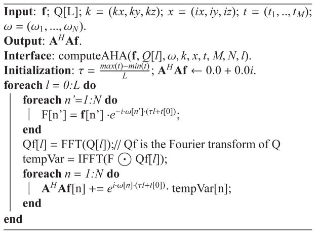
Algorithm 1 shows the pseudo-code for computing A^HAf given the input image f and Q_l. The implementation starts with modulating the input image f with the field inhomogeneity term and computing the Fourier transform Qf [l] of a Q_l matrix. Note that because only the Fourier transform of Q_l is needed for the subsequent calculation, it is recommended to release the storage space allocated to Q[l] after its Fourier transform Qf [l] is calculated. Then, the inverse Fourier transform is taken on the point-wise product between the two vectors F and Qf [l]. Finally, the output vector A^HA is computed in a cumulative fashion. The symbol ⊙ stands for the point-wise product of two vectors, which produces another vector as the output with each element being the product of the associated elements of the two input vectors.

Algorithm 1.

Compute A^HAf using Q_l, Eq. (10).

2.3. Computing Q_l and F^Hy: The gridding approach

The equations for computing F^Hy and Q_l are quite similar. However, Q_l requires considerably more computation time and memory because it is two-fold bigger in size in each dimension. In our previous work, Q_l and F^Hy were computed directly based on their mathematical definitions [7]. In this paper, we utilize the more computationally efficient but less accurate approximation of gridding.

Eq. (11) can be viewed as a Fourier transform of the signal a_l(t_m). As a result, gridding techniques can be used to compute this discrete Fourier transform efficiently. In our gridding code, each data point in our time-segmented interpolator is convolved with a Kaiser-Bessel window [6], then resampled on a Cartesian grid preparatory to an FFT. The Kaiser-Bessel function is used to determine the weight of the contribution of a sample point onto a grid point, based on the distance between the two. A cutoff distance (i.e., kernel width) is imposed on the Kaiser-Bessel kernel beyond which the contribution is considered to be insignificant. After the Fourier transform, a process called deapodization is used to remove the effect of the chosen interpolation kernel from the resulting transform. Our approach toward efficient gridding on GPU will be described in detail in Section 3.

The main motivation for substituting the direct evaluation of Eq. 11 with gridding is significant reduction in computational complexity. As mentioned previously, using gridding only takes MK³ +V³N³ log(V³N³) arithmetical operations, while the direct evaluation takes MN³ operations to compute the same result. For a hypothetical example with 32,768 k-space points and a 256 × 256 × 128 image, the gridding reconstruction reduces computation time by nearly 3 orders of magnitude. Gridding can be further sped up by non-integer oversampling factors V ∈ [1.0,2.0) with acceptable error levels compared to noise in the data [9].

Although we have not experienced stability problems in our application, we note that our implementation stresses speed over numerical accuracy and stability. A less aggressive approach (e.g., using LSQR [27], or brute force, or no time segmentation) might be appropriate in certain situations where the numerical accuracy and stability are bottlenecks.

2.4. Implementation of the conjugate gradient linear solver

The reconstructed image is found by iteratively solving Eq. (7) by using a conjugate gradient linear solver. The solver terminates when the number of iterations exceeds a threshold. During each iteration, the solver performs a large FFT and inverse FFT, several BLAS and sparse BLAS operations (including multiplication of vectors and sparse matrices, as well as addition, scaling, and scalar multiplication of vectors), and several other computations (such as summation reduction, shifting, and sampling). The linear solver uses NVIDIAs CUDA CUFFT Library [28] for the FFT and inverse FFT operations, and implements the other operations as customized code. CUDA’s cufft-Complex structure type is used to represent complex-valued objects.

2.5. Incorporation of a priori information in the image reconstruction

The IMPATIENT package allows the incorporation of a priori information and constraints into image reconstruction. In addition to prior information that can be incorporated using the weighted-least squares regularization penalty of Eq. (6), it’s also possible to use Eq. (6) within the multiplicative half-quadratic optimization framework [29, 30, 31] to solve more general cost functions of the form

$$\widehat{\mathbf{f}}=arg\underset{\mathbf{f}}{min}{\left|\right|\mathbf{A}R\mathbf{f}-\stackrel{\sim }{\mathbf{y}}\left|\right|}_2^2+\mathrm{\Phi }(\mathbf{f}),$$ (12)

where Φ(f) is an appropriate regularization function (e.g., the popular total variation [32] and ℓ₁ norm penalties, or more complicated penalties that are even more tailored to expected image characteristics (e.g. [33, 34]). Specifically, multiplicative half-quadratic approaches solve Eq. (12) for non-quadratic regularization functions by iteratively solving Eq. (6) while updating the diagonal weight matrix W based on the current estimate of f.

The IMPATIENT package provides two alternative ways to implement the regularization function: 1) Using explicit finite difference calculations through template shift-and-subtract operations. 2) Using sparse matrix vector multiplication to evaluate D^HW^HWD operating on a given vector. The first approach is limited to finite-difference based regularization that imposes spatial smoothness on the image, but requires no effort in managing sparse matrices. Although the second approach requires extra effort to optimize sparse matrix storage and related computations on the GPU, it enables a more general form of regularization. The sparse matrices used for regularization penalties are stored in compressed row format [35, 36] and are able to be tailored by the user to the penalty that fits the prior information that they wish to enforce.

2.6. Overall architecture of the IMPATIENT algorithm

Figure 1 shows a summary of the reconstruction architecture of the Toeplitz-based strategy in IMPATIENT. The Toeplitz reconstruction algorithm in IMPATIENT consists of three steps: computing the data structure Q_l, computing the vector F^Hy, and solving the linear system for the image iteratively via a conjugate gradient linear solver. The two selector switches select between direct evaluation (previous implementation) and gridding (current work) for the computation of Q_l and F^Hy.

Figure 1.

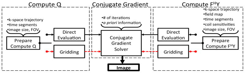
Overview of the entire reconstruction pipeline of the Toeplitz-based strategy in IMPATIENT. The Toeplitz strategy implemented in IMPATIENT provides two ways to compute Q_l and F^Hy. The black solid line is the direct evaluation approach introduced in our previous work [7]. Alternatively, the red dashed line represents the faster gridding alternative proposed in this paper.

3. Gridding on GPU

Although Toeplitz reconstruction was previously implemented on GPUs [7], the use of the direct evaluation approach for calculation of Q_l and F^Hy on GPUs has been impractical for 3D high-resolution data. Despite significant speed-ups over CPU implementations, the direct matrix-vector evaluation approach cannot provide the needed reconstruction speed for such large problems. Alternatively, gridding provides an approximation of these computationally costly operations. Therefore, the remainder of this section describes the gridding algorithms for computing F^Hy and Q_l efficiently on the GPU.

Implementing a gridding algorithm on a GPU can be challenging. As demonstrated in Figure 2, CPU gridding algorithms are traditionally implemented in an input driven approach, where every sample point contributes to all of the grid points within the neighborhood defined by the gridding kernel width, which results in an O(M) algorithm instead of an O(N³M) one, where M is the number of non-Cartesian input sample points and N³ is the number of image locations, which is proportional to the number of Cartesian grid output elements. Mapping the input-driven approach naively onto a GPU’s vector architecture, each k-space point is assigned to a different parallel processing unit. If all the k-space points are processed in parallel, inputs attempting to update the same output element may suffer from data races. This results in multiple processing elements potentially writing to the same output grid point simultaneously, which will lead to incorrect results in the absence of time consuming synchronization. The three input elements highlighted in Figure 2 (left) may suffer from a data race if they attempt to update their shared output simultaneously. However, ensuring this synchronization is costly and can deteriorate the computing performance, especially when several threads try to simultaneously update the same element, since atomic operations causes threads’ updates to be serialized. Several previous methods have been published which implement gridding on the GPU, including [10, 11, 12]. They rely either on atomic operations to handle data races or particular data acquisition trajectory structures to allow for straightforward combination of multiple points gridded to the same location, such as for radial trajectories in [10] or for radial and spiral with a pre-processing distribution plan in [11]. In contrast to these methods, and required for our target application, we develop here a gridding algorithm that handles any non-Cartesian 3D trajectory.

Figure 2.

Parallel implementations of the gridding algorithm on GPU. Left: the output-driven approach is free of write-conflict contention, but has a quadratic computational complexity; Right: Using compact binning as a data pre-processing step allows the output-driven approach to complete in linear time.

The alternative approach to the commonly used input-driven algorithm is an output-driven algorithm, where every output is computed by a single processing thread and all the processing elements share the input elements in a read-only manner. By letting each thread compute exclusively the value of an output grid point, data races are avoided while calculating the contributions from all the neighboring input k-space sample points. By privatizing the output among the threads, multiple output may end up reading the same input elements. Since read accesses do not modify the input elements’ values, no synchronization is needed. However, in arbitrary 3D k-space sampling patterns, the sample point locations cannot simply be inferred nor can neighboring sample points be calculated analytically. Every output element must check each of the M sample points to determine which fall within its cutoff before computing their contribution. The result is an O(MN³) algorithm, despite the amount of useful computation being only O(N³).

The GPU-accelerated gridding algorithm in IMPATIENT is adapted from the work of Obeid et al. [13]. It is an optimized, output-driven algorithm, where every output pixel is computed by a single thread and the input k-space data is shared among all the threads. Input binning is used to ensure that the output-driven gridding algorithm runs in the same O(M) time as the traditional input-driven approach does on the CPU. This is achieved by sorting the k-space points into bins with nonuniform capacity and regular k-space coordinates. Overlapping computations on CPU and GPU is used to further improve the load imbalance caused by varying bin sizes. A bin is a container corresponding to a sub-region of the k-space containing all of the input points that fall within this space. These containers have known characteristics, such as the size of the sub-regions they cover and their element capacity, and this makes them easier to access than individual input elements. Easy access to input elements is enabled by placing them within the bins. Instead of each output element having to traverse the array of all the input elements, it only needs to access the bins that fall within its kernel width to get to the neighboring input elements. Figure 2 (right) depicts the execution of the output-driven approach with binning. Note that some elements that fall within a neighboring bin may not themselves be neighbors of the output element, so it is still necessary to calculate their distance from the output before computing their contribution. In fact binning cannot completely prevent an output from reading input elements that are outside of its kernel width, but it can reduce the number of these occurrences significantly.

3.1. Compact binning based gridding on GPU

One simple way to make all the bins easily accessible is to make them all identical (equal in capacity). This is referred to as regular binning in Figure 3. This bin configuration provides ease of access to the bin, and better control over coalescing and alignment of memory accesses. However, in a non-Cartesian acquisition, the k-space sampling density can vary substantially from region-to-region in k-space, such as in spiral trajectories where the sample density is much higher in the center of the trajectory than it is on the outside. To maintain a uniform size for all the bins, the incurred large memory requirement from padding renders the regular binning infeasible.

Figure 3.

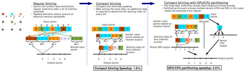
Illustration of regular binning, compact binning and partitioned execution of compact binning based GPU gridding.

In this situation, compact binning is necessary to eliminate the need for padding, see compact binning in Figure 3. The main idea behind compact binning is to allow each bin to have its own bin depth regardless of all the other bins. As a result, the overhead of memory padding is eliminated, and the size of the bin data structure becomes only as large as the number of input elements. The variable bin depth and elimination of padding come at the expense of more complicated access methods to these bins. Since the size of each bin is independent of all the other bins, accessing a bin can no longer be computed as a function of the bin index and the bin capacity. Therefore, additional overhead is incurred in trying to determine the starting offset of each bin. The added overhead stems from the need to pre-compute the starting index of every bin and store it in an array which will then be used as a look-up table for accessing the bins during the gridding.

The compact binning algorithm implemented as part of our GPU-accelerated gridding algorithm consists of four steps: (1) Determine the size of each input bin. (2) Determine the starting index of every bin. (3) Binning the input k-space sample points. (4) Perform the gridding operation by convolving the input points in the bins with the Kaiser-Bessel kernel.

Step 1

The size of each input bin calculated in this step will be used to determine the starting index of each bin. The basic idea is to determine, for each input point, the bin index it belongs to and to count the total number of input elements that are all put in the same bin. Determining the bin sizes can be done either on the CPU sequentially or on the GPU in parallel. In fact, IMPATIENT implements both versions and uses the CUDA NO SM 11 ATOMIC INTRINSICS macro to branch between the two based on the GPU version. The sequential CPU version is necessary for GPUs with compute capability 1.0, in which atomic updates of global memory are not supported. The bin size calculation starts with a zero-initialized integer array of a size equal to the number of bins, and as each k-space point is visited and its bin index determined, the integer corresponding to that bin is incremented by 1. When performed in parallel on GPU, generating the integer array is simply done using atomic updates into the array.

Step 2

The operation that determines the start of each bin is called an exclusive prefix sum [37]. Since each entry in the bin size array (from Step 1) corresponds to the size of a bin, computing the starting offset of a bin corresponds to the sum of the sizes of all the bins that precede it. The prefix sum can be explained as follows. Let p be an index of some element in an array, the exclusive parallel prefix operation computes for each i, except i = 0, the sum of all the elements from index 0 to index i − 1. Our GPU implementation of the parallel prefix sum is a variant of the work by Mark Harris in GPU Gems 3 [38], with a few optimizations applied to achieve more efficient memory usage.

Step 3

Using the starting index of every bin recorded in Step 2, Step 3 places each input element in its correct bin. Similar to Step 1 and 2, this step is also implemented in two ways (namely, both sequentially and in parallel) to accommodate all GPU series. In order to perform binning, another zero-initialized integer array of offsets into each bin is needed to determine the offset within the bin at which to place a given input element. The offset array is important because multiple input points may have the same bin index and we do not want to put them all in the same location in the bin. For each input element, we determine once again the bin it belongs to, place it at the current offset within the bin, then increment the offset. If performed in parallel, binning can be achieved by atomically incrementing the offset counter, and the effects of this atomicity are not too severe, since the only contention is between elements trying to update the same bin, and all other bins can be populated in parallel.

Step 4

In order to perform the actual parallel gridding on GPU, the output grid is first divided into tiles, where each tile is a subset of spatially local output grid points. Each tile is assigned to a thread block where every thread computes exclusively the result of one or more output elements from that subset. The spatial locality of the output in a tile is important to maximize sharing of input data among threads within the block. Algorithm 2 shows the pseudo code for the gridding computation. sharedLocalBin is an array in shared memory that is accessible by all the threads within a block. Each thread is shown to compute only one output element and compute that output’s index based on the 2D blockIdx and 3D threadIdx. Since every thread computes an output element exclusively, the result can be accumulated on-chip in a local register.

Algorithm 2.

Pseudo code for parallel gridding operation on GPU with the compact binning.

00	__shared__ inElem sharedLocalBin[/*max size*/];
01	outputIdx index = computeOutputIndex(blockIdx, threadIdx);
02	outElem myOutElem = initOutElem(index);
03	int zLo = z0 cutoff;
04	int zHi = z0 + blockDim.z + cutoff;
05	// compute yLo, yHi, xLo, xHi similarly
06	for z = [zLo:zHi]{
07	for y = [yLo:yHi]{
08	for x = [xLo:xHi]{
09	int start = binOffsetArray[z][y][x];
10	int end = binOffsetArray[z][y][x+1];
11	if(threadIdx < end-start){
12	sharedLocalBin[threadIdx] = globalBinArray[start+threadIdx];
13	}
14	__syncthreads();
15	for i=[0:end-start]{
16	if(|sharedLocalBin[i].coords myOutElem.coords| < kernel-width){
17	/*compute the contribution of this input onto the output*/
18	} } } } }
19	globalOutputGrid[index] = myOutElem;

Every output element is computed by a single thread exclusively, and that thread can compute the value of that element locally (line 2). Every block iterates over all the bins that its output tile intersects: zLo to zHi, yLo and yHi, and xLo to xHi are the 3D bounds of the region intersected by a given tile. for each bin that is visited, all of its elements are loaded cooperatively into shared memory by all the threads in the block. Note that a bin is visited if at least one of the outputs within the block’s tile intersects that bin; however, that bin may fall outside the kernel width of other outputs in the tile. That is why it is still necessary to check whether a given input point is within the kernel width of the output point before computing its contribution to that output (Line 15). Once all the bins and all the elements within them have been inspected, and their contributions added, each thread writes its privately computed output to the global array that is the final result. binOffsetArray in line 9 and 10 stores the starting offsets of the bins generated in Step 2 when performing the input binning and is used to determine how many elements are in a given bin.

Two comments about the efficient use of global and shared memory are important for our implementation. The first important implementation detail is that, instead of accessing each bin separately as shown in Algorithm 2, an entire range of contiguous bins is accessed simultaneously in the actual code. More specifically, for any given z and y bin coordinates, bins xL through xH, which occupy consecutive memory locations, can all be loaded simultaneously since compact bins do not contain any padding elements; all the elements between the start of xL and xH are in fact useful to the computation and all need to be loaded into on chip memory. For that reason, rather than simply reading the start of each bin and the one following it to determine the range of a single bin in x, we can read the start and end indices of the entire range in x once, and load all the elements within that range into on chip memory. The benefits of this optimization are three-fold. First, the number of accesses to the bin offset array is reduced from two accesses per bin to two accesses amortized over the number of bins within the range. Second, the access into the bins is more efficient as memory bursts are better utilized by not breaking bins’ bounds. Finally, by accessing entire ranges rather than individual bins, the loop for the x dimension is removed, thereby reducing the overall number of loops within the kernel.

Another comment concerns the optimal data layout in global memory. One of the potential drawbacks of compact binning is the resulting misalignment of bins in memory. To fix the misalignment, the actual implementation lays out the input elements in the form of arrays of float vector types (float2) since the effect of misalignment on float2 arrays is less severe than on single float arrays. This approach involves a reorganization of the bin data structures from array of structures to structure of arrays. Sung et al. discuss the benefits of this transformation in their work [39]; however, unlike the strided access pattern they discuss, in our case, all the elements within the structures are of the float type, we can have every thread load a single float element from within the structure to shared memory, thus maintaining a coalesced access since the stride of the access is one. Since the accesses into the array of structures are already coalesced, laying out the data in a structure of array format is not expected to significantly impact the performance. However, if we laid out the data in a structure of short vector arrays, we would expect to see better performance for misaligned accesses.

Finally, to improve load balance, the gridding task is partitioned evenly between the GPU and CPU. A bin depth is determined that achieves the optimal balance between CPU and GPU execution, and all of the elements that exceed this bin depth are offloaded to the CPU when performing binning. Since kernel execution on the GPU is asynchronous to the CPU, the optimal bin depth is defined as that which results in equal execution time on the GPU and CPU. Figure 3 compares regular binning, compact binning and the execution model for the partitioned compact bins.

4. Experimental results and discussions

This work uses the NVIDIA Tesla M2070 GPU as the hardware target for its advanced MRI reconstruction study. The Tesla M2070 is an example of a Fermi based graphics card, which consists of 448 CUDA cores, with groups of 32 CUDA cores being organized into 14 Stream Multiprocessors (SM). Running at 1.15 GHz, the Tesla M2050 GPU coprocessor is rated at 1288 GFLOPS of peak theoretical performance (single precision).

4.1. Diffusion Weighted Imaging as an Enabled Application

High resolution 3D diffusion weighted imaging (DWI) is a technique that requires significant computational power in order to reconstruct images. In addition to large image sizes, high resolution images also typically are acquired using multiple receiver coils, requiring parallel imaging, and using long readouts, making field inhomogeneity correction desirable. Additionally, multi-shot diffusion imaging is subject to errors from subject motion during diffusion encoding. These motion induced phase errors result in random shifts of the k-space trajectories and random offset phase in the data [40, 41]. Correcting for these errors results in k-space trajectories that are shifted for each shot and are unique to each acquisition. A stack-of-spirals 3D acquisition would normally allow for separate FFT in the slice direction prior to 2D processing of each slice. However, with the motion-induced phase errors in diffusion imaging, each shot of the stack of spirals acquisition is randomly shifted resulting in a truly 3D trajectory, requiring a 3D reconstruction. The motion-induced phase errors are estimated by collecting navigator data associated with each line of k-space through an additional echo in the acquisition, see [41] for details on the sequence, navigation, and estimation of k-space shifts from the navigator.

Normally Q_l can be pre-computed because it only depends on k-space trajectory and image size. However with multi-shot diffusion imaging, the k-space trajectory is not known prior to the data acquisition. This causes a need for a new Q_l to be computed for each acquisition of a 3D data set. The performance of IMPATIENT MRI was tested on five 3D diffusion imaging datasets with imaging matrix sizes ranging from 32x32x4 to 256x256x32, for benchmarking purposes. The 3D datasets are multi-shot stack of constant density spirals with matrix size in the x and y directions increased with an accompanying increase in the number of spiral interleaves and the z dimension increased by increasing the number of phase encoding steps. Although the data would normally be amenable to gridding in-plane and a separate FFT across the slice direction, due to motion-induced phase errors in diffusion, the resulting k-space trajectories are truly 3D and change for each data set. The ability to efficiently calculate Q, makes IMPATIENT an ideal platform for reconstructing images in cases where many k-space trajectories are possible, such as in DWI.

Additional parallelization of the MRI image reconstruction problem is possible for data sets, such as DWI, that acquire multiple volumes. DWI data sets acquire multiple image volumes and multiple diffusion directions, all of which must be reconstructed to visualize the underlying physical process of interest. Access to computational nodes with multiple GPUs can provide trivial acceleration over the multiple volumes to be reconstructed.

4.2. Performance measurements and results

To evaluate the performance of our GPU gridding implementation, we isolate the gridding GPU kernels into a standalone application and compare execution time with the CPU code implementing the same gridding algorithm. Performance measurements on a Tesla M2070 GPU show that the proposed output-driven gridding GPU implementation achieves a performance of 4.3 GFLOPS in single floating-point calculation for an image size of 240x240x32. The achieved speedup is 26.3-fold compared to the same algorithm implemented on a single CPU core. All kernels, including the two binning steps, prefix sum and the actual gridding operations, are considered in the measurement of GFLOPS rate. The amount of memory on Tesla M2070 (6 Gbytes) limits the grid size to no more than 256x256x128 in single precision on the GPU. In order to measure the performance in GFLOPS on a GPU, given a fixed data set, the number of floating point operations of the CPU code is counted using the performance counters provided by the Performance API (PAPI) [42]. Then, the GPU performance (in terms of GFLOPS) is evaluated using the obtained counts and the GPU computation time. The CPU performance of the original CPU code written in C++, implementing the identical gridding algorithm, is measured on a 3.3 GHz Xeon E5520 CPU and calculations are also done in single precision.

The proposed GPU gridding algorithm was implemented as an integral part of the Toeplitz reconstruction strategy of IMPATIENT. Our GPU gridding code provides a fast approximation to the direct evaluation of Q_l and F^Hy. The performance of the Toeplitz strategy equipped with GPU gridding was compared with that of the original Toeplitz implementation using direct evaluation [7]. All reconstructions were performed on the same workstation. The speed benefit of the new gridding-accelerated Toeplitz strategy is substantial as demonstrated by typical image sizes in Figure 4 and 5. All reconstructions execute 10 conjugate gradient iterations and use 8 time segments. To emphasize speed over accuracy, a gridding oversampling factor of 1.4 is chosen for both Q_l and F^Hy. The gridding kernel width is hard-coded to 4 (measured in Nyquist k-space sampling distances) and the rest of the gridding parameters are determined based on the results in [9]. The execution timings are broken down into three steps. The baseline algorithm for comparison is the basic Toeplitz strategy, which evaluates Q_l and F^Hy using direct evaluation of the matrix-vector products [7]. Using a Tesla M2070, five 3D DWI data sets were tested: 256x256x32, 240x240x32, 128x128x16, 64x64x16 and 32x32x4. All data was acquired with on a Siemens 3 T MRI scanner with 4 receiver coils, using a custom-designed multi-shot 3D stack-of-spirals DWI sequence, with 4-shots covering the in-plane encoding and separate shots for each slice encoding. The sequence includes a second echo for the navigator acquisition which is a sigle-shot, low-resolution stack-of-spirals to allow for estimation of phase errors associated with each shot of the high-resolution acquisition. The images were reconstructed with a SENSE reconstruction, although full data sampling was acquired [5]. Due to random shifts of the k-space trajectories, some undersampling will occur at random and the SENSE reconstruction provides a robust reconstruction despite these random trajectory shifts. All data was acquired on healthy volunteers in accordance with the local Institutional Review Board. All calculations are done in single precision mode.

Figure 4.

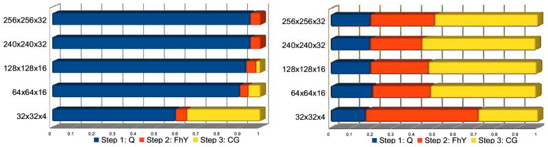
Percentage of computation time spent in each step. Left: The baseline Toeplitz strategy with the direct evaluations of Q_l and F^Hy; Right: The fast Toeplitz strategy with Q_l and F^Hy computed via the GPU-accelerated gridding. The total execution times are normalized between 0 and 1 to emphasize the relative time of each step. For comparison, Step 3 is identical for both methods. The performance benefits from gridding are clearly demonstrated by the reduction of the fraction of the time spent in Steps 1 and 2.

Figure 5.

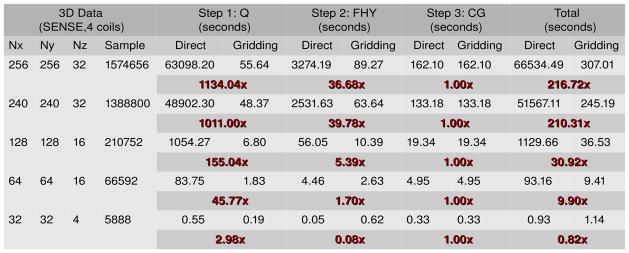
The execution time and the computational speedup between the two versions of the Toeplitz reconstruction strategy on one Tesla M2070 GPU. In step 1, a reduction in execution time of 17.5 hours (63098.20 s to 55.64 s, about 1134x speedup) was obtained for the image size of 256x256x32 with 1574656 input samples per coil. Note that Step 3 takes the same amount of time across the two versions as they use the same conjugate gradient solver.

Cylinder charts in Figure 4 show the ratio of computing time spent in each of the three steps during reconstruction of the five data sets. The length of the cylinder represents the normalized total execution time. In the baseline Toeplitz strategy with the direct evaluation (Figure 4, Left), the time spent on the CG step (Step 3) is negligible (less than 0.5% for larger data sizes) compared to the combined time spent on Steps 1 and 2. Furthermore, the corresponding execution pipeline is highly unbalanced as the first two steps dominates the pipeline. With the performance contributed by gridding, the gridding-accelerated Toeplitz strategy (Figure 4, Right) becomes much more balanced. The proportional times spent on Steps 1 and 2 become closer to that spent on Step 3, making the total runtime almost evenly distributed among the pipeline. In summary, we observed consistent decreases in computation time by using gridding, with the maximum speedups of more than 1134x in Step 1 and 39x in Step 2. An interesting exception is 32x32x4, where in Step 2 we see a slowdown instead of a speedup. This is likely due to the eight time segments for the time-segmented gridding approach requiring eight sets of weighting, convolution, and FFT. The FFT’s require synchronization prior to computation, incurring some time penalty on the GPU. However, direct calculation of the Toeplitz formulation fits well with the ideal GPU problem, small amount of data per kernel and large amounts of computation without a required synchronization. The small sized problem results in a very quick direct evaluation on the GPU, with no time segmentation and only final synchronization needed. This shows that the direct evaluation Toeplitz is faster on small data sizes than the gridding-accelerated Toeplitz. It is interesting to note that for the CPU, there is less penalty in the required synchronization for the FFT and there is no capability for massively parallel calculations in the Toeplitz formulation. So this tradeoff of problem size and computation time is expected to be different for GPU than for CPU.

As a comparison of our computational time performance with a previously implemented gridding reconstruction, we can examine just the component F^Hy, which is equivalent to a time-segmented gridding reconstruction across all coils. In our results, we see that for a 256x256x32 reconstruction, the time for gridding was 89.27 s on the GPU. If we divide this number by the 32 slices, the 4 coils, and the 8 time segments, we get a value of 0.09 s per 256x256 gridding. However, this gridding time for our technique includes all of the operations of binning, coil sensitivity weighting, multiplication of phase maps for the field inhomogeneity correction, and time interpolation. As a comparison, in [11], for a 2D spiral with a matrix size of 256x256, they obtained 0.02 s for gridding with no coil sensitivities or field inhomogeneity. Additionally, in [11], they used a precomputed kernel to determine how to assign incoming data points to particular GPU kernels to handle the overlapping contributions from data. In our method, the time to compute the plan is included in the gridding operation. If gridding of fixed trajectories is desired, other gridding implementations may be more efficient where they can leverage pre-computed data structures. However, for a general gridding technique, our gridding algorithm performs at a similar rate without the need for precomputed plans.

Figure 6a and 6b shows two reconstructed brain images from a high resolution diffusion imaging scan reconstructed with the IMPATIENT reconstruction utility. It gives the reconstruction results for the gridding-accelerated Toeplitz strategy using a 240x240x32 matrix size and a full SENSE parallel imaging reconstruction with and without field inhomogeneity correction. Notice that the field inhomogeneity correction reduces the blurring induced by magnetic field inhomogeneities.

Figure 6.

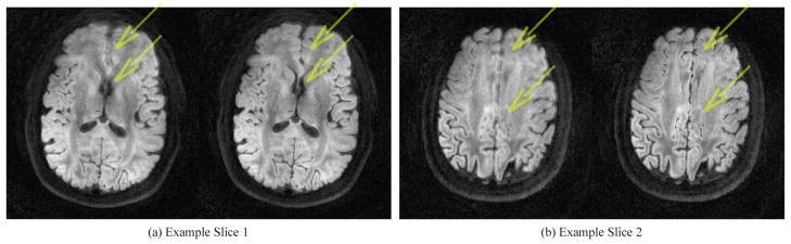
Two pairs of reconstructed images to demonstrate the effect of the field inhomogeneity correction for 3D DWI on GPU. Left: SENSE reconstruction without field inhomogeneity correction; Right: SENSE reconstruction with field inhomogeneity correction. The blurring artifacts, which is most noticeable around the area pointed to by the arrows, have been reduced considerably with field inhomogeneity correction.

5. Conclusion

This paper describes the gridding-accelerated IMPATIENT MRI reconstruction toolkit which can achieve clinically-feasible 3D, non-Cartesian, field-inhomogeneity corrected, regularized, iterative image reconstruction from parallel acquisition arrays in MRI. We have shown that, through the use of gridding on the GPU, we are able to diminish the computational barrier associated with non-Cartesian, arbitrary trajectory MRI reconstructions and facilitate incorporation of advanced image acquisition and reconstruction techniques in the clinic. Our toolkit has demonstrated the feasibility of utilizing GPU compute power to inject computational intensive algorithms into the advanced MRI reconstruction workflow while maintaining clinically-relevant reconstruction times on the order of minutes. As a proof of concept, we demonstrated a 3D DWI application enabled by the IMPATIENT MRI package. The same application, would otherwise take too long for both clinical and research imaging practitioners, requiring up to 15 hours with a previous GPU-accelerated software platform compared to 5 minutes with the current IMPATIENT MRI software. The IMPATIENT MRI software package is available for download at our web site: http://impact.crhc.illinois.edu/mri.php.

• GPU-accelerated software toolkit for arbitrary 3D non-Cartesian trajectories in MRI.

• Incorporate parallel imaging, magnetic field correction, and a priori information.

• Enables clinically-feasible image reconstruction times for advanced acquisitions.

• Achieved 200 times speed-up over previous GPU image reconstruction algorithm.

Biographies

Jiading Gai is currently a postdoc researcher in Bioengineering and the Beckman Institute for Advanced Science and Technology at the University of Illinois at Urbana-Champaign. Dr. Gai received his B.S. degree in automation and M.E. degree in pattern recognition from Tsinghua University in 2001 and 2004, and M.S. degree in applied mathematics and Ph.D. degree in computer vision from University of Notre Dame in 2007 and 2010. His research interests focus on developing GPU scientific computing applications..

Nady Obeid completed a Masters in Computer Engineering under Prof. Wen-Mei Hwu in Dec 2010. His research led to the application of a sparse data structure optimization to the gridding step in MRI reconstruction. He is currently a software engineer at KLA-Tencor focusing on high-performance computing using various architectures and programming languages.

Joseph L. Holtrop is a Ph.D. candidate in Bioengineering at the University of Illinois at Urbana-Champaign. He received his B.S. degree in Electrical and Computer Engineering from Calvin College in 2009. He received his M.S. degree in Bioengineering from University of Illinois in 2012. His research interests include data acquisition and image reconstruction, with a focus on diffusion weighted imaging and its applications.

X.-L. Wu is a Ph.D. candidate in Electrical and Computer Engineering and a graduate research assistant in the IMPACT research group at the University of Illinois at Urbana-Champaign. He received his B.S. and M.S. degrees in Computer Science and Engineering in 1999 and 2001, respectively all in Yuan-Ze University, Taiwan. His research interests involve compiler design for parallelism, application acceleration, and debugging and performance tuning for many-core parallelism. His current researches include the acceleration of magnetic resonance image reconstruction and the development of DNA sequence assembly algorithms.

Fan Lam is a Ph.D. candidate in Electrical and Computer Engineering at the University of Illinois at Urbana-Champaign. He received his B.S. degree in Biomedical Engineering from Tsinghua University, China, in 2008. He received his M.S. degree in Electrical and Computer Engineering from University of Illinois, in 2011. His research interests include data acquisition, image reconstruction, denoising and parameter estimation for magnetic resonance imaging, with focus on high resolution brain imaging. Fan is also a recipient of Computational Science and Engineering Fellowship and Beckman Fellowship at University of Illinois.

Maojing Fu is a Ph.D. candidate in electrical and computer engineering at the University of Illinois at Urbana-Champaign. He received the B. S. degree in electrical science and engineering from Nanjing University in China in 2010. He received the M. S. degree in electrical and computer engineering from the University of Illinois at Urbana-Champaign in 2012. He is interested in data acquisition, image reconstruction and physiological modeling methods for dynamic magnetic resonance imaging.

J. P. Haldar received the Ph.D. degree in Electrical and Computer Imaging from the University of Illinois at Urbana-Champaign in 2011. He is currently an Assistant Professor in the Ming Hsieh Department of Electrical Engineering at the University of Southern California. His research interests include multidimensional signal processing, parameter estimation, experiment design, and inverse problems, with a primary focus on the development of new data acquisition and signal processing methods for improved and accelerated magnetic resonance imaging.

W.-m.W. Hwu is a Professor and holds the Walter J. (“Jerry”) Sanders III-Advanced Micro Devices Endowed Chair in Electrical and Computer Engineering of the University of Illinois at Urbana-Champaign. His research interests are in the area of architecture, implementation, and compilation for parallel computer systems. He directs the IMPACT research group (www.crhc.uiuc.edu/Impact). For his contributions, he received the ACM SigArch Maurice Wilkes Award, the ACM Grace Murray Hopper Award, and the ISCA Most Influential Paper Award. He is a fellow of IEEE and ACM. Hwu received his Ph.D. degree in Computer Science from the University of California, Berkeley in 1987..

Z.-P. Liang received his Ph.D. degree in Biomedical Engineering from Case Western Reserve University in 1989. He is currently Professor of Electrical and Computer Engineering at the University of Illinois at Urbana-Champaign. He is also affiliated with the Beckman Institute for Advanced Science and Technology, the Computational Biophysics Program, and the Department of Bioengineering. Dr. Liang’s research interests include magnetic resonance imaging, superresolution image reconstruction using a priori constraints, statistical and learning-based methods for biomedical image analysis, and their application to functional brain mapping, cancer imaging, and cardiac imaging.

B.P. Sutton is currently an Associate Professor in Bioengineering and the Beckman Institute for Advanced Science and Technology at the University of Illinois at Urbana- Champaign. Dr. Sutton received M.S. degrees in Biomedical and Electrical Engineering (2001) and a Ph.D. in Biomedical Engineering from the University of Michigan in 2003. Dr. Sutton’s research focuses on development of novel acquisition techniques in structural and functional brain imaging.

References

- 1.Pruessmann KP, Weiger M, Scheidegger MB, Boesiger P. SENSE: Sensitivity encoding for fast MRI. Magn Reson Med. 1999;42:952–962. [PubMed] [Google Scholar]
- 2.Sekihara K, Kuroda M, Kohno H. Image restoration from non-uniform magnetic field influence for direct fourier nmr imaging. Phys Med Biol. 1982;29:15–24. doi: 10.1088/0031-9155/29/1/002. [DOI] [PubMed] [Google Scholar]
- 3.Sutton BP, Noll DC, Fessler JA. Fast, iterative image reconstruction for MRI in the presence of field inhomogeneities. IEEE Trans Med Imaging. 2003;22:178–188. doi: 10.1109/tmi.2002.808360. [DOI] [PubMed] [Google Scholar]
- 4.Fessler J. Model-based image reconstruction for MRI. IEEE Signal Processing Magazine. 2010;27:81–89. doi: 10.1109/MSP.2010.936726. [DOI] [PMC free article] [PubMed] [Google Scholar]
- 5.Pruessmann KP, Weiger M, Bornert P, Boesiger P. Advances in sensitivity encoding with arbitrary k-space trajectories. Magn Reson Med. 2001;46:638–51. doi: 10.1002/mrm.1241. [DOI] [PubMed] [Google Scholar]
- 6.Jackson JI, Meyer CH, Nishimura DG, Macovski A. Selection of a convolution function for fourier inversion using gridding. IEEE Trans Med Imaging. 1991;10:473–478. doi: 10.1109/42.97598. [DOI] [PubMed] [Google Scholar]
- 7.Stone SS, Haldar JP, Tsao SC, Hwu W-MW, Sutton BP, Liang Z-P. Accelerating advanced MRI reconstructions on GPUs. J Parallel Distrib Comput. 2008:1307–1318. doi: 10.1016/j.jpdc.2008.05.013. [DOI] [PMC free article] [PubMed] [Google Scholar]
- 8.Zhuo Y, Wu X-L, Haldar JP, Marin T, Hwu W-M, Liang Z-P, Sutton BP. Using GPUs to accelerate advanced MRI reconstruction with field inhomogeneity compensation. In: Hwu W-M, editor. GPU Computing Gems. Morgan Kaufmann Publishers; 2010. [Google Scholar]
- 9.Beatty PJ, Nishimura DG, Pauly JM. Rapid gridding reconstruction with a minimal oversampling ratio. IEEE Trans Med Imaging. 2005;24:799–808. doi: 10.1109/TMI.2005.848376. [DOI] [PubMed] [Google Scholar]
- 10.Schiwietz T, chiun Chang T, Speier P, Westermann R. Mr image reconstruction using the gpu. Proc. SPIE; p. 6142. [Google Scholar]
- 11.Sorensen TS, Schaeffter T, Noe KO, Hansen MS. Accelerating the nonequispaced fast fourier transform on commodity graphics hardware. IEEE Trans Med Imaging. 2008;27:538–547. doi: 10.1109/TMI.2007.909834. [DOI] [PubMed] [Google Scholar]
- 12.Gregerson A. Technical Report. NVIDIA Tech; 2008. Implementing fast MRI gridding on GPUs via CUDA. Report on Medical Imaging using CUDA. [Google Scholar]
- 13.Obeid NM, Atkinson IC, Thulborn KR, Hwu W-MW. GPU-accelerated gridding for rapid reconstruction of non-cartesian MRI. Proc Intl Soc. for Magn Reson Med (ISMRM); 2011. p. 2547. [Google Scholar]
- 14.Roujol S, de Senneville BD, Vahala E, Sorensen TS, Moonen C, Ries M. Online real-time reconstruction of adaptive TSENSE with commodity CPU/GPU hardware. Magn Reson Med. 2009;62:1658–1664. doi: 10.1002/mrm.22112. [DOI] [PubMed] [Google Scholar]
- 15.Sorensen TS, Atkinson D, Schaeffter T, Hansen MS. Real-time reconstruction of sensitivity encoded radial magnetic resonance imaging using a graphics processing unit. IEEE Trans Med Imaging. 2009;28:1974–1985. doi: 10.1109/TMI.2009.2027118. [DOI] [PubMed] [Google Scholar]
- 16.Nam S, Akcakaya M, Basha T, Stehning C, Manning WJ, Tarokh V, Nezafat R. Compressed sensing reconstruction for whole-heart imaging with 3d radial trajectories: A graphics processing unit implementation. Magn Reson Med. 2012 doi: 10.1002/mrm.24234. In press. [DOI] [PMC free article] [PubMed] [Google Scholar]
- 17.Uecker M, Hohage T, Block KT, Frahm J. Image reconstruction by regularized nonlinear inversion – Joint estimation of coil sensitivities and image content. Magn Reson Med. 2008;60:674–682. doi: 10.1002/mrm.21691. [DOI] [PubMed] [Google Scholar]
- 18.Knoll F, Unger M, Diwoky C, Clason C, Pock T, Stollberger R. Fast reduction of undersampling artifacts in radial MR angiography with 3D total variation on graphics hardware. MAGMA. 2010;23:103–114. doi: 10.1007/s10334-010-0207-x. [DOI] [PMC free article] [PubMed] [Google Scholar]
- 19.Knoll F, Bredies K, Pock T, Stollberger R. Second order total generalized variation (TGV) for MRI. Magn Reson Med. 2010;65:480–491. doi: 10.1002/mrm.22595. [DOI] [PMC free article] [PubMed] [Google Scholar]
- 20.Murphy M, Alley M, Demmel J, Keutzer K, Vasanawala S, Lustig M. Fast ℓ1-SPIRiT compressed sensing parallel imaging MRI: scalable parallel implementation and clinically feasible runtime. IEEE Tran Med Imaging. 2012;31:1250–62. doi: 10.1109/TMI.2012.2188039. [DOI] [PMC free article] [PubMed] [Google Scholar]
- 21.Wu X-L, Gai J, Lam F, Fu M, Haldar JP, Zhuo Y, Liang Z-P, Hwu W-MW, Sutton BP. IMPATIENT MRI: Illinois massively parallel acceleration toolkit for image reconstruction with enhanced throughput in MRI. Proc of IEEE Intl Symp Biomed Imaging; 2011. pp. 69–72. [Google Scholar]
- 22.Wajer FTAW, Pruessmann KP. Major speedup of reconstruction for sensitivity encoding with arbitrary trajectories. Proc Intl Soc. for Magn Reson Med (ISMRM); 2001. p. 767. [Google Scholar]
- 23.Fessler JA, Lee S, Olafsson VT, Shi HR, Noll DC. Toeplitz-based iterative image reconstruction for MRI with correction for magnetic field inhomogeneity. IEEE Trans Signal Process. 2005;53:3393–3402. [Google Scholar]
- 24.Haldar J, Hernando D, Song S-K, Liang Z-P. Anatomically constrained reconstruction from noisy data. Magn Reson Med. 2008;59:810–818. doi: 10.1002/mrm.21536. [DOI] [PubMed] [Google Scholar]
- 25.Shewchuk JR. Technical Report. Carnegie Mellon University; Pittsburgh, PA, USA: 1994. An Introduction to the Conjugate Gradient Method Without the Agonizing Pain. [Google Scholar]
- 26.Noll DC, Meyer CH, Pauly JM, Nishimura DG, Macovksi A. A homogeneity correction method for magnetic resonance imaging with time-varying gradients. IEEE Trans Med Imaging. 1991;10:629–637. doi: 10.1109/42.108599. [DOI] [PubMed] [Google Scholar]
- 27.Paige CC, Suanders MA. Lsqr: An algorithm for sparse linear equations and sparse least squares. ACM Transactions on Mathematical Software. 1982;8:43–71. [Google Scholar]
- 28.NVIDIA Corporation. CUDA CUFFT Library. 2011. Version 4.0. [Google Scholar]
- 29.Nikolova M, Ng MK. Analysis of half-quadratic minimization methods for signal and image recovery. SIAM J Sci Comput. 2005;27:937–966. [Google Scholar]
- 30.Delaney AH, Bresler Y. Globally convergent edge-preserving regularized reconstruction: an application to limited-angle tomography. IEEE Trans Image Process. 1998;7:204–221. doi: 10.1109/83.660997. [DOI] [PubMed] [Google Scholar]
- 31.Charbonnier P, Blanc-Feraud L, Aubert G, Barlaud M. Deterministic edge-preserving regularization in computed imaging. IEEE Trans Image Process. 1997;6:298–310. doi: 10.1109/83.551699. [DOI] [PubMed] [Google Scholar]
- 32.Rudin LI, Osher S, Fatemi E. Nonlinear total variation based noise removal algorithms. Physica D. 1992;60:259–268. [Google Scholar]
- 33.Black MJ, Rangarajan A. On the unification of line processes, outlier rejection, and robust statistics with applications in early vision. Int J Comput Vis. 1996;19:57–91. [Google Scholar]
- 34.Haldar JP, Wedeen VJ, Nezamzadeh M, Dai G, Weiner MW, Schuff N, Liang ZP. Improved diffusion imaging through snr-enhancing joint reconstruction. Magn Reson Med. 2012 doi: 10.1002/mrm.24229. In press. [DOI] [PMC free article] [PubMed] [Google Scholar]
- 35.Dongarra J. Compressed Row Storage (CRS) 2000 http://netlib.org/utk/papers/templates/node91.html.
- 36.Bell N, Garland M. NVIDIA Technical Report NVR-2008-004. NVIDIA Corporation; 2008. Efficient Sparse Matrix-Vector Multiplication on CUDA. [Google Scholar]
- 37.Blelloch GE. Scans as primitive parallel operations. IEEE Trans on Computers. 1989;38:1526–1538. [Google Scholar]
- 38.Harris M, Sengupta S, Owens JD. Parallel prefix sum (scan) with CUDA. In: Nguyen H, editor. GPU Gems 3. Addison Wesley; 2007. pp. 851–876. [Google Scholar]
- 39.Sung I-J, Stratton JA, Hwu W-MW. Data layout transformation exploiting memory-level parallelism in structured grid many-core applications. Proceedings of the 19th international conference on Parallel architectures and compilation techniques, PACT ‘10; ACM, New York, NY, USA. 2010. pp. 513–522. [Google Scholar]
- 40.Anderson AW, Gore JC. Analysis and correction of motion artifacts in diffusion weighted imaging. Magn Reson Med. 1994;32:379–387. doi: 10.1002/mrm.1910320313. [DOI] [PubMed] [Google Scholar]
- 41.Van AT, Hernando D, Sutton BP. Motion-induced phase error estimation and correction in 3D diffusion tensor imaging. IEEE Trans Med Imaging. 2011:1933–1940. doi: 10.1109/TMI.2011.2158654. [DOI] [PubMed] [Google Scholar]
- 42.Browne S, Dongarra J, Garner N, London K, Mucci P. A portable programming interface for performance evaluation on modern processors. Int J High Perform C. 2000;14:189–204. [Google Scholar]