Estimation Using All Available Covariate Information Versus a Fixed Look-back Window for Dichotomous Covariates

Abstract

Purpose

When using claims data, dichotomous covariates (C) are often assumed to be absent unless a claim for the condition is observed. When available historical data differs among subjects, investigators must chose between using all available historical data versus data from a fixed window to assess C. Our purpose was to compare estimation under these two approaches.

Methods

We simulated cohorts of 20000 subjects with dichotomous variables representing exposure (E), outcome (D) and a single time-invariant C, as well as varying availability of historical data. C was operationally defined under each paradigm and used to estimate the adjusted risk ratio of E on D via Mantel-Haenszel methods.

Results

In the base case scenario, less bias and lower MSE were observed using all available information compared with a fixed window; differences were magnified at higher modeled confounder strength. Upon introduction of an unmeasured covariate (F), the all-available approach remained less biased in most circumstances and better approximated estimation that was adjusted for the actual (modeled) value of the confounder in all instances.

Conclusions

In most instances considered, operationally defining time-invariant dichotomous C based on all available historical data, rather than on data observed over a commonly shared fixed historical window, results in less biased estimates.

The validity of epidemiologic findings depends on the completeness and accuracy with which covariates are measured and taken into account. For some variables such as comorbid conditions or concurrent therapies, it is often not possible to distinguish between missing data and absence of the condition. Operationally, missing information for such variables is usually assumed to indicate that the condition is not present.¹ In cohort studies conducted within healthcare utilization databases, the sensitivity with which such variables are detected depends in large part on the duration of time over which each subject had been observed before follow-up began.² Because subjects will vary in terms of the duration of available baseline information, the investigator is faced with a choice: 1) utilize covariate information based on all available baseline data for each subject, 2) utilize covariate information based on a fixed baseline window of time that is shared by all subjects (often chosen as 6 months or 1 year). We term these options the “all-available” and “fixed window” approaches.

It can be assumed that under the all-available paradigm, confounders will be identified with equal or greater sensitivity than under a fixed window approach, which should serve to reduce residual confounding.^3-4 On the other hand, the duration of available baseline data may be associated with subject covariates, subsequent exposure and outcome (each either directly or mediated through other unmeasured confounders), so that the all-available approach could introduce bias through differential confounder ascertainment.

Consider the following motivating example. Investigators are interested in estimating the comparative effectiveness of new use of anti-platelet agent A versus a standard anti-platelet agent B on 30-day stroke risk following a transient ischemic attack among Medicaid beneficiaries in secondary claims data. Diabetes is an important potential confounder. The source cohort comprises patients who have a claim involving a diagnosis code for transient ischemic attack, and who subsequently filled a prescription for anti-platelet medication A or B (index fill). Potential subjects are excluded if they demonstrate claims for anti-platelet agents before the index fill, or if they do not have 6 months of available data before the index fill over which to document no prior exposure. Some patients meeting entry criteria may have the minimum requisite 6 months of baseline data, whereas others may have many years of baseline data. The duration of available data likely relates to observable characteristics (eg, socioeconomic status, disability) as well as unobservable ones (eg, frailty) that themselves are associated with diabetic status, choice of anti-platelet agent and risk of subsequent stroke. To define diabetes, the investigator must determine whether to identify claims suggesting diabetes using all available data for each patient, or to restrict to data from the collectively shared 6-month baseline period. The latter approach results in uniform observation periods for study participants, but that comes at the cost of ignoring some data available for some patients.

We sought to explore the tradeoffs inherent in this choice through a simulation study that compared bias reduction under these two approaches, and to determine the conditions under which one approach may be preferable to the other. Specifically, we considered the following circumstance: 1) the effect of interest was that of a dichotomous exposure on a dichotomous outcome; 2) the observed exposure—outcome association was confounded by a single observed dichotomous covariate; 3) all study subjects included in the analysis had available data for at least the 6-month period preceding exposure, and variable amounts of lead-up time before that period. We then compared the two approaches in the presence of an additional unmeasured covariate that was associated with exposure, outcome, duration of historical follow up and frequency of medical contact. Of note, we have considered confounding based on a chronic disease (or analogous) conception; results do not pertain to covariates that confound on a temporary or transient basis (eg, acute conditions).

MATERIALS AND METHODS

Base case simulation

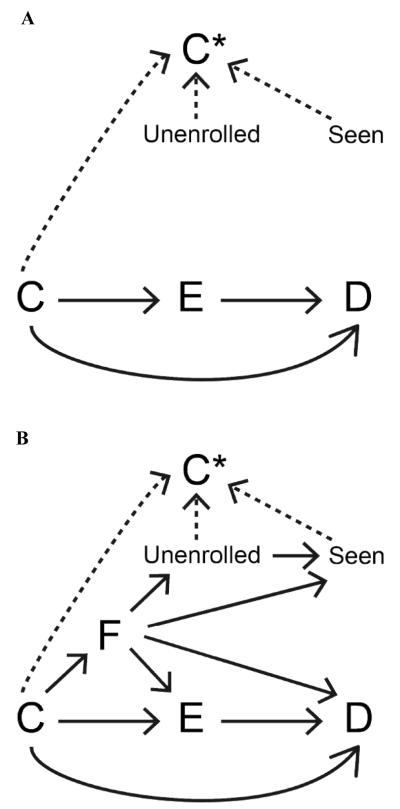
Figure 1a shows the directed acyclic graph used to generate data in the base case. In each replicate we simulated a cohort of 20,000 subjects with three dichotomous variables representing exposure (E), outcome (D) and a single time-invariant confounder (C) based on Bernoulli distributions. Values of C were simulated based on the marginal probability (C=1, termed pc). E was simulated based on the probabilistic model:

$$\mathrm{Pr}(\mathrm{E}=1\mid \mathrm{C}=\mathrm{c})=\mathit{pe}0\ast \mathrm{X}(1+\mathit{rrec}\ast \mathrm{C})$$

where pe0 is the probability of being exposed if C=0, and rrec is the risk ratio of C on E. D was simulated based on the probabilistic model:

$$\mathrm{Pr}(\mathrm{D}=1\mid \mathrm{E}=\mathrm{e},\mathrm{C}=\mathrm{c})=\mathit{pd}0\ast \left[\right(1-\mathrm{E})\ast (1-\mathrm{C})+\mathrm{E}\ast (1-\mathrm{C})\ast \mathit{rrde}+(1-\mathrm{E})\ast \mathrm{C}\ast \mathit{rrdc}+\mathrm{E}\ast \mathrm{C}\ast \mathit{rrde}\ast \mathit{rrdc}]$$

where pd0 is the probability of having the outcome if C=0 and E=0, rrdc is the risk ratio of C on D, and rrde is the risk ratio of E on D. Therefore, rrde is the effect estimate of interest. The effects of C and E on D were modeled to be strictly multiplicative without interaction. For simplicity, we assumed complete follow up between assessment of exposure and outcome, i.e. no censoring.

Figure 1.

Direct acyclic graphs demonstrating modeled effects (solid arrows) in the base case (panel A) and the expanded model (panel B). Dashed arrows represent relationships that were used to operationally define C* under the all-available and fixed window paradigms.

For each subject, lead-up time (eg, enrollment in an insurance program) was simulated as follows: 1) in lead-up month -1 (ie, the month preceding E), the random Bernoulli variable Unenrolled (=0 if the subject was represented in the data; =1 if the subject was not represented in the data) was generated based on the (unconditional) probability (Unenrolled=1; termed punenrolled0); 2) for subjects represented in the data in month -1, Unenrolled was simulated for lead-up month -2 using an analogous approach (for subjects not represented in the data in month -1, month -2 was not considered, thus imposing a requirement of a continuous period of available data); 3) this process was repeated to a maximum of 120 potential lead-up months. In each observed lead-up month, the variable Seen, representing whether or not the subject had contact with the medical system during which C might be observed, took on a Bernoulli distribution based on the marginal probability (Seen=1; termed pseen0). In the base case, Unenrolled and Seen were independent of each other and of all other modeled variables.

Parameter values for the base case are given in Table 1. In base case sensitivity analyses, parameter values for pc, pe0, pd0, punenrolled0, pseen0, rrec, rrdc and rrde were varied within clinically plausible ranges.

Table 1.

Values of simulation parameters.

Parameter	Base case	Base case sensitivity	Expanded
pc	0.25	0.1, 0.4	0.25
punenrolled0	0.04	0.02, 0.08	0.04
pseen0	0.16	0.08, 0.32	0.16
pe0	0.2	0.1, 0.4	0.2
pd0	0.1	0.05, 0.2	0.1
rrec	2	0.5, 1.5, 2	2
rrdc	2	0.5, 1.5, 2	2
rrde	2	0.5, 1.5, 2	2
pf0	NA	NA	0.2
rrfc	NA	NA	0.5, 1, 2
rruf	NA	NA	0.25, 1, 4
rrsf	NA	NA	0.25, 1, 4
rref	NA	NA	0.5, 1, 2
rrdf	NA	NA	0.5, 1, 2
rrsu	NA	NA	0.5, 1, 2

Operational definitions of C*

Analytical values of C (C*) were defined under two different paradigms based on C, Unenrolled and Seen. Under the all-available paradigm, C* was defined as =C if in any baseline month Seen=1 and Unenrolled=0 (representing that the subject had contact with the medical system during a time period for which he/she had available data), and =0 otherwise. Under the fixed window paradigm, C* was defined as =C if, during any of lead-up months -1 through -6, Seen=1 and Unenrolled=0 (representing that the subject had contact with the medical system during a time period for which all subjects had available data), and =0 otherwise. We made the simplifying assumption that C* was measured correctly whenever conditions were met such that it was defined =C.

Expanded model

In reality, having health insurance is not a random phenomenon, but depends on health status, as well as other factors (such as socioeconomic status) that might influence the likelihood of exposure and of outcome.⁵ Contact with the medical system may be dependent on these factors and on insurance provider.⁵ In the expanded model, we allowed for such associations (Figure 1b). We included an unmeasured dichotomous confounder F (representing frailty), which was simulated based on the probabilistic model:

$$\mathrm{Pr}(\mathrm{F}=1\mid \mathrm{C}=\mathrm{c})=\mathit{pf}0\ast (1+\mathrm{F}\ast \mathit{rrfc})$$

where pf0 is the probability of having F if C=0 and rrfc is the risk ratio of C on F. E was simulated based on the probabilistic model:

$$\mathrm{Pr}(\mathrm{E}=1\mid \mathrm{C}=\mathrm{c},\mathrm{F}=\mathrm{f})=\mathit{pe}0\ast \left[\right(1-\mathrm{C})\ast (1-\mathrm{F})+\mathrm{C}\ast (1-F)\ast \mathit{rrec}+(1-C)\ast \mathrm{F}\ast \mathit{rref}+\mathrm{C}\ast \mathrm{F}\ast {\mathit{rrec}}^{\ast }\mathit{rref}]$$

where pe0 represents the probability of being exposed if C=0 and F=0, and rref is the risk ratio of F on E. D was simulated based on the probabilistic model:

$$\begin{array}{cc}\hfill \mathrm{Pr}(\mathrm{D}=1\mid \mathrm{E}=\mathrm{e},\mathrm{C}=\mathrm{c},\mathrm{F}=\mathrm{f})=\mathit{pd}0\ast \left[\right(1-\mathrm{E})\ast & (1-\mathrm{C})\ast (1-F)+\mathrm{E}\ast (1-\mathrm{C})\ast (1-\mathrm{F})\ast \mathit{rrde}+(1-\mathrm{E})\ast \mathrm{C}\ast (1-\mathrm{F})\ast \mathit{rrdc}+\hfill \\ \hfill (1-\mathrm{E})\ast (1-\mathrm{C})\ast \mathrm{F}\ast \mathit{rrdf}+\mathrm{E}\ast \mathrm{C}\ast (1-\mathrm{F})\ast & \mathit{rrde}\ast \mathit{rrdc}+\mathrm{E}\ast (1-\mathrm{C})\ast \mathrm{F}\ast \mathit{rrde}\ast \mathit{rrdf}+(1-\mathrm{E})\ast \mathrm{C}\ast \mathrm{F}\ast \mathit{rrdc}\ast \mathit{rrdf}\hfill \\ \hfill & +\mathrm{E}\ast \mathrm{C}\ast \mathrm{F}\ast \mathit{rrde}\ast \mathit{rrdc}\ast \mathit{rrdf}]\hfill \end{array}$$

where pd0 represents the probability of having the outcome if E, C and F all =0 and rrdf is the risk ratio of F on D. In addition, we considered effects of F on Unenrolled and Seen as well as effects of Unenrolled on Seen according to the probabilistic models:

$$\begin{array}{cc}\hfill & \mathrm{Pr}(\text{Unenrolled}=1\mid \mathrm{F}=\mathrm{f})=\text{punenrolled}0\ast (1+\mathrm{F}\ast \text{rruf})\hfill \\ \hfill & \mathrm{Pr}(\text{Seen}=1\mid \mathrm{F}=\mathrm{f},\text{Unenrolled}=\text{unenrolled})=\mathit{pseen}0\ast \left[\right(1-\mathrm{F})\ast (1-\text{Unenrolled})+\mathrm{F}\ast (1-\hfill \\ \hfill & \text{Unrolled})\ast \mathit{rrsf}+(1-\mathrm{F})\ast \text{Unenrolled}\ast \mathit{rrsu}+\mathrm{F}\ast \text{Unrolled}\ast \mathit{rrsf}\ast \mathit{rrsu}]\hfill \end{array}$$

where punenrolled0 represents the per-month probability of being unenrolled if F=0, pseen0 represents the probability of having had medical contact if F=0 and Unenrolled=0, rruf is the risk ratio of F on Unenrolled, rrsf is the risk ratio of F on Seen, and rrsu is the risk ratio of Unenrolled on Seen.

Estimation

Each simulated study population involved 20,000 subjects minus subjects excluded because their lead-up period was <6 months. In each replicate, we estimated the RR of E on D. The crude RR (RR_crude) was estimated for the collapsed data, and then the RRs using the all-available (RR_available) and fixed window (RR_fixed) paradigms were estimated after stratifying on the corresponding values of C*, by calculating the Mantel-Haenszel estimator of RR. The distribution of RR estimates was summarized for each scenario (scenarios defined as unique combinations of simulation parameter values) and compared across scenarios. For each scenario, mean square error (MSE) was calculated as the mean across replicates of the quantity [ln(RR)-ln(rrde)]^2. All analyses were performed using STATA 9.0SE and 10.0SE (StataCorp, College Station, TX).

RESULTS

Base case

Lead-up time in the source population for one sample iteration was as follows: minimum, 5^th, 25^th, 50^th, 75^th, 95^th percentiles, maximum: 0, 1, 7, 17, 33, 73, 120 months; after excluding subjects with lead-up time <6 months, these were 6, 7, 13, 23, 40, 79, 120 months, respectively, in the study cohort. The base case was run to 1000 replicates. Across replicates, mean size of the study cohort was 15654 (95% CI: 15528, 15771). The mean number of subjects differentially classified on C* under the all-available and fixed window paradigms (ie, C*_available=1, C*_fixed=0) was 1090 (95% CI: 1032, 1150). As compared with the fixed window approach, sensitivity of C* was higher, RR estimate was nearer the modeled parameter, and MSE was lower for the all-available approach (Table 2). RR_available was nearer to the modeled effect than RR_fixed in 87.9% of replicates.

Table 2.

Base case findings for sensitivity of C*, RR estimates and MSE of ln(RR) for the all-available and fixed window approaches. [Modeled RR=2.]

	All-Available	Fixed window	Crude
Sensitivity C* (95% CI)	0.93 (0.92, 0.94)	0.65 (0.63, 0.66)	NA
RR (95% CI)	2.03 (1.89, 2.18)	2.14 (1.99, 2.29)	2.34 (2.18,2.50)
MSE ln(RR)	0.002	0.006	0.25

Base case sensitivity analysis

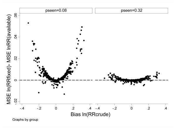
In the base case sensitivity analysis, simulation parameters were permuted to examine robustness of findings. In general, for scenarios in which there was little confounding (ie, bias RR_crude was low), the all-available and fixed window approaches performed similarly; for scenarios in which there was more confounding, MSE was lower for the all-available versus fixed window approach. Differences were more pronounced in scenarios in which pseen0 was lower (ie, in which C*_available and C*_fixed were discrepant [0.78 vs 0.39, respectively]), than in scenarios in which pseen0 was higher (ie, in which C*_available and C*_fixed were less discrepant [0.99 vs 0.90, respectively]) (Figure 2).

Figure 2.

Base case sensitivity findings. The difference in MSE for ln(RR_fixed) minus MSE ln(RR_available) is plotted versus bias for ln(RR_crude) under modeled scenarios where pseen0=0.08 and =0.32. Each point reflects estimates for one combination of simulation parameter values (as per Table 1). Positive values indicate better performance (ie, lower MSE) for the all-available approach.

Expanded model

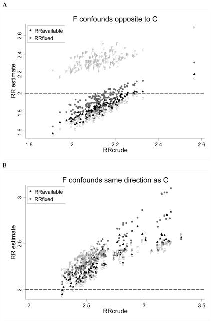
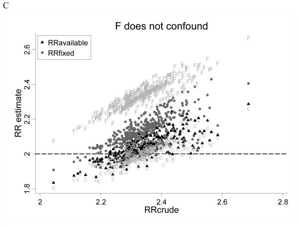
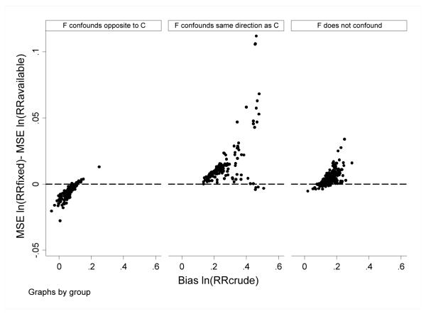
In the expanded model, we considered scenarios wherein subjects may differ in terms of an unmeasured confounder, which itself may be associated with C, and which may influence exposure status, coverage status, likelihood of medical contact and outcome (run to 4000 replicates). We evaluated bias according to permuted values of rref and rrdf and observed that when F did not confound the association between E and D (ie, rref=1 or rrdf=1) or when F confounded in the same direction as C (ie, rref and rrdf both >1, or both <1; because C confounds upwards), RR_available was consistently less biased than RR_fixed (Figure 3). When F confounded in the opposite direction as C (ie, rref>1 and rrdf<1, or vice versa), RR_fixed was less biased. In all instances, RR_available better approximated RR estimates that were adjusted for the true value of C; when F confounded in the direction opposite to C, RR_fixed was less biased than RR_available because there was greater residual (upward) confounding by C left to offset (downward) bias by F. As a result, MSE was lower for the all-available approach when F did not confound or when it confounded in the same direction as C, and was lower for the fixed window approach when F confounded in the opposite direction as C (Figure 4).

Figure 3.

Expanded case findings. RR risk estimates for the all-available (black triangles) and fixed window approaches (grey circles), estimates adjusted for the modeled value of C (“C”) and estimates adjusted for the modeled value of F (“F”) are plotted versus RR_crude. The modeled RR was 2.0 (dashed line). Each point reflects estimates for one combination of simulation parameter values (as per Table 1). Panel A considers scenarios where F confounds opposite to C (ie, rref>1 and rrdf<1, or rref<1 and rrdf>1). Panel B in considers scenarios where F confounds in the same direction as C (ie, rref>1 and rrdf>1, or rref<1 and rrdf<1). Panel C considers scenarios where F does not confound (ie, rref=1 and/or rrdf=1).

Figure 4.

Expanded case findings. The difference in MSE for ln(RR_fixed) minus MSE ln(RR_available) is plotted versus bias for ln(RR_crude). Each point reflects estimates for one combination of simulation parameter values (as per Table 1). Positive values indicate better performance (ie, lower MSE) for the all-available approach. The follow scenarios were considered separately: (left) F confounds opposite to C (ie, rref>1 and rrdf<1, or rref<1 and rrdf>1); (center) F confounds in the same direction as C (ie, rref>1 and rrdf>1, or rref<1 and rrdf<1); (right) F does not confound (ie, rref=1 and/or rrdf=1).

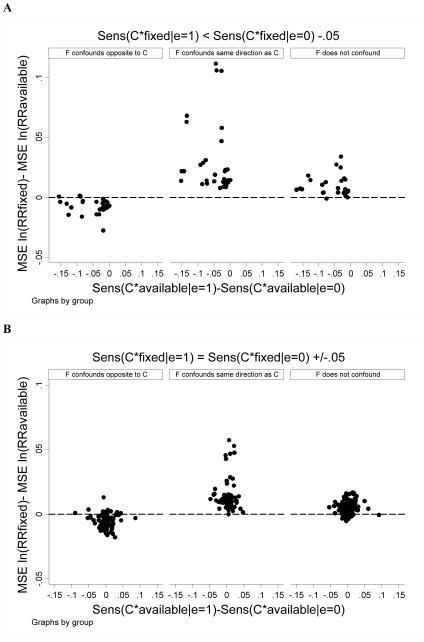
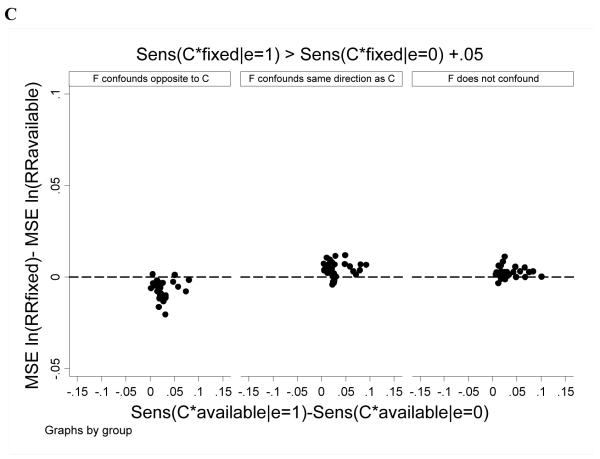
We examined whether differential sensitivity of C*_available and C*_fixed among exposed and unexposed subjects affected estimation. In general results were similar to those above: RR_available outperformed RR_fixed except in cases where F confounded in a direction opposite to C. This pattern was more accentuated when the sensitivity of C*_fixed was lower among exposed than unexposed subjects and when the sensitivity of C*_available was similar between exposed and unexposed subjects (Figure 5).

Figure 5.

Expanded case findings. The difference in MSE for ln(RR_fixed) minus MSE ln(RR_available) is plotted versus the difference in sensitivity of C*_available between exposed versus unexposed subjects. Each point reflects estimates for one combination of simulation parameter values (as per Table 1). Positive values indicate better performance (ie, lower MSE) for the all-available approach. Panel A considers scenarios where C*_fixed was 0.05 or more lower among exposed versus unexposed subjects. Panel B considers scenarios where C*_fixed was within 0.05 among exposed and unexposed subjects. Panel C considers scenarios where C*_fixed was 0.05 or more greater among exposed versus unexposed subjects.

To further explore the issue of differential sensitivity of C*, we manipulated simulation parameters such that C*_available was much more sensitive among exposed versus unexposed subjects, but the sensitivity of C*_fixed was similar across exposure groups. Among exposed subjects, median lead up time was 27.8 months, sensitivity C*_fixed was 0.39 and sensitivity of C*_available was 0.84; among unexposed subjects, median lead up time was 12.1 months, sensitivity of C*_fixed was 0.39 and sensitivity of C*_available was 0.62. Even in this circumstance, the pattern of association observed was similar to that seen in the expanded model (Table 3).

Table 3.

Extreme case results. Presented are RR estimates and MSE of ln(RR) for the crude, all-available and fixed window approaches. [Modeled RR=2; other simulation parameters: pc0=0.25; pe0=0.2; pd0=0.1; pf0=0.2; rrde=2; rrdc=2; rrec=2; pseen0=0.08; punenrolled0=0.12; rrfc=2; rruf=0.125; rrsf=1; rref=3; rrsu=1.]

	F and C confound in opposite directions (ie, rrdf=0.5)	F and C confound in the same direction (ie, rrdf=2)	F does not confound (ie, rrdf=1)
RR crude all-available fixed window	1.78 1.51 1.67	2.58 2.09 2.40	3.84 3.06 3.59
MSE crude all-available fixed window	0.02 0.08 0.04	0.07 0.004 0.03	0.43 0.18 0.34

DISCUSSION

In clinical medicine, the abbreviation WNL is used to designate a finding of “within normal limits” for a subject characteristic that might be assumed not to contribute to the clinical condition. If, however, the WNL abbreviation were taken to mean “we never looked,” then the measurement would be missing, potentially leading to an incorrect diagnosis. This concept could be applied to our designation of a binary confounder that is assumed not to be present unless a claim indicates it is. The occurrence of the claim is not only dependent on the presence of the condition for which it is a marker, but also on interaction with the healthcare system and coverage by the data capturing system. This uncertainty of covariate ascertainment even in the presence of disease suggests that improving sensitivity through extending baseline history, even if unequal across cohort members, has the potential to improve covariate capture and thereby confounder control.

Historical ascertainment is one aspect of misclassification. Specifically at issue is whether, in the setting of (possibly differential) misclassification inherent to the source data, deliberately inducing further misclassification (ie, through ignoring some of the available data) can lessen resultant bias. There is a robust literature regarding the impact of exposure (and outcome) misclassification on estimation. Non-differential exposure misclassification typically biases estimates toward the null.^{4, 6} Ergo in case—control studies, investigators often adhere to principle of comparable accuracy in assessing exposure to reduce the likelihood of observing spurious positive associations.⁷ Even toward this end, ensuring comparable accuracy is not a panacea, as the direction of bias becomes unpredictable when exposure misclassification is non-differential with respect to outcome,^{6, 8} or when exposure error is not independent of errors in other variables.^9-10 The situation becomes yet more complex when considering covariates, wherein even non-differential misclassification can bias unpredictably.^{4, 11-12} For these reasons, it cannot be assumed that comparable accuracy considerations logically extend to covariate ascertainment.

Through simulation studies, we tested whether, in situations in which subjects have differential amounts of lead-up time before exposure, dichotomous variables that are assumed to take on a value of zero in the absence of evidence to the contrary (eg, comorbid conditions) are better defined over all available lead-up time or over a fixed lead-up period common to all subjects. Our results indicate that use of all available lead-up data is less biased and yields a lower MSE than the fixed window approach in most cases.

In the base case scenario, we considered parameter values typical to what is seen in many large, claims based studies of patients with chronic medical conditions: moderate effects of confounder on exposure, confounder on outcome, and exposure on outcome (risk ratios=2); middling prevalences of exposure (20%) and confounder (25%); a per-month probability of uncoverage (4%) that corresponds to a mean available data window of 2 years; and a per-month likelihood of contact with the medical system (16%) that corresponds to a mean 1.8 visits/patient/year. In this case, consideration of confounder status over only the obligatory 6-month period common to all patients led to a parameter estimate that was 41% as biased as the crude estimate. Use of all available lead-up data led to a parameter estimate that was only 9% as biased as the crude estimate. When base case parameters were varied (within plausible ranges), it was observed that the all-available approach afforded better bias reduction and lower MSE in the setting of greater ambient confounding. Additionally, greater differences in estimation (favoring the all-available approach) were observed when the per-month probability of contact with the medical system was lower owing to implied differences in the sensitivity of C* under the two approaches.

We considered the possibility whereby an unmeasured covariate might influence the likelihood of exposure, outcome, data availability and contact with the medical system. For example, factors such as frailty may increase the likelihood of exposure (sicker patients needing more aggressive therapy) and outcome (sicker patients are sicker), factors such as exercise may decrease the likelihood of both, and factors such as substance abuse might decrease the likelihood of exposure (eg, less access to medical care¹³) while increasing the likelihood of outcome (eg, gastrointestinal bleeding¹⁴). In most scenarios, the all-available approach provided better estimation. The principal exception was that the fixed window approach was favored when an unmeasured covariate confounded the E—D association in the opposite direction as the measured confounder. In this situation, the benefits of the fixed window over the all-available approach stemmed from serendipitous counterbalancing of residual confounding from measured and unmeasured confounders: the net confounding from both factors was close to zero, so that controlling for one increased bias; because using all available data controlled for confounding on the basis of C more effectively than the fixed window approach, it resulted in more net bias. No situations were observed in which the fixed window (versus all-available) approach yielded estimates nearer the risk ratio adjusted for the true (modeled) value of C. We conclude that the optimal analytical response would therefore be to address sources of unmeasured confounding and then adjust maximally for all relevant confounding using the all-available approach. Beyond this, few scenarios were observed in which the fixed window approach was favored; even in these scenarios the fixed window approach was only modestly better than the all-available approach, whereas in other scenarios, much more substantive benefits of the all-available approach were observed.

These data cannot directly answer the question: how far back is far enough? However, inasmuch as the time periods considered here are relative (eg, months could equally be considered as calendar quarters or years, etc), there is no reason to suspect that there would be an upper bound on the historical time period that is potentially relevant. Instead, results indicate that more is typically better, and by extension, that all available data be leveraged (to the degree this can be feasibly implemented).

Some limitations of the study bear mention. First, the confounder considered here is one that is assumed to have a value of “normal” or “not present” in the absence of data to the contrary. Our results may not apply to variables for which missingness can be identified and corrective action taken (eg, imputation of missing quantitative covariates). Second, we cannot exclude the possibility that the fixed window approach would be favored under simulation conditions more extreme than those modeled; however, our simulation conditions attempted to encompass most situations that would be observed in applied research. Third, the confounder considered was assumed to be static over the period of study and to have time-invariant effects on exposure and outcome. Specifically, this assumption was based on a chronic disease conception, such as diabetes. We do not know whether these findings pertain to time-varying covariates, or those for which the effect on exposure or outcome has temporal dependence (eg, myocardial infarction). Fourth, use of longer minimum look-back periods to define new exposure will result in a smaller relative advantage of the all-available approach because it will reduce the amount of information to be added, although that apparent advantage comes at the cost of excluding more subjects who fail to meet the minimum look-back condition. Fifth, our findings pertain only to instances in which differential sensitivity of covariate definitions relate to historical lead-up windows. Specifically, consideration of historical lead-up windows impose two important restraints on the data that may not pertain to other situations in which comparable accuracy of covariate definitions is at question: 1) the sensitivity of C* under the fixed widow approach cannot exceed that of the all-available approach, and 2) extreme differences in the sensitivity of C* between exposed and unexposed groups under the two approaches are mitigated because subjects with dramatically short historical data windows are dropped from the analysis due to less than requisite lead-up time. Finally, our data pertain only to estimates pooled across C and does not address heterogeneity of estimates across strata of C as observed in other circumstances.¹¹

In summary, this simulation study supports using all available historical data rather than data observed over a historical window commonly shared by all subjects to define time-invariant dichotomous covariates in most circumstances.

Glossary

C

measured covariate

C*

value of measured covariate considered analytically

D

disease (outcome)

E

exposure

F

unmeasured covariate

pc

marginal probability that measured covariate =1

pd0

conditional probability that outcome=1 given exposure=0 and measured covariate =0^≠

pe0

conditional probability that exposure =1 given measured covariate=0^≠

pseen0

per month likelihood of contact with the healthcare system^≠

punenrolled0

per month likelihood of that a given month was the historically most recent month for which the subject was not represented in source data^≠

RR

risk ratio

rrdc

risk ratio of measured covariate on outcome

rrde

risk ratio of exposure on outcome

rrdf

risk ratio of unmeasured covariate on outcome

rrec

risk ratio of measured covariate on exposure

rref

risk ratio of unmeasured covariate on exposure

rrfc

risk ratio of measured covariate on unmeasured covariate

rruf

risk ratio of unmeasured covariate on data availability

rrsf

risk ratio of unmeasured covariate on likelihood of medical contact

References

- 1.Fisher ES, Whaley FS, Krushat WM, et al. The accuracy of Medicare’s hospital claims data: progress has been made, but problems remain. Am J Public Health. 1992;82:243–8. doi: 10.2105/ajph.82.2.243. [DOI] [PMC free article] [PubMed] [Google Scholar]
- 2.Tagalakis V, Kahn SR. Determining the test characteristics of claims-based diagnostic codes for the diagnosis of venous thromboembolism in a medical service claims database. Pharmacoepidemiol Drug Saf. 2011;20:304–7. doi: 10.1002/pds.2061. [DOI] [PubMed] [Google Scholar]
- 3.Savitz DA, Baron AE. Estimating and correcting for confounder misclassification. Am J Epidemiol. 1989;129:1062–71. doi: 10.1093/oxfordjournals.aje.a115210. [DOI] [PubMed] [Google Scholar]
- 4.Greenland S. The effect of misclassification in the presence of covariates. Am J Epidemiol. 1980;112:564–9. doi: 10.1093/oxfordjournals.aje.a113025. [DOI] [PubMed] [Google Scholar]
- 5.Sox CM, Swartz K, Burstin HR, Brennan TA. Insurance or a regular physician: which is the most powerful predictor of health care? Am J Public Health. 1998;88:364–70. doi: 10.2105/ajph.88.3.364. [DOI] [PMC free article] [PubMed] [Google Scholar]
- 6.Flegal KM, Keyl PM, Nieto FJ. Differential misclassification arising from nondifferential errors in exposure measurement. Am J Epidemiol. 1991;134:1233–44. doi: 10.1093/oxfordjournals.aje.a116026. [DOI] [PubMed] [Google Scholar]
- 7.Wacholder S, McLaughlin JK, Silverman DT, Mandel JS. Selection of controls in case-control studies. I. Principles. Am J Epidemiol. 1992;135:1019–28. doi: 10.1093/oxfordjournals.aje.a116396. [DOI] [PubMed] [Google Scholar]
- 8.Brenner H, Loomis D. Varied forms of bias due to nondifferential error in measuring exposure. Epidemiology. 1994;5:510–7. [PubMed] [Google Scholar]
- 9.Chavance M, Dellatolas G, Lellouch J. Correlated nondifferential misclassifications of disease and exposure: application to a cross-sectional study of the relation between handedness and immune disorders. Int J Epidemiol. 1992;21:537–46. doi: 10.1093/ije/21.3.537. [DOI] [PubMed] [Google Scholar]
- 10.Kristensen P. Bias from nondifferential but dependent misclassification of exposure and outcome. Epidemiology. 1992;3:210–5. doi: 10.1097/00001648-199205000-00005. [DOI] [PubMed] [Google Scholar]
- 11.Walker AM, Lanes SF. Misclassification of covariates. Stat Med. 1991;10:1181–96. doi: 10.1002/sim.4780100803. [DOI] [PubMed] [Google Scholar]
- 12.Gustafson P, Le Nhu D. Comparing the effects of continuous and discrete covariate mismeasurement, with emphasis on the dichotomization of mismeasured predictors. Biometrics. 2002;58:878–87. doi: 10.1111/j.0006-341x.2002.00878.x. [DOI] [PubMed] [Google Scholar]
- 13.Weissman G, Melchior L, Huba G, et al. Women living with substance abuse and HIV disease: medical care access issues. J Am Med Womens Assoc. 1995;50:115–20. [PubMed] [Google Scholar]
- 14.Schauer DP, Moomaw CJ, Wess M, Webb T, Eckman MH. Psychosocial risk factors for adverse outcomes in patients with nonvalvular atrial fibrillation receiving warfarin. J Gen Intern Med. 2005;20:1114–9. doi: 10.1111/j.1525-1497.2005.0242.x. [DOI] [PMC free article] [PubMed] [Google Scholar]