Quantitative analysis of DNA looping kinetics from tethered particle motion experiments

Abstract

In this chapter we show the application of a maximum likelihood-based method to the reconstruction of DNA looping single-molecule time traces from tethered particle motion experiments. The method does not require time filtering of the data and improves the time resolution by an order of magnitude with respect to the threshold-crossing approach. Moreover, it is not based on presumed kinetic models, overcoming the limitations of other approaches proposed previously, and allowing its applications to mechanisms with complex kinetic schemes. Numerical simulations have been used to test the performances of this analysis over a wide range of time scales. We have then applied this method to determine the looping kinetics of a well-known DNA-looping protein, the λ-repressor CI.

1. Introduction

Transcription regulation of many genes occurs via DNA looping, which brings into close proximity proteins bound at distant sites along the double helix. Looping produces shortening of the DNA molecule and activation or repression (depending on the gene and proteins involved) of promoters in the loop region.

By means of the tethered particle motion (TPM) technique, changes in the conformation of DNA molecules can be indirectly monitored in vitro at the single molecule level, by observing the diffusion of a sub-micron-sized bead tethered to the surface of a microscope coverslip by single DNA molecules (Finzi and Dunlap, 2003; Finzi and Gelles, 1995; Gelles et al., 1995; Pouget et al., 2004; van den Broek et al., 2006; Vanzi et al., 2006; Yin et al., 1994; Zurla et al., 2006; Zurla et al., 2009; Zurla et al., 2007). In a typical TPM experiment, the molecule is attached with one end to a glass slide and with the other to a sub- micron-sized particle. As schematically depicted in Fig. 1, the measurement of the particle position is used to determine changes in DNA conformation, such as looping due to specific protein binding.

Figure 1.

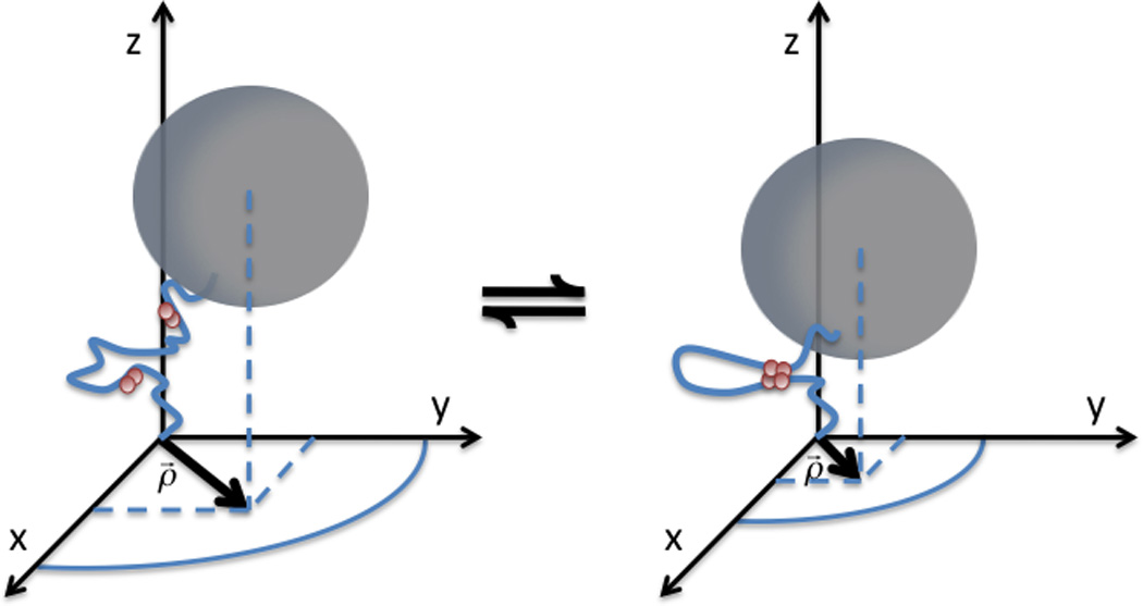
Schematic representation of the looping mechanism. Proteins bound at distant sites along the DNA can interact establishing a DNA loop. The loop shortens the DNA, reducing the range of diffusion of the tethered bead.

Due to the Brownian diffusion of the particle and the overlap between the looped and unlooped distributions, the determination of the dynamic changes usually requires time filtering of the raw data, significantly impacting the measurement time resolution and the reliability of the determination of the kinetic constants. Methods have been proposed to either correct for such a drawback (Colquhoun and Sigworth, 1983; van den Broek et al., 2006; Vanzi et al., 2006) or determine the kinetic constants from the raw data (Beausang et al., 2007a; Beausang et al., 2007c; Qin et al., 2000). Nevertheless, these approaches require the knowledge of the kinetic mechanism of the reaction being considered and their application is limited to fairly simple reaction schemes.

In this chapter we describe the successful application to TPM experiments of a maximum-likelihood method, previously used for the detection of changes in diffusion coefficients (Montiel et al., 2006) of a freely diffusing particle and in the intensity of fluorescence resonance energy transfer signals (Watkins and Yang, 2005). As tested by analysis of simulated data, this method allows for the reconstruction of the looping kinetics without time filtering at increased time resolution (~200 ms) with respect to the general half-amplitude threshold approach (Colquhoun and Sigworth, 1983; van den Broek et al., 2006; Vanzi et al., 2006), which is customarily used to analyze this kind of experimental data.

2. Change point algorithm

The change point (CP) algorithm is a maximum-likelihood, ratio-type statistical approach for testing a sequence of observations for no change in a given parameter against a possible change, while other parameters remain constant (Gombay, 1996; Watkins and Yang, 2005). Here, we discuss its application to the time series of a scalar random variable x_i (which represents the observable of a measurement) with i being a discrete time index. We assume that the probability distribution of the variable is f (x_i;σ), where σ is a one-dimensional parameter. The extension of this problem to higher dimensionality cases for both the random variable and the distribution parameter can be found in (Gombay, 1996).

The log-likelihood function for observing a set of N values of x_i is calculated as:

$$g(x_i;\sigma )=\text{log}(\prod _{i=1}^{N}f(x_i;\sigma ))=\sum _{i=1}^N\text{log}(f(x_i;\sigma ))$$ (1)

By the maximization of the log-likelihood function, the maximum likelihood estimator σ̂ can be derived.

To assess the presence of a change point in the parameter σ for a given index k, the null hypothesis:

$$H_0:\sigma (1)=\dots =\sigma (k)=\sigma (k+1)=\dots =\sigma (N),$$ (2)

must be compared with the change point hypothesis:

$$H_{CP}:\sigma (1)=\dots =\sigma (k)={\sigma }_1\ne {\sigma }_2=\sigma (k+1)=\dots =\sigma (N)$$ (3)

The test between the two hypotheses can be executed via the calculation of the log-likelihood ratio:

$$R(k)=\text{log}\left(\frac{f(x_{1,\dots ,k};{\mathrm{\sigma ̂}}_1)f(x_{k+1,\dots ,N};{\mathrm{\sigma ̂}}_2)}{f(x_{1,\dots ,N};\mathrm{\sigma ̂})}\right)=g(x_{1,\dots ,k};{\mathrm{\sigma ̂}}_1)+g(x_{k+1,\dots ,N};{\mathrm{\sigma ̂}}_2)-g(x_{1,\dots ,N};\mathrm{\sigma ̂}),$$ (4)

which represents a measure of the likelihood to have a change point at k.

Since in our problem the location of the change point is unknown, we first need to calculate the position at which the occurrence of a change point is most likely to occur. This can be easily calculated as the index $i^{*}=\text{arg}\{\underset{1<k<N}{\text{max}}(R(k))\}$.

The problem, then, is the quantification of how large has R(i^*) to be in order for the hypothesis H₀ to be rejected with a given level of confidence or, in other words, to establish a threshold which allows assessment of the presence of the change point with a known probability.

If we define:

$$Z_N=\underset{1<k<N}{\text{max}}(2R(k))=2R(i^{*}),$$ (5)

the problem of the change point identification can be reformulated as:

$$\{\begin{array}{c}{Z}_N\ge C_{1-\alpha }\to H_0\text{is rejected}\hfill \\ Z_N<C_{1-\alpha }\to H_0\text{is accepted}\hfill \end{array}$$ (6)

where C_1−α is intrinsically defined by:

$$\text{Probability}(Z_N\ge C_{1-\alpha })=1-\alpha ,$$ (7)

with α being the probability of having a false-positive change point (Type-I error).

The calculation of C_1−α requires the knowledge of the distribution of Z_N. Although this distribution has not been calculated in closed form, its approximations and their rate of convergence have been extensively studied (Gombay, 1996 and references therein).

In particular, it has been found that the limiting distribution of Z_N can be approximated by the distribution of another random variable, which has been derived in closed form (Gombay, 1996). To test for a change point in the value of a one-dimensional parameter, this distribution is given by (Vostrikova, 1981):

$$\frac{\sqrt{C_{1-\alpha }}\text{exp}(-C_{1-\alpha }/2)}{\sqrt{2}\mathrm{\Gamma }(\frac{1}{2})}\{T-\frac{1}{C_{1-\alpha }}T+\frac{4}{C_{1-\alpha }}\}=1-\alpha$$ (8)

where: $T=\text{log}\left(\frac{{(1-h)}^2}{h^2}\right),h=\frac{{(\text{log}N)}^{3/2}}{N}$ and Γ is the gamma function.

Numerical solution of the equations above allows determination of the asymptotic critical values for type-I error rates. Although these values are a conservative estimate for C_1−α, in cases where the exact knowledge of the type-I error is not strictly required, their use offers the advantage of a fast calculation, while otherwise the calculation of the critical region needs to be performed numerically (Serge et al., 2008; Watkins and Yang, 2005).

3. Data clustering and expectation-maximization (EM) algorithm

Once the change points have been determined by the CP algorithm described in the previous section, in the many cases where the changes in the parameter σ occur among several levels, it is necessary to refine the previous analysis by clustering the change-point regions in states. Under the hypothesis that the number of states S (i.e. the levels of the parameter σ) is known, it is possible to perform this refinement by means of hierarchical clustering of the data (Fraley and Raftery, 2002).

Such an approach consists of defining a “distance” between the change-point regions. This distance is then calculated between every pair of regions and, according to its value, the regions are grouped in a hierarchical tree. After this classification, the data can be partitioned into the S states by means of a grouping criterion. Nevertheless, this kind of clustering is highly sensitive to initial conditions. To overcome this problem, Watkins and Yang (Watkins and Yang, 2005), following (Fraley and Raftery, 1998; Fraley and Raftery, 2002), proposed to use the result of this procedure as initial guess for more advanced analysis based on an expectation-maximization (EM) algorithm (Dempster et al., 1977; Fraley and Raftery, 1998; Fraley and Raftery, 2002).

This can be understood considering the following. Let us suppose that, from the change-point analysis, M change points are detected. This results in having M−1 change-point regions, each with a given maximum likelihood estimator σ̂_m. For the hierarchical clustering of these M−1 regions in S state, consistently with Eq. (4), a “metric-like” function between two change-point regions can be defined as:

$$d(m_1,m_2)=g(\{x_{m1}\};{\mathrm{\sigma ̂}}_{m1})+g(\{x_{m2}\};{\mathrm{\sigma ̂}}_{m2})-g(\{x_{m1}\cup x_{m2}\};{\mathrm{\sigma ̂}}_{m1\cup m2})$$ (9)

where m₁,m₂ = 1,…,M −1 (Scott and Symons, 1971). The so-defined matrix represents indeed a “distance” between two regions in the maximum likelihood sense.

Recursively, the two regions having the smallest “distance” are grouped until S clusters are finally formed. According to this procedure, a matrix p(m,s) with m = 1,…,M −1 and s = 1,…,S identifies whether the m^th region has been assigned to the s^th cluster (p(m,s) = 1) or not (p(m,s) = 0).

Once the hierarchical clustering has provided the initial conditions, the clustering refinement proceeds through the expectation-maximization routine. The two steps of this algorithm consist in an expectation step, in which the matrix p(m,s) is updated on the basis of the parameters calculated in the previous step, and a maximization step in which the total likelihood function is maximized. The two steps are repeated until p(m,s) converges.

The total log-likelihood function is given by:

$$L=\sum _{m=1}^{M-1}\sum _{s=1}^{S}p(m,s)\text{log}\{p_{s}g(\{x_m\};{\sigma }_s)\},$$ (10)

where p_s represents the relative weight of each state in the mixture.

4. Adaptation of the method to the case of TPM data analysis

The output of a TPM measurement is a time series of the center position (x(t),y(t)) of the tethered bead (Zurla et al., 2006). Since the probability distribution of x(t)and y(t) depends on the DNA tether length (Nelson et al., 2006), changes in such distribution, observed in the presence of a DNA-looping protein, can be indirectly related to changes in the DNA looping state, providing the possibility to characterize the dynamics of DNA loop formation and breakdown in vitro (Figure 2).

Figure 2.

Time traces of x(t), y(t) and ρ(t) for a 240 nm-radius bead tethered to an unlooped (length 3477 bp) and looped (effective length 1160 bp) DNA molecule, and corresponding probability distributions. The distribution histogram of x(t) and y(t) deviates from a Gaussian behavior (red curves) due to the excluded-volume effect given by the finite size of the bead. Similarly, the histogram of ρ(t) shows a discrepancy with respect to the Rayleigh distribution (red curve) but is instead well described by a two-parameter Weibull distribution (in black). Histograms have been normalized to the bin width w (w=30 nm) and to the total number of data points n (n = 30000).

The CP-EM method described in the previous section was applied to identify changes in the looping state of single DNA molecules. A Gaussian distribution was assumed for the probability density function, pdf, of the time series of x(t) and y(t):

$$f_{TPM}(x_i;{\sigma }_x)=\frac{1}{\sqrt{2\pi {\sigma }_x^2}}\text{exp}\{-\frac{x_i^2}{2{\sigma }_x^2}\}.$$ (11)

It must be noted that the pdf for x(t) and y(t) (Fig. 2) deviates from a Gaussian distribution, as expected from the Worm-Like Chain model in the entropic regime (Qian, 2000; Qian and Elson, 1999), because the finite size of the bead causes an excluded volume effect (Nelson et al., 2006; Segall et al., 2006). The exact distribution of x(t) and y(t) has been calculated through Monte Carlo integration of the Boltzmann distribution (Segall et al., 2006), but an analytical expression for such a distribution has not been derived. Although in principle a parametric expression for the pdf can be calculated from the Pearson system of distributions, based on the knowledge of its first four moments, and the calculation of the maximum-likelihood estimator can be numerically performed via maximization of the likelihood function, this approach critically affects the computational time of the change point determination. Therefore, at this stage, an analytical calculation based on the Gaussian approximation is preferable. By contrast, a numerical approach was used in the expectation-maximization step, where the shape of the distribution significantly affects the determination of the looping dynamics.

According to the previous equation, the log-likelihood of observing N displacement is given by:

$$g_{TPM}(x_i;\sigma )=\text{log}\left[\prod _{i=1}^N\frac{1}{\sqrt{2\pi {\sigma }_x^2}}\text{exp}\right\{-\frac{x_i^2}{2{\sigma }_x^2}\left\}\right]=-\frac{N}{2}\text{log}(2\pi {\sigma }_x^2)-\frac{1}{2{\sigma }_x^2}\sum _{i=1}^N{x}_i^2.$$ (12)

Maximization of the latter equation provides the expression for the maximum-likelihood estimator ${\mathrm{\sigma ̂}}_x^2=\frac{1}{N}\sum _{i=1}^N{x}_i^2$.

The log-likelihood ratio for the detection of a change point is then calculated as:

$$R_{TPM}^{(x)}(k)=-\frac{k}{2}\text{log}\left(\sum _{i=1}^k{x}_i^2\right)-\frac{N-k}{2}\text{log}\left(\sum _{i=k+1}^N{x}_i^2\right)+\frac{N}{2}\text{log}\left(\sum _{i=1}^N{x}_i^2\right)+\dots +\frac{k}{2}\text{log}(k)+\frac{N-k}{2}\text{log}(N-k)-\frac{N}{2}\text{log}(N).$$ (13)

The search for change points in a TPM measurement is performed using a segmentation algorithm, similarly as described in (Watkins and Yang, 2005). The time series x(t) and y(t) are segmented in traces of N=1000 points (200 s) each, with a partial overlap of 500 points. As a matter of fact, the error in the detection of a change point depends on its position and has maxima at the edges of the segment and reaches its minimum at the middle point (Watkins and Yang, 2005). The overlap between consecutive fragments thus ensures a nearly constant error rate for all change points. After the segmentation, the maximum of $R_{TPM}(k)=R_{TPM}^{(x)}(k)+R_{TPM}^{(y)}(k)$ is calculated over the segment and, if it is greater or equal to $C_{1-\alpha }^{\mathit{\text{sim}}}$, the associated index is identified as a change point.

The change point determination routine is schematically represented in Fig. 3. This procedure is then repeated over the two distinct fragments divided by the determined change point and recursively applied for each detected change point, until no further change points are found. After the procedure is completed over a segment, each change point position is refined by the re-application of the algorithm mentioned above to a segment defined by its two nearest-neighboring change points.

Figure 3.

Change point determination. Simulated traces for a DNA molecule showing a looping event for k = 500 (t = 10s). The time dependence of the bead center position x(t) and y(t) is reported in the two upper panels respectively. In the third panel, the log-likelihood ratio R_TPM (k) is plotted as a function of k. The red dot-dashed line represents the critical value (α = .99, N = 1000) for the change point detection. The maximum of R_TPM is found for k = i^* = 498. The bottom panel shows the plot of the radial distance of the bead center $\rho (t)=\sqrt{x^2(t)+y^2(t)}$. The “true” trace is also displayed (black line) for comparison.

Calculation of the critical regions $C_{1-\alpha }^{\mathit{\text{sim}}}$ is obtained via numerical simulations. For each k ranging from 2 to 1000, 10000 traces presenting no change point were simulated for x(t) and y(t) from a Pearson-type distribution having the same first four moments as the experimental data. From the traces, the distribution of max(R_TPM(k)) was then calculated, allowing the determination of the critical region for each level of confidence (Fig. 4). A similar calculation, based on simulated traces presenting a change point, also allows one to obtain the probability of missed events (Fig. 4, dot-dashed lines).

Figure 4.

Critical regions $C_{1-\alpha }^{\mathit{\text{sim}}}$ (continuous lines) obtained by numerical simulations as a function of N for several level of the confidence interval α for the false-positive event determination. The dependence on N of the critical value for the probability of missed events is reported as dot-dashed lines. Note that at a 31% (α=.69) confidence level for false positive event the probability of missing the detection of a change point occurring in a region of N≥50 data points (t≥1s) is smaller than 10%.

The change point determination is then followed by the expectation-maximization routine, schematically represented in Fig. 5. As previously stated, at this step the exact knowledge or a good approximation of the shape of the experimental pdf is highly critical for proper clustering of the change point regions. The deviation of the distribution of x(t) and y(t) from a normal pdf does not allow one to use the Gaussian approximation. Nevertheless, through the calculation of its first four moments, the pdf of x(t) and y(t) can be associated with a Pearson type II distribution and thus approximated to a scaled symmetrical Beta distribution. The maximization of the associated likelihood function can, in principle, be computed numerically. Unfortunately, since the Beta distribution is defined on the interval [0,1] and the scaling factor is used as one of the parameters of the maximization, the numerical optimization is made non-trivial by the fact that data points can lie outside the range of definition of the function.

Figure 5.

Expectation-maximization clustering.

Left panel. After the change points have been determined (black crosses), the regions between two adjacent change points are clustered into two groups through the maximization of the total log-likelihood function for a Weibull pdf. The green and red lines represent the average of the data points in the corresponding change point region. The color identifies the DNA conformation corresponding to the two groups (red-unlooped and green looped). The “true” trace (black line) is also reported shifted and scaled for comparison. Right panel. Histogram of the time trace and results of the expectation-maximization step. The red and green curves refer to the retrieved Weibull pdf for the unlooped and looped state, respectively. The sum of the two probability density functions (black line) shows an excellent agreement with the data histogram.

Although the probability distribution of $\rho (t)=\sqrt{x^2(t)+y^2(t)}$ it is also a Beta-like distribution (Pearson type I distribution), it can be well approximated by the two-parameters Weibull function:

$$f_{WBL}(\rho ;a,b)=b{a}^{-b}{\rho }^{b-1}\text{exp}\{-{\left(\frac{\rho }{a}\right)}^b\},$$ (14)

which is defined over the positive real axis and for which the numerical maximization of the likelihood function can be easily performed.

It is worth noting that, for b = 2, the Weibull pdf reduces to the well known Rayleigh function, the distribution function for the modulus of a vector having its two orthogonal components independent and normally distributed. For a Rayleigh pdf the maximum likelihood estimator is moreover given by $â=\sqrt{\frac{\sum _{i=1}^N{\rho }_i^2}{N}}$, which is the quantity usually calculated over a given window size in the threshold method (Nelson et al., 2006; Zurla et al., 2006).

Hierarchical clustering of the change point regions in S=2 states (unlooped and looped) is thus carried out through the recursive calculation of the metric-like matrix:

$$d(m_1,m_2)=g_{WBL}(\{{\rho }_{m1}\};{â}_{m1},{\mathrm{b̂}}_{m1})+g_{WBL}(\{{\rho }_{m2}\};{â}_{m2},{\mathrm{b̂}}_{m2})+\dots -g_{WBL}(\{{\rho }_{m1}\cup {\rho }_{m2}\};{â}_{m1\cup m2},{\mathrm{b̂}}_{m1\cup m2}),$$ (15)

where g_WBL (ρ;a,b) is now defined as:

$$g_{WBL}(\rho ;a,b)=\text{log}\left(\prod _{i=1}^{N}b{a}^{-b}{\rho }_i^{b-1}\text{exp}\right\{-{\left(\frac{{\rho }_i}{a}\right)}^b\left\}\right)$$ (16)

and the maximum likelihood estimators â and b̂ are obtained through numerical maximization.

The results of the clustering are then used as a first guess for the expectation-maximization step, which proceeds in this case to the calculation of the matrix p(m,s) via the numerical maximization of the global log-likelihood function:

$$L_{WBL}=\sum _{m=1}^{M-1}\sum _{s=1}^{S}p(m,s)\text{log}\{p_s{g}_{WBL}(\{{\rho }_m\};a_s,b_s)\}.$$ (17)

5. Performance of the method

Although the rate of false positive identification and the probability of missed events for the detection of a change point can be easily calculated depending on the position of the change point and length of the trajectory, this is not straightforward when dealing with trajectories showing a series of change points. In this case, the dependence of the probability of detection and the error on the duration of the change point region are also affected by the probability of detection of the neighboring change points. Intuitively, the power of detection for a change point region depends on its length, i.e. on the time the trace dwells in a given state. On the other hand, the error of the calculation of the dwell time also depends on the accuracy at which the contiguous regions are determined and assigned to the “true” state. In order to estimate how the detection probability varies with the dwell time we used a simplified approach, based on numerical simulations. In particular, traces showing transitions between the looped and unlooped states with randomly distributed dwell times were generated and analyzed as described in the previous section. The ratio between the number of detected (n) and simulated (n_s) dwell times with durations lying in windows of exponentially increasing widths was then plotted and considered as an estimate of the power of detection of the method. Fig. 6 shows the values of n/n_s as obtained at a 31% false-positive detection rate $(C_{1-.69}^{\mathit{\text{sim}}})$ for the loop and the unloop state as a function of the dwell time. Although the curves intersect at a dwell time of ~ 0.8 s with 60% of the events detected, the plot shows an asymmetry between the detection abilities of the loop and the unloop states. This is most likely due to the expectation-maximization step during which, because of the large overlapping area between the Weibull pdf’s, short-lived regions have higher probability to be attributed to the unlooped distribution. It must be noted that these simulations provide just an estimate of the power of detection. In this case no attempt has been made to determine the confidence level for false-positive and missed-event probabilities, as a more rigorous approach would require. Therefore, the results shown in Fig. 6 could be partially biased by some sort of compensation between false-determined and missed events.

Figure 6.

Log-log plot of the ratio between the number of detected and the number of simulated change point regions as a function of the dwell time duration.

To further check for the ability of the method to detect DNA transitions between looped and unlooped states in the traces obtained from TPM experiments, time traces were simulated in which the dwell times spent in the two configurations are exponentially distributed with mean lifetimes τ_L and τ_U ranging from 1 s to 1 min. For each case, 20 traces with a duration of each 20 min were generated and analyzed. As already mentioned, actual TPM experimental data show correlation in the bead position that is not present in the simulated trace. The time scale of this correlation is of the order of hundreds of milliseconds for a ~250 nm radius bead tethered to a roughly micron long DNA (Beausang et al., 2007a; Beausang et al., 2007b; Beausang et al., 2007c). To prevent this correlation from increasing the number of false-positive events shorter than its decay time and inducing a bias in the change point determination, it is necessary to consider only events larger than the correlation time. Although the simulated data do not present this kind of correlation, for sake of consistency only dwell times longer than T_D = 200 ms were kept and the mean lifetimes were calculated through the maximization of the likelihood function for the exponential distribution: $f=\frac{1}{\tau }\text{exp}\{-\frac{t-T_D}{\tau }\}$.

All lifetimes obtained are reported on the log-log plot of Fig. 7 together with the “true” values τ^true as obtained from the simulated traces. The plot shows that although the ability to detect dwell times is affected by the average duration of both states, the method allows for the determination of even very small lifetimes with considerable accuracy. The contour map of the average relative error $\mathrm{\Delta }({\tau }_U^{\mathit{\text{true}}},{\tau }_L^{\mathit{\text{true}}})=\frac{1}{2}[\frac{|{\tau }_U^{\mathit{\text{true}}}-{\mathrm{\tau ̂}}_U|}{{\tau }_U^{\mathit{\text{true}}}}+\frac{|{\tau }_L^{\mathit{\text{true}}}-{\mathrm{\tau ̂}}_L|}{{\tau }_L^{\mathit{\text{true}}}}]$ shows indeed a flat region with values of Δ < 0.2, with partial degradation of the accuracy at the left and bottom edges. Moreover, consistent with what we previously noted, in this case also an asymmetry between the accuracy in the determination of looped and unlooped lifetimes is observed.

Figure 7.

Comparison among loop and unloop lifetimes used to generate the simulated time traces (crosses) and the values (filled circles) determined by means of the CP-EM (upper-left panel) and the HAT method (upper-right panel).

The lower panels show the contour plots of the average relative error Δ on the loop and unloop lifetimes retrieved using the CP-EM (left) and the HAT (right) method, with respect to the “true” lifetime values used in the simulations. The white line, delimiting the contour region corresponding to Δ=0.5, is reported in both the plots for comparison.

In Fig. 8, the histograms of the recovered dwell times for the case τ_U = 8 s, τ_L = 4 s are plotted together with the distribution of the “true” times generated via the simulation (left panels). From the histograms, it is possible to see that the method preserves the exponential shape of the dwell time distribution. As expected, the number of missed events decreased with the dwell times duration, reaching ~10% for values shorter than the mean lifetime and thus allowing for a precise determination of the decay constant. Moreover, short-lived missed events do not induce any relevant alteration of the shape of the distribution at larger dwell times through the creation of false long-lived states.

Figure 8.

Comparison between CP-EM and HAT method on simulated data. In the upper panels a representative part of a simulated trace (τ_U = 4 s, τ_L = 8 s) is shown together with the reconstructed telegraphic-like behavior (black lines) obtained by means of the CP-EM (left) and the HAT (right) method. The “true” signal is also shown (red lines) scaled and shifted for comparison. The improved CP-EM time resolution allows a better reconstruction of the trajectory, permitting the detection of short dwell times.

Middle panels. Histograms of the unlooped dwell times as retrieved by the CP-EM (left) and HAT (right) method for a simulated experiment (τ_U = 4 s, τ_L = 8 s). The red line represent the histogram of the “true” simulated unlooped dwell time and the black line is the exponential fit to the retrieved data.

Bottom panels. Same plot as above for the looped dwell times.

From the histograms it is clear that the CP-EM allows the determination of the mean lifetime for the simulated data with high accuracy with respect to the HAT method, owing to its higher time resolution and the lower number of short-lived missed events.

6. Comparison with the threshold method

A common approach to the analysis of TPM data is the half-amplitude threshold method (HAT). This approach relies on the time filtering of the ρ² time trace with a rectangular or Gaussian filter of given width. This allows for the calculation of the square root of the signal variance $\sqrt{{\langle {\rho }^2\rangle }_W}$ (weighted in the case of Gaussian filter) over the time trace. In the case of DNA showing looping transitions, this procedure requires that clearly visible steps emerge in the data. The histogram of the filtered data shows indeed a bimodal distribution, which allows defining a threshold as the half amplitude between the means of the two distribution peaks. The threshold, as well as the distribution of $\sqrt{{\langle {\rho }^2\rangle }_W}$, depends on the filter width. The dwell times are then obtained from the threshold crossing points of the filtered data. The width of the filter determines the time resolution of the analysis. This is expressed as the dead time, i.e. the duration of a loop (or unloop) event that after filtering gives a half-amplitude response (for a rectangular filter, the dead time corresponds to half of the window width) (Colquhoun and Sigworth, 1983). Events with a time duration below the dead time are then neglected in the dwell time calculation. It must be noted that there is no uniform criterion for the choice of an optimal filter. As a rule of thumb, the filter width should be the smallest possible (at least shorter than the minimum lifetime) that still allows for a clear identification of the loop and unloop events from the distribution histogram.

On the other end, as already pointed out, there is another factor to take into account, which is the time scale for the bead to traverse its range of motion. As discussed in (Beausang et al., 2007a; Beausang et al., 2007c), this induces a correlation in the bead’s position and limits the choice of the filter width. As a consequence, relatively large filter widths must be used (~4 s), resulting in rather poor time resolution.

Nevertheless, several methods have been proposed to correct for missed events by the use of several filter widths (Vanzi et al., 2006), by bypassing the time-filtering step through the Hidden Markov method (Qin et al., 2000), or by taking into account the diffusion of the bead (Beausang et al., 2007a; Beausang et al., 2007c).

Unfortunately, in all of these cases, the knowledge of the kinetic reaction scheme is crucial to obtain the correct value for the rate constant. This makes these methods extremely difficult to apply when dealing with complex kinetic schemes. For the change-point expectation-maximization method (CP-EM), this information is not required since the dwell time distribution is retrieved without any assumption on the kinetics of the system. Moreover, once the dwell time distribution has been determined with high time resolution, if necessary other methods (Liao et al., 2007) can be applied to resolve complex kinetics and determine the rate constants.

Our CP-EM is a maximum likelihood method for the reconstruction of the “true” time traces with high temporal resolution. Its performance was compared with the half-amplitude threshold approach. A direct comparison was performed by applying the HAT method also to the simulated data of the previous section. In the HAT case we used a rectangular filter of width W= 4s (200 data points) (Nelson et al., 2006; Zurla et al., 2006). In the threshold analysis, only dwell times longer than the dead time (2 s) were retained and the calculation of the mean lifetime was performed through the maximization of the log-likelihood function for an exponential pdf on times larger than twice the dead time (Colquhoun and Sakmann, 1981; Colquhoun and Sigworth, 1983). The results of the analysis performed by the HAT method on the simulated traces are reported in the panels on the right of Figs. 7 and 8. The calculated lifetimes largely deviate from the “true” values for τ’s shorter than 10 s and, even for larger τ’s, the relative error is about one order of magnitude larger than when using the CP-EM (Fig. 7). The high cutoff imposed by the time filtering limits the resolution, causing a large number of missed events at short times that in turn induce the detection of false long-lived states (Fig. 8), artificially increasing the determined lifetime.

7. Application to TPM experiments: CI-induced looping in λ DNA

The CI induced looping in λ-DNA has been recently proposed as the mechanism by which the λ epigenetic switch is regulated (Dodd et al., 2001). Looping strengthens repression of the lytic genes during lysogeny, while simultaneously controlling CI concentration, thus ensuring an efficient switch to lysis. This looping is achieved via the interaction of up to six CI dimers with two DNA regions, containing three binding sites each and separated by 2317 base pairs (bp). According to recent studies (Anderson and Yang, 2008; Dodd et al., 2004; Zurla et al., 2009), the number of CI dimers involved in the loop closure plays a major role in switch regulation, by affecting the stability of the long-range interaction.

Therefore, a detailed understanding of the looping kinetics of the CI-mediated switch is necessary as underpinning for its regulatory function.

CP-EM and the HAT analyses were applied to a set of TPM experiments (56 DNA tethers, recording time ~25 min each) performed on a fragment of λ-DNA which was 3477 bp-long and contained the two triplets of operator sites separated by the wild-type distance of 2317 bp. The tethered beads had a radius of 240 nm, and 20 nM CI protein was used.

In the upper panels of Fig. 9, a 100-s long part of a recorded trajectory is reported together with the reconstructed telegraphic-like signal obtained by means of the two methods. Although looping transitions are revealed in both cases, the higher time resolution of the CP-EM method allows for the determination of short-lived events, which are instead missed by the HAT analysis. This obviously affects the determination of the dwell time distribution. In the middle panels, the unlooped dwell time histograms are shown. The maximization of the log-likelihood functions reveals a single exponential distribution (τ_U = 2.8 s) for the CP-EM analysis, whereas for the HAT method, the dwell times are distributed according to a double exponential pdf (59% of the events with τ_U1=27 s, 41% with τ_U2=280 s). The one order of magnitude difference in lifetime is clearly due to the difference in the time resolution of the two methods. Furthermore, the single exponential decay revealed by the CP-EM analysis is consistent with thermodynamic modeling of the λ looping reaction. Since the ΔG’s for the binding of CI protein at each of the six sites are known, the probability for a DNA molecule to have at least a pair of cooperatively bound CI dimers for each binding region (minimum requirement for looping) can be calculated (Anderson and Yang, 2008; Dodd et al., 2004; Zurla et al., 2009) to be 98% at 20 nM CI. Since the DNA is almost permanently loaded with at least 2 dimers per binding region, the occurrence of loop formation is then only regulated by the stochastic rate of encounters between the regions. As a consequence, the loop formation kinetics must be a single exponential with the loop formation rate constant given by the distribution mean lifetime through k_LF = τ_U⁻¹.

Figure 9.

Comparison between CP-EM and HAT method on actual TPM data, recorded on λ DNA in the presence of 20 nM CI protein. In the upper panels a representative part of an experimental time trace is shown together with the reconstructed telegraphic-like behavior (black lines) obtained by means of the CP-EM (left) and the HAT (right) method.

Middle panels. Histograms of the unlooped dwell times as retrieved by the CP-EM (left) and HAT (right) method for the TPM experiments. The black line is a fit of the retrieved data to a single and a double exponential pdf for the CP-EM and the HAT method, respectively.

Bottom panels. Looped dwell times distribution as retrieved by the CP-EM (left) and HAT (right) method for the TPM experiments. The number of looped dwell times in bin of exponentially increasing size is reported, normalized to the bin width on a log-log scale. The CP-EM method shows a complex kinetics, with a fast decay rate followed by a slow non-exponential tail, whereas the HAT analysis shows a power law distribution.

The situation is quite different for the looped state, in which the determined dwell times span several orders of magnitude. In the bottom panels of Fig. 9 the looped dwell time distributions are represented as log-log plots, with the number of occurrences binned with exponentially increasing size and normalized to the bin widths (squares). The HAT analysis shows a power law distribution (straight line on log-log plot), whereas the CP-EM shows a more complex distribution, with a very short-lived population (τ_L ≈ 0.4 s) followed by a slow decay, similar to the one observed by the HAT analysis. Analogous distributions have been reported for several ion-channels experiments and many theoretical models associated with complex reaction schemes and high numbers of states (Liebovitch et al., 2001; Liebovitch and Sullivan, 1987; Millhauser et al., 1988; Oswald et al., 1991; Sansom et al., 1989). Although the quantitative understanding of the observed loop dwell time distribution is currently still under investigation, the observed behavior most likely reflects the high complexity of the λ looping kinetics, which results from the formation of looped structures with 4 to 6 CI dimers arranged in 32 different configurations (Anderson and Yang, 2008; Zurla et al., 2009), each presumably with a different pathway for loop breakdown and different rate constants.

8. Conclusions

A CP-EM method is presented here for the reconstruction of idealized DNA looping time traces and the determination of dwell time distributions from data obtained from TPM experiments. The method was tested on simulated data and its performance is discussed in comparison to more classical analysis methods. Application of the method to experimental TPM data gains information on the looping mechanism with a time resolution an order of magnitude higher than that of the HAT method. Thus, CP-EM improves the performance of TPM as a quantitative single-molecule technique, extending its observable time scale to the lower limit posed by the intrinsic correlation time of the measurement.

References

- Anderson LM, Yang H. DNA looping can enhance lysogenic CI transcription in phage lambda. Proc. Nal. Acad. Sc. U.S.A. 2008;105:5827–5832. doi: 10.1073/pnas.0705570105. [DOI] [PMC free article] [PubMed] [Google Scholar]
- Beausang JF, Zurla C, Dunlap D, Finzi L, Nelson PC. Hidden Markov analysis of tethered particle motion. Biophyis. J. 2007:417A–417A. [Google Scholar]
- Beausang JF, Zurla C, Finzi L, Sullivan L, Nelson PC. Elementary simulation of tethered Brownian motion. Am. J. Phys. 2007;75:520–523. [Google Scholar]
- Beausang JF, Zurla C, Manzo C, Dunlap D, Finzi L, Nelson PC. DNA looping kinetics analyzed using diffusive hidden Markov model. Biophysical Journal. 2007;92:L64–L66. doi: 10.1529/biophysj.107.104828. [DOI] [PMC free article] [PubMed] [Google Scholar]
- Colquhoun D, Sakmann B. Fluctuations In The Microsecond Time Range Of The Current Through Single Acetylcholine-Receptor Ion Channels. Nature. 1981;294:464–466. doi: 10.1038/294464a0. [DOI] [PubMed] [Google Scholar]
- Colquhoun D, Sigworth FJ. In: Fitting and Statistical Analysis of Single Channel Recording. Sakmann B, Neher E, editors. NY: Plenum Press; 1983. pp. 191–263. [Google Scholar]
- Dempster AP, Laird NM, Rubin DB. Maximum Likelihood From Incomplete Data via EM Algorithm. J.R. Sta. Soc. Series B-Method. 1977;39:1–38. [Google Scholar]
- Dodd IB, Perkins AJ, Tsemitsidis D, Egan JB. Octamerization of lambda CI repressor is needed for effective repression of P-RM and efficient switching from lysogeny. Genes & Devel. 2001;15:3013–3022. doi: 10.1101/gad.937301. [DOI] [PMC free article] [PubMed] [Google Scholar]
- Dodd IB, Shearwin KE, Perkins AJ, Burr T, Hochschild A, Egan JB. Cooperativity in long-range gene regulation by the lambda CI repressor. Genes & Devel. 2004;18:344–354. doi: 10.1101/gad.1167904. [DOI] [PMC free article] [PubMed] [Google Scholar]
- Finzi L, Dunlap D. Single-molecule studies of DNA architectural changes induced by regulatory proteins. Meth. Enzymol. 2003;370:369–378. doi: 10.1016/S0076-6879(03)70032-9. [DOI] [PubMed] [Google Scholar]
- Finzi L, Gelles J. Measurement of Lactose Repressor-Mediated Loop Formation and Breakdown in Single Dna-Molecules. Science. 1995;267:378–380. doi: 10.1126/science.7824935. [DOI] [PubMed] [Google Scholar]
- Fraley C, Raftery AE. How Many Clusters? Which Clustering Method? Answer Via Model-Based Cluster Analysis. The Comp. J. 1998;41:578–588. [Google Scholar]
- Fraley C, Raftery AE. Model-based clustering, discriminant analysis, and density estimation. J. Am. Stat. Ass. 2002;97:611–631. [Google Scholar]
- Gelles J, Yin H, Finzi L, Wong OK, Landick R. Single-Molecule Kinetic-Studies On Dna-Transcription And Transcriptional Regulation. Biophys. J. 1995;68:S73–S73. [PMC free article] [PubMed] [Google Scholar]
- Gombay E, Horvath LJ. On the Rate of Approximations for Maximum Likelihood Tests in Change-Point Models. J. Multiv. Anal. 1996;56:120–152. [Google Scholar]
- Liao JC, Spudich JA, Parker D, Delp SL. Extending the absorbing boundary method to fit dwell-time distributions of molecular motors with complex kinetic pathways. Proc Natl Acad Sci U.S.A. 2007;104:3171–3176. doi: 10.1073/pnas.0611519104. [DOI] [PMC free article] [PubMed] [Google Scholar]
- Liebovitch LS, Scheurle D, Rusek M, Zochowski M. Fractal methods to analyze ion channel kinetics. Methods. 2001;24:359–375. doi: 10.1006/meth.2001.1206. [DOI] [PubMed] [Google Scholar]
- Liebovitch LS, Sullivan JM. Fractal Analysis Of A Voltage-Dependent Potassium Channel From Cultured Mouse Hippocampal-Neurons. Biophys. J. 1987;52:979–988. doi: 10.1016/S0006-3495(87)83290-3. [DOI] [PMC free article] [PubMed] [Google Scholar]
- Millhauser GL, Salpeter EE, Oswald RE. Diffusion-models of ion-channel gating and the origin of power law distributions from single-channel recording. Proc Natl Acad Sci U.S.A. 1988;85:1503–1507. doi: 10.1073/pnas.85.5.1503. [DOI] [PMC free article] [PubMed] [Google Scholar]
- Montiel D, Cang H, Yang H. Quantitative Characterization of Changes in Dynamical Behavior for Single-Particle Tracking Studies. J Phys. Chem. B. 2006;110:19763–19770. doi: 10.1021/jp062024j. [DOI] [PubMed] [Google Scholar]
- Nelson PC, Zurla C, Brogioli D, Beausang JF, Finzi L, Dunlap D. Tethered particle motion as a diagnostic of DNA tether length. J Phys. Chem. B. 2006;110:17260–17267. doi: 10.1021/jp0630673. [DOI] [PubMed] [Google Scholar]
- Oswald RE, Millhauser GL, Carter AA. Diffusion model in ion channel gating. Biophysical Journal. 1991;59:1136–1142. doi: 10.1016/S0006-3495(91)82328-1. [DOI] [PMC free article] [PubMed] [Google Scholar]
- Pouget N, Dennis C, Turlan C, Grigoriev M, Chandler M, Salome L. Single-particle tracking for DNA tether length monitoring. Nucleic Acids Res. 2004;32:e73. doi: 10.1093/nar/gnh073. [DOI] [PMC free article] [PubMed] [Google Scholar]
- Qian H. A mathematical analysis for the Brownian dynamics of a DNA tether. J Math Biol. 2000;41:331–340. doi: 10.1007/s002850000055. [DOI] [PubMed] [Google Scholar]
- Qian H, Elson EL. Quantitative study of polymer conformation and dynamics by single-particle tracking. Biophys J. 1999;76:1598–1605. doi: 10.1016/S0006-3495(99)77319-4. [DOI] [PMC free article] [PubMed] [Google Scholar]
- Qin F, Auerbach A, Sachs F. A direct optimization approach to hidden Markov modeling for single channel kinetics. Biophysical Journal. 2000;79:1915–1927. doi: 10.1016/S0006-3495(00)76441-1. [DOI] [PMC free article] [PubMed] [Google Scholar]
- Sansom MSP, Ball FG, Kerry CJ, McGee R, Ramsey RL, Usherwood PNR. Markov, fractal, diffusion, and related models of ion channel gating. Biophys. J. 1989;56:1229–1243. doi: 10.1016/S0006-3495(89)82770-5. [DOI] [PMC free article] [PubMed] [Google Scholar]
- Scott AJ, Symons MJ. Clustering Methods Based On Likelihood Ratio Criteria. Biometrics. 1971;27:387–397. [Google Scholar]
- Segall DE, Nelson PC, Phillips R. Volume-exclusion effects in tethered-particle experiments: Bead size matters. P.R.L. 2006;96 doi: 10.1103/PhysRevLett.96.088306. 088306. [DOI] [PMC free article] [PubMed] [Google Scholar]
- Serge A, Bertaux N, Rigneault H, Marguet D. Dynamic multiple-target tracing to probe spatiotemporal cartography of cell membranes. Nat Meth. 2008;5:687–694. doi: 10.1038/nmeth.1233. [DOI] [PubMed] [Google Scholar]
- van den Broek B, Vanzi F, Normanno D, Pavone FS, Wuite GJL. Real-time observation of DNA looping dynamics of type IIE restriction enzymes NaeI and NarI. NAR. 2006;34:167–174. doi: 10.1093/nar/gkj432. [DOI] [PMC free article] [PubMed] [Google Scholar]
- Vanzi F, Broggio C, Sacconi L, Pavone FS. Lac repressor hinge flexibility and DNA looping: single molecule kinetics by tethered particle motion. NAR. 2006;34:3409–3420. doi: 10.1093/nar/gkl393. [DOI] [PMC free article] [PubMed] [Google Scholar]
- Vostrikova LY. Detection of a "disorder" in a Wiener process. Theory Probab. Appl. 1981;26:356–362. [Google Scholar]
- Watkins LP, Yang H. Detection of intensity change points in time-resolved single-molecule measurements. J. Phys. Chem. B. 2005;109:617–628. doi: 10.1021/jp0467548. [DOI] [PubMed] [Google Scholar]
- Yin H, Landick R, Gelles J. Tethered Particle Motion Method For Studying Transcript Elongation By A Single Rna-Polymerase Molecule. Biophs. J. 1994;67:2468–2478. doi: 10.1016/S0006-3495(94)80735-0. [DOI] [PMC free article] [PubMed] [Google Scholar]
- Zurla C, Franzini A, Galli G, Dunlap DD, Lewis DEA, Adhya S, Finzi L. Novel tethered particle motion analysis of CI protein-mediated DNA looping in the regulation of bacteriophage lambda. J. Phys.-Cond. Matt. 2006;18:S225–S234. [Google Scholar]
- Zurla C, Manzo C, Dunlap D, Lewis DE, Adhya S, Finzi L. Direct demonstration and quantification of long-range DNA looping by the {lambda} bacteriophage repressor. N.A.R. 2009;37:2789–2795. doi: 10.1093/nar/gkp134. [DOI] [PMC free article] [PubMed] [Google Scholar]
- Zurla C, Samuely T, Bertoni G, Valle F, Dietler G, Finzi L, Dunlap DD. Integration host factor alters LacI-induced DNA looping. Biophys. Chem. 2007;128:245–252. doi: 10.1016/j.bpc.2007.04.012. [DOI] [PubMed] [Google Scholar]