Rigid Structure from Motion from a Blind Source Separation Perspective

Abstract

We present an information theoretic approach to define the problem of structure from motion (SfM) as a blind source separation one. Given that for almost all practical joint densities of shape points, the marginal densities are non-Gaussian, we show how higher-order statistics can be used to provide improvements in shape estimates over the methods of factorization via Singular Value Decomposition (SVD), bundle adjustment and Bayesian approaches. Previous techniques have either explicitly or implicitly used only second-order statistics in models of shape or noise. A further advantage of viewing SfM as a blind source problem is that it easily allows for the inclusion of noise and shape models, resulting in Maximum Likelihood (ML) or Maximum a Posteriori (MAP) shape and motion estimates. A key result is that the blind source separation approach has the ability to recover the motion and shape matrices without the need to explicitly know the motion or shape pdf. We demonstrate that it suffices to know whether the pdf is sub-or super-Gaussian (i.e., semi-parametric estimation) and derive a simple formulation to determine this from the data. We provide extensive experimental results on synthetic and real tracked points in order to quantify the improvement obtained from this technique.

1 Introduction

Structure from motion (SfM) is a common approach to recover the 3D shape of an object observed over multiple frames of an image sequence. Given a set of observations of 2D point correspondences across the frames, it is possible to recover both the 3D positions of the points and the underlying motion between frames (Faugeras 2001). This can be described as follows. A sequence of F frames with P annotated points can be represented in matrix form as

$$\mathbf{\text{W}}=\left(\begin{array}{c}{\mathbf{\text{X}}}_1\\ ⋮\\ {\mathbf{\text{X}}}_F\end{array}\right),$$

where

$${\mathbf{\text{X}}}_f={({\mathbf{\text{x}}}_f,{\mathbf{\text{y}}}_f)}^T,$$

with each X_f ∈ ℝ^2×P composed of the centered x_p and y_p co-ordinates of the points in the frame,

$${\mathbf{\text{x}}}_f={(x_1-{\mu }_{\mathit{\text{xf}}},x_2-{\mu }_{\mathit{\text{xf}}}\mathrm{\dots }{x}_p-{\mu }_{\mathit{\text{xf}}})}^T,$$

$${\mathbf{\text{y}}}_f={(y_1-{\mu }_{\mathit{\text{yf}}},y_2-{\mu }_{\mathit{\text{yf}}}\mathrm{\dots }{y}_p-{\mu }_{\mathit{\text{yf}}})}^T,$$

where μ_xf and μ_yf are the means of the x and y co-ordinates for the fth frame. A common way to study the problem of structure from motion is to assume that these observed 2D points have resulted from the projection of a set of 3D points which undergo an affine transformation between frames and that some amount of error (noise) has been added (Tomasi and Kanade 1992), that is,

$$\mathbf{\text{W}}=\mathbf{\text{MS}}+\mathbf{\text{N}},$$ (1)

where S ∈ ℝ^3×Pis a matrix defining the shape of the objects, M is the motion matrix which is composed of 2 × 3 affine transformation matrices R_f for each frame

$$\mathbf{\text{M}}=\left(\begin{array}{c}{\mathbf{\text{R}}}_1\\ {\mathbf{\text{R}}}_2\\ ⋮\\ {\mathbf{\text{R}}}_F\end{array}\right),$$

and N∈ ℝ^2F×P is a noise matrix representing the error in measurement at each point for each frame. In what follows, we will assume that the motion matrix is composed of orthogonal rows, thus employing a weak-perspective model.

1.1 Stochastic View of Noise-free SfM

In general, if we assume that the observations of the 2D points are measured with infinite precision, the factorization of a set of 2D points measured from multiple frames of an image sequence into a transformation from 3D to 2D and a set of 3D points for each frame f of a total of F can be described by

$${\mathbf{\text{W}}}_f={\mathbf{\text{R}}}_f\mathbf{\text{s}},$$ (2)

where w_f is a two-dimensional random vector of (centered) observed points, R_f ∈ ℝ^2×3 is an arbitrary transformation matrix, and s = (x,y,z)^T is a three-dimensional random vector representing a 3D point.

When the observations are made over F frames, the stochastic model is described by

$$\mathbf{\text{W}}=\mathbf{\text{Rs}},$$ (3)

where w is now a 2F-dimensional random vector of (centered) observed points and R ∈ ℝ^2F×3 is a transformation matrix over all frames, s is a three-dimensional random vector as defined above.

In the signal processing community, blind source separation problems where a set of sources s are linearly mixed by a mixing process R are defined by the same model in (3), where w is a vector of observations of the mixtures of s. The goal of blind source separation is to “unmix” s to recover the original 3D point without any knowledge of the distributions of R or s. When the higher-order statistical properties of the sources s are used, the approach is generally called ICA, although there are a number of ways to perform blind source separation (see Belouchrani et al. 1997 for an example that uses second-order statistics only). Herein, we will focus on the use of higher-order statistics as a means of unmixing the sources and use the terms “ICA” and “blind source separation” interchangeably.

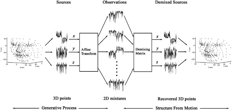
Examining the stochastic description of SfM in (3), we see that it, too, can be described as a linear mixing problem. The R matrix creates a linear mixture of s yielding the observations (mixture) w. To determine R and s in the noise-free case we seek a solution where the covariance matrix of w, denoted Σ_w, is rank 3. The relationship between the sources and observations of a general blind source separation problem and the factorization of shape and motion in structure from motion in (3) is shown in Fig. 1. As the figure shows, when a 3D object is described by a set of 3D points on the object's surface, these points can be described by an unordered sequence of 1D measurements for the x, y and z directions. In SfM, these points are assumed to undergo a transformation which includes the description of the motion and the 3D to 2D transform which generates a set of 2D observations for each frame (2D mixtures) of an image sequence of the motion. Again, the 2D observations can be described as a sequence of 1D point observations for x and y measured from the image sequence. This describes the generative process of the image sequence of observed points for an object under motion. SfM seeks to undo the generative process by recovering the transformation (demixing matrix) and the 3D shape, described by recovered 1D measurements in x, y and z, that generated the set of 1D observations. This is functionally identical to the process of recovering three 1D signals (sources) which were assumed to be mixed by a process which generates a set of 1D mixtures. Note that we will use the terms sources and shape interchangeably when describing blind source separation as it is applied to SfM. Similarly we will use the terms mixing matrix and motion matrix interchangeably.

Fig. 1.

Structure from motion as a demixing problem. A 3D face, described by points in x, y and z undergo a transformation and the demixing process recovers the transform and the original shape

A solution to the noise-free SfM problem in (3), on which Tomasi and Kanade's original factorization technique (Tomasi and Kanade 1992) is based, is provided from the Karhunen-Loeve expansion—the eigenvectors of Σ_w uniquely diagonalize it, and provide an orthonormal basis for w. In the context of SfM, the rotation matrix is thus an orthonormal basis and s corresponds to the coefficients of expansion in the basis. While the eigenvectors of Σ_w provide the only basis which diagonalize, they are not the only orthonormal basis where the resulting covariance matrix is rank 3. In fact any orthonormal transformation of the orthonormal basis of the eigenvectors is a solution as well. This implies that there is no unique solution for R and for SfM; we cannot determine the exact pose of the object, only the relative pose. Further, if s is jointly Gaussian, no further information can be extracted from the statistics of this problem, since s can be completely described by Σ_w. One solution is to exploit constraints derived from the shape (such as the existence of lines and conics, Kahl and Heyden 1999), or from photogrammetry (Zhang et al. 2003) to improve the SfM results.

In practice, however, for SfM (and for most signal processing problems), the marginal probability density functions (pdfs) of s are not Gaussian. In signal processing, this is saying that most real-world signals that contain useful information are not Gaussian. In SfM, the implication is that the distributions of points measured on a 3D object do not exhibit a Gaussian pdf in each dimension. Obviously, only a very small set of objects will have only Gaussian marginal pdfs of points relative to the set of all possible object's distributions. Given, now, that we almost always have non-Gaussian marginal pdfs for s, can we use more information to provide a solution to (3)? One obvious answer to this question is that we can use knowledge of the distribution of s. Unfortunately, we rarely have direct knowledge of the distribution of the shape points. Nonetheless, we do have knowledge that the point distributions are almost always non-Gaussian. This simple fact is sufficient to motivate our use of independent component analysis (ICA) to provide a solution to SfM problems.

Obviously, ICA cannot provide any improvement on the shape estimate over the KLT (Karhunen-Loeve Transform) in the noise-free case, since the KLT estimate is exact. Yet, ICA solutions to (3) differ from a KLT approach in one major way—they do not have a rotation ambiguity. In fact, in some ICA algorithms (FastICA, Hyvarinen et al. 2001, is a notable example), (3) is solved by first whitening x via a variance scaled KLT which reduces ICA to finding the specific rotation which will make the sources x maximally independent in the whitened space.

If noise is present in the measurement of the 2D points (as is almost always the case), a different approach is required. The direct factorization approaches described above are sensitive to noise and with the exception of the unlikely case where we have jointly Gaussian shape and noise pdfs, where shape and noise are independent, there are better approaches. We will now describe these and illustrate how ICA offers advantages in this context. A first look at modeling SFM as a BSS problem was done in Fortuna and Martinez (2006). In the present paper we will expand on this by fully developing our BSS approach, detailing the advantages that ICA offers and by providing compelling experimental evaluation.

1.2 Stochastic View of Noisy SfM

For most practical SfM problems, it is necessary to include noise in the model. Thus, we have a stochastic noisy SfM model defined as

$$\mathbf{\text{W}}=\mathbf{\text{Rs}}+\text{n},$$ (4)

where w, R and s are defined as in (3) and n is a 2F-dimensional random vector representing the noise in the observations for all frames. If we use the approach of the KLT described in the above section, we will arrive at the optimal solution for the problem defined in (4) if the distribution of s is jointly Gaussian and the noise n is also jointly Gaussian and independent of the distribution of s. For this case, we have

$${\sum }_w=\mathbf{\text{R}}E\left({\mathbf{\text{ss}}}^T\right){\mathbf{\text{R}}}^T+E\left({\mathbf{\text{nn}}}^T\right),$$ (5)

where Σ_w completely describes both the shape and the noise, since both are jointly Gaussian. Therefore, through the use of the KLT we have used all of the available information about the shape and the noise.

However, in practice, it is highly unlikely that we will have exactly this situation. In every other case, to improve on the shape estimate, we will need prior knowledge of the nature of the shape, or the noise, or both. Previous approaches have focused on applying a noise model, as defined by a maximum likelihood (ML) method (Morris and Kanade 1998), a covariance weighted SVD (Irani and Anan-dan 2002), a closest rank r approximation (Chen and Suter 2004) or matrix perturbation theory (Jia and Martinez 2010). The maximum likelihood method is an information theoretic probabilistic implementation of the “bundle adjustment” paradigm (Triggs et al. 2000) for zero-mean Gaussian noise. This idea can be further extended to a Bayesian model, when prior information about the shape or the motion is available (Kahl and Heyden 2001) or can be estimated (Forsyth et al. 1999).

Herein, we take a different approach. As above, we will show that we can exploit the non-Gaussian nature of the shape pdf by considering the problem as noisy blind source separation. Arguably, the most direct way of dealing with noise in a BSS context is to adopt a Bayesian maximum a posteriori (MAP) approach (Hyvarinen 1998). By way of the structure from motion definition in (4), we will propose a maximum a posteriori estimation approach through the direct maximization of the joint likelihood of the shape s and the transformation R. The major advantage of our approach is that the higher order statistics that are used in the description of the shape offer a way to disambiguate shape and noise and lead to a more accurate shape estimate.

We will show that the use of ICA provides an improvement in the accuracy of the reconstructed shape over other methods and can be used to determine the absolute pose. We will also show that ICA does not require the knowledge of the shape pdf to provide this improvement. In fact, this is central to the theory of blind source separation. The key point is that we can employ a MAP approach and maximize the log-likelihood and arrive at a stable local maxima despite a significant mismatch in the pdf that is used to approximate the shape pdf (Haykin 2000). This point separates a general probabilistic approach to SfM, such as Morris and Kanade (1998) and Forsyth et al. (1999), from the ICA approach described in this paper. We will also provide experimental verification and quantification of our approach by way of shape and motion estimation in a variety of real and synthetic video sequences. The recovery of the rotation ambiguity in the rigid case as well as the reduction of shape and motion error will be illustrated.

2 Previous SfM Implementations and Our Blind Source Separation Approach

In this section we will first outline previous factorization techniques for rigid SfM, followed by a discussion of our BSS approach. We will maintain a likelihood based presentation throughout this paper and derive a basic source separation algorithm for recovering the 3-dimensional shape s from 2F observations with no noise. After that, we will consider the case of noise and recall pervious maximum likelihood approaches. We then describe our solution using maximum a posteriori formulation for separating the shape and motion. Additionally, we will provide a simple example of the utility of ICA in determining the rotation ambiguity inherent in the SVD based techniques.

An advantage to our method of examining SfM from a blind source separation viewpoint is that we can readily derive previous techniques in the same context as our approach. More importantly, however, because we make no prior assumptions about the data in our model (outside of non-Gaussian source distributions), we could adjust a great many things in our formulation: noise distribution, shape prior, motion prior, etc. Further, we can view SfM from a number of approaches simultaneously—information theoretic, likelihood, maximum non-Gaussianity, direct higher-order statistics—all of which arrive at (approximately) the same theoretical solution but have differing implementations. Herein, we have chosen to outline specific ICA approaches (information theoretic and likelihood), specific noise models (Gaussian and Laplacian), a specific approach to the shape prior (Generalized Gaussian) and have chosen not to focus on a motion prior. However, our approach can be adjusted to fit additional problem constraints as required.

2.1 SVD Solution

In the noise-free case, N = 0 in (1), in practice, the motion and shape matrices can be recovered exactly (up to an arbitrary 3 × 3 linear transformation) from the SVD for a given set of measured points W for all F frames and P points by

$$\mathbf{\text{W}}={\mathbf{\text{UDV}}}^T.$$ (6)

As such, M and S can be found by the rank 3 approximation of W ∈ ℝ^2F×P—the first 3 columns of ${\mathbf{\text{UD}}}^{\frac{\text{1}}{\text{2}}}$ and 3 rows of ${\mathbf{\text{D}}}^{\frac{1}{2}}{\mathbf{\text{V}}}^{\mathit{\text{T}}}.$ As was just mentioned, this decomposition is not unique, since

$$\mathbf{\text{W}}=(\mathbf{\text{MQ}})({\text{Q}}^{-1}\mathbf{\text{S}})=\mathbf{\text{MS}},$$

where Q ∈ ℝ^3×3 is orthonormal. Each R_f in M must have an orthogonal row space, requiring the use of some constraints to find a corrective transformation matrix Q ∈ ℝ^3×3 to be applied to R_f for all frames f. This transform can be found from a least-squares fit of an over determined set of linear equations. Written concisely from Brand (2005)

$${\left(\begin{array}{l}\text{vc}({\mathbf{\text{x}}}_f,{\mathbf{\text{y}}}_f)\\ \text{vc}({\mathbf{\text{x}}}_f-{\mathbf{\text{y}}}_f,{\mathbf{\text{x}}}_f+y_f)\end{array}\right)}^T\text{vech}({\mathbf{\text{GG}}}^T)=\mathbf{0},$$

where vech(A) is a vector representation of the lower triangular elements of a symmetric matrix A and vc(x, y) = vech(xy^T + yx^T – diag(x ○ y)). Element-wise product is denoted by ○. This defines the SfM method in Tomasi and Kanade (1992). This technique has also been applied when ║N║_F is small relative to ║S║_F leading to a least-squares solution; where ║.║_F denotes the Frobenius-norm of the matrix. This approach can be further extended to deal with large values of noise, N (Chen and Suter 2004; Jia and Martinez 2010).

2.2 ICA and Semi-parametric Density Estimation

From the stochastic model for noise-free SfM in (3), we derive an ICA solution using minimum mutual information. This derivation only assumes that the pdf of the shape points is non-Gaussian. There are a number of ways to derive an algorithm in the noise free case which uses the higher order statistical properties of the sources to determine the mixing process (Hyvarinen et al. 2001). By adopting a Bayesian framework we can maintain a consistent approach between the noise free and noisy cases. This minimum mutual information approach will show that it is possible to identify sources that are mixed by a linear mixing process without assuming that they are independent. This is most easily done in an information-theoretic context described in Hyvarinen et al. (2001) and repeated here. In this way, we will make no assumption that the shapes in SfM follow any specific probabilistic model, except that they are non-Gaussian, which, as stated in the previous section, is a reasonable assumption.

By the central limit theorem (CLT), if the marginal distributions of the shape were independent and identically distributed, the mixture of 3D points w in (3) would be more Gaussian than the original shape points s. Additionally, there are forms of the CLT which relax the restrictions of independent, identically distributed random variables (Le cam 1986). So, loosely speaking, the sum of random variables is more Gaussian than the original variables. This implies that our focus in ICA need not be on exactly independent sources. Instead, we should look for sources that are more independent than their mixtures. From the CLT, these will be more non-Gaussian than their mixtures. This is important since it removes the restriction that the sources be independent for ICA to separate the sources. Indeed, if it were a requirement that the sources were exactly independent, ICA would be of limited value, since few sources in practice would be exactly independent.

Starting from our noise-free model, when the observations are made over F frames, the stochastic model is described by

$$\mathbf{\text{w}}=\mathbf{\text{Rs}},$$ (7)

where w is now a 2F-dimensional random vector of (centered) observed points and R ∈ ℝ^2F×3 is a transformation matrix over all frames, s is a three-dimensional random vector as described above.

In the noise free case, without loss of generality, we can assume a square mixing matrix, through the use of a whitening transform. To do this and to simultaneously provide whitened sources, we find a transformation V which will provide a new set of observations z, such that

$$\mathbf{\text{z}}=\mathbf{\text{Vw}},$$ (8)

where w ∈ ℝ^2F×1 is a random vector describing all observations of the 2F mixtures. This transform can be found with

$$\mathbf{\text{V}}={\mathbf{\text{D}}}^{-\frac{1}{2}}{\mathbf{\text{E}}}^T,$$

where E is a matrix whose columns are the eigenvectors of the 2F × 2F covariance matrix of w and D is a diagonal matrix of the corresponding eigen values. Note that the rank of the covariance matrix is 3, so we only need to use the first 3 eigenvectors and eigen values to completely represent w. Therefore, V ∈ ℝ^3×2F and we can now rewrite the original problem as

$$\mathbf{\text{z}}=\mathbf{\text{VRs}}=\widehat{\mathbf{\text{M}}}\mathbf{\text{s}},$$ (9)

where M̂ is a 3 × 3 orthonormal mixing matrix.

We see that ${\mathbf{\text{ED}}}^{\frac{1}{2}}\mathbf{\text{Z}}=\mathbf{\text{W}}$, where Z is the 3 × P matrix of the ensemble of whitened sources (shapes measured in x, y and z over P points) and W is the 2F × P matrix of the ensemble of observations (2F measurements of P points). For the SVD of W in (6), the sample covariance matrix of W (WW^T) is UΣV^T VΣU^T = UΣU^T thus U diagonalizes the sample covariance matrix and U is therefore the a matrix of the eigenvectors of the sample covariance matrix of w which are defined above as E for the random vector w. Therefore, E = U and Z = V^T and the sources (shape) S found by the whitening process are simply a scaled version of those found by the SVD (similarly for the motion). With whitened Gaussian data, there are no higher order statistics and the SVD is therefore equivalent to a source separation process where the sources are assumed to be Gaussian.

To begin, we recall three results from information theory. First, the mutual information I between m scalar random variables y_i, i = 1 … m is

$$I(y_1,y_2,\dots ,y_m)=\sum _{i=1}^{m}H(y_i)-H(\mathbf{\text{y}}).$$ (10)

Second, for a linear transformation y = Ax, the entropy of the transformed variable is

$$H\left(\mathbf{\text{y}}\right)=H\left(\mathbf{\text{x}}\right)+\text{log}\left|\text{det}\mathbf{\text{A}}\right|.$$ (11)

Third, entropy expressed as an expectation is

$$H\left(y\right)=-E\left[\text{log}p\right(y\left)\right].$$ (12)

Now, from (9) and using (10) and (11) we can consider the mutual information of the shape points s = M̂^Tz,

$$I(s_1,s_2,\dots ,s_m)=-\text{log}|\text{det}{\widehat{\mathbf{\text{M}}}}^{\text{T}}|-H(\mathbf{\text{z}})+\sum _{i}H(s_i),$$ (13)

where H(z) is a constant, depending only on the initial mixtures w (see (8)).

Using (12) we have the final expression for mutual information,

$$I(s_1,s_2,\dots ,s_m)=-\text{log}|\text{det}{\widehat{\mathbf{\text{M}}}}^T|-E[\sum _{\text{i}}\text{log}{p}_i({\widehat{\mathbf{\text{m}}}}_i^T\mathbf{\text{z}})],$$ (14)

where m̂i represents the ith row in the matrix M̂. We now have an expression for the mutual information of the shape points in each dimension which we can minimize. Since me are going to optimize this equation, we have ignored the constant, which will not affect the optimality solution. In deriving this, we have not used the assumption of independence. Further, we can show that minimizing mutual information is equivalent to maximizing non-Gaussianity, as measured by negentropy.

From basic information theory, negentropy J is defined from entropy as

$$J(\mathbf{\text{y}})=H({\mathbf{\text{y}}}_{\mathit{\text{gauss}}})-H(\mathbf{\text{y}}),$$ (15)

where y_gauss is a Gaussian random vector with the same co-variance matrix as y. Negentropy is zero for Gaussian random vectors and non-negative for all other cases.

From (13), using (15) we note that negentropy and the entropy of s_i only differs by the sign and an additive constant. Further, since M is orthonormal, detM̂ is a constant (equal to 1). Therefore,

$$I(s_1,s_2,\dots ,s_n)=\text{const}-\sum _{i}J(s_i).$$ (16)

So to minimize mutual information, we can maximize the sum of the non-Gaussianities of our ICA estimates, which justifies our approach to only make the assumption of non-Gaussianity when applying ICA.

The resulting solution provides an expression to maximize with respect to M̂,

$$\text{log}|\text{det}{\widehat{\mathbf{\text{M}}}}^T|+G,$$ (17)

where

$$G=E[\sum _i\text{log}{p}_i(s_i(p))].$$ (18)

Three points are in order. First, z in (14) is a whitened version of w. Therefore, the optimization is performed in the whitened space. We generate R and s from (9) by R = V^TM̂ and s = M̂^Tz. Second, this solution is identical to a solution derived from maximum likelihood, which is why we chose to maximize the negative of the mutual information (Hyvarinen et al. 2001). Third, the expectation in the third term is over the p shape points.

In order to maximize (17) we need some way to approximate the density of s_i (G in (17)). As was mentioned previously, it is not necessary to have exact knowledge of the shape pdfs to arrive at a solution for ICA. In fact, it is sufficient to know in which half-space of densities the sources lie in (sub- or super-Gaussian). This is a semi-parametric density estimation approach. Intuitively, this can be accomplished by simply measuring the kurtosis of each si during the current iteration of the maximization of (17). A kurtosis > 3 would be considered super-Gaussian while kurtosis < 3 is sub-Gaussian. A theorem provided in Hyvarinen et al. (2001) and repeated in Appendix, justifies the claim that two density approximations can optimally separate sources with unknown pdf. Herein, we will employ a generalized Gaussian density to approximate either super-Gaussian (for example, Laplacian) or sub-Gaussian (for example, mixtures of Gaussians) densities. Appendix validates the use of this parameterized density. The generalized Gaussian density for the ith unit variance source is defined by Haykin (2000)

$$h_{\alpha }(y_i)=\frac{{\alpha }_i}{2\Gamma (1/{\alpha }_i)}\text{exp}{(-\frac{|y_i|}{r})}^{{\alpha }_i},$$ (19)

where Γ is the gamma function. To utilize the generalized Gaussian density for G in (17) we need to take the log of (19) and compute the expectation over all points p. This gives

$$G=\sum _{i,p}\frac{1}{2\Gamma (1/{\alpha }_i)}|s_i(p){|}^{{\alpha }_i},$$

where α is a positive constant controlling the shape of the density. With α < 2, we are describing super-Gaussian densities. Of course, with α = 1, we get a Laplacian density. For α > 2, we have sub-Gaussian densities. Unfortunately, the intuitive approach of using kurtosis as a measure to decide whether to use sub- or super-Gaussian is not robust. Therefore, as was proposed by Lee et al. (1999a) and derived in Appendix, we can select the use of sub- or super-Gaussian densities from the sign of the result of the criterion function

$$E\{{\text{sech}}^2(s_i)\}-E\{[\text{tanh}(s_i)]s_i\}$$ (20)

over all points in s.

We will also describe two shape densities, one sub-Gaussian and one super-Gaussian, as synthetic examples which we will use as G in (17) when experimentally illustrating the effectiveness of the generalized Gaussian density as an approximation. These densities are illustrative only, but will provide analytic properties useful for the demonstration of our idea. For this, consider i sources which are distributed according to

$$h_i(y_i)=\frac{1}{2{\sigma }_i}\text{exp}(-\frac{|y_i|}{{\sigma }_i}).$$ (21)

This defines a Laplacian distribution with variance σ_i². By definition, this density is super-Gaussian. If the shape densities were known a priori and scaled to unit variance, the objective function for SfM in (17) would include the log sum of these sources, or

$$G=\sum _{i,p}|s_i(p)|,$$

where the absolute value function is evaluated for each element of s_i(p).

A second, and more flexible example of source distributions is a mixture of Gaussians. By definition, this density is sub-Gaussian. For this case, the source pdf of N mixtures is described by

$$h_i(y_i)=\sum _{n=1}^N\frac{1}{2\pi {\sigma }_n}\text{exp}(-\frac{{(y_i-{\mu }_n)}^2}{{{\sigma }_n}^2}),$$ (22)

where σ_n and μ_n are the standard deviation and mean respectively of the nth mixture. Here, the objective function to be optimized for SfM in (17) would include

$$G=\sum _{i,p,n}\text{log}{h}_i(s_i(p)).$$

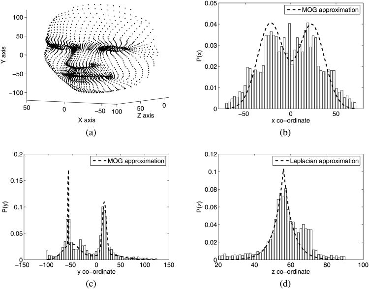
These examples are not as artificial as they might appear. For example, consider the 3D face model shown in Fig. 2(a). The distributions of the 3D points in x, y and z are shown in Figs. 2(b)–2(d), along with a Laplacian approximation of P(S_z) and mixture of Gaussian approximations of P(S_x) and P(S_y) which have been obtained with the EM algorithm (Dempster et al. 1977). Despite the complexity of the shape, simple Laplacian and mixture of Gaussians distributions provide a good density estimation.

Fig. 2.

Marginal densities of a 3D face and their Laplacian and mixture of Gaussians approximations. The 3D face model is shown in (a) and the distributions of the points P(S_x), P(S_y), P(S_z) in x, y and z are shown in (b)–(d) respectively

2.3 The Utility of ICA in Noise-free SfM

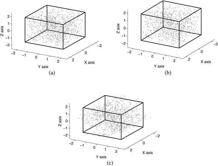
As a simple illustration of the use of ICA for recovering the motion and shape in the noise-free case, consider the following example of a shape with 100 3D points distributed uniformly inside a cube of unit variance. For this example, 25 2D images of the cube were generated, each undergoing a random 3D orthonormal transformation. Noise with a variance of 50 in both x and y was added to the 2D observations. Figure 3 shows the results obtained with ICA and the SVD, which have been rescaled to unit variance for easy view. Notice that while ICA is capable of recovering the correct shape orientation in the xy plane, the SVD solution is rotated. In this case, the original object has a non-Gaussian distribution in x, y and z and ICA provides an almost exact recovery of both the shape and its orientation in 3D space without any a priori knowledge of the object's initial orientation. This concept was first illustrated in the context of nonlinear ICA (Fujiki et al. 2004). For this example, we show that linear ICA is sufficient. It is important to note that the measure of non-Gaussianity (which provides the solution to the rotation ambiguity problem inherent in the SVD) is seen to be insensitive to the additive noise, despite the fact that, in this case, no provision was made in the ICA algorithm to model the noise. In the next section, we will further improve the shape recovery by the inclusion of a noise model.

Fig. 3.

SfM recovery of 3D points distributed uniformly inside a cube of unit variance. The distribution of the original points is shown in (a). The points recovered by ICA are shown in (b) while the recovery performed by the SVD is shown in (c)

2.4 BSS with Gaussian Noise

When we use the SfM model in (4) with a non-zero noise vector n within a source separation framework proposed in this paper, it is easy to incorporate a model of the noise or a model of both the noise and the sources in the formulation. The former results in a maximum likelihood solution and the latter represents a maximum a posteriori solution. The maximum likelihood solution was proposed previously by Morris and Kanade (1998). These two options are detailed next.

2.4.1 Maximum Likelihood Solution

If we make the assumption that the noise in (4) is Gaussian, for each frame f, the reprojection error (w_f − R_fs) can be described probabilistically by a Gaussian function and the following expression for the pdf of the observed points results

$$p({\mathbf{\text{w}}}_f|{\mathbf{\text{R}}}_f,\mathbf{\text{s}})\alpha C\text{exp}(-\frac{1}{2}{({\mathbf{\text{w}}}_f-{\mathbf{\text{R}}}_f\mathbf{\text{s}})}^T{\mathbf{\sum }}_f({\mathbf{\text{w}}}_f-{\mathbf{\text{R}}}_f\mathbf{\text{s}})),$$ (23)

where $C=\frac{1}{2\pi |{\mathbf{\sum }}_f{|}^{P/2}}$ is the normalization constant of a Gaussian distribution and Σ_f is the covariance matrix of the noise term for each frame.

Taking the log of (23), averaging over all points and frames and ignoring any scaling factors (C and number of frames and points F and P, respectively) we arrive at a maximum likelihood solution by maximizing

$$\text{log}L({\mathbf{\text{R}}}_f,\mathbf{\text{s}})=-\sum _{f=1}^F\sum _{p=1}^P\left[{║{\mathbf{\text{w}}}_f(p)-{\mathbf{\text{R}}}_f\mathbf{\text{s}}(p)║}_{{\sum }_f^{-1}}^2\right].$$ (24)

Note that the scaling can be ignored since it doesn't affect the optimality point, only its value. Equation (24) is essentially bundle adjustment (Triggs et al. 2000), with the exception that a specific Gaussian noise model is applied. Implicitly (in an information theoretic context), bundle adjustment assumes that the noise is Gaussian distributed with unit variance in x and y, although it is typically described as minimizing the 2-norm of the reprojection squared error.

A simplification that we will make in this work is that the covariance of the noise doesn't change across frames. While theoretically this is unnecessary, matters are some what complicated practically in the MAP case (detailed below) when this is not done. The issue is that if the optimization is accomplished taking each frame individually, we have F separate demixing problems where 3 sources are linearly mixed to 2 observations. This problem is under-determined. Although ICA has been shown empirically to apply in this case (Lee et al. 1999b), there are issues of the identifiability and uniqueness of the sources (Eriksson and Koivunen 2004). In short, the simplification is appropriate in practice since in most cases, the noise will occur in a similar manner for all frames.

With this argument in mind, the simplification leads to a maximum likelihood solution

$$\text{log}L(\mathbf{\text{M}},\mathbf{\text{s}})=-\sum _{p=1}^P\left[{║\mathbf{\text{w}}(p)-\mathbf{\text{Ms}}(p)║}_{{\sum }^{-1}}^2\right],$$ (25)

where w represents the random vector of 2F observations. The ML solution can be found bilinearly as described in (Morris and Kanade 1998).

The major problem associated with a ML solution is that it only takes the noise pdf into account. In fact, as mentioned previously, it is possible to use density approximations for the shape s without knowing a priori what the exact shape densities are. More importantly, a significant reduction in the error in determining the motion and shape can be obtained by the inclusion of appropriate approximations for the shape densities. This is precisely the additional advantage provided by ICA in the context of SfM. The maximum a posteriori estimation which accomplishes this, is described next.

2.4.2 MAP Solution

Maximum a posteriori estimation, as it applies to SfM can be used to maximize the joint probability of the posteriori density of the shape and the motion, that is,

$$P({\mathbf{\text{R}}}_f,\mathbf{\text{s}}|\mathbf{\text{w}})\alpha P(\mathbf{\text{w}}|{\mathbf{\text{R}}}_f,\mathbf{\text{s}})P({\mathbf{\text{R}}}_f,\mathbf{\text{s}}).$$

This defines the full a-posteriori density of both the motion and the shape. Since we are focusing on the density approximations of the shape, we will assume a uniform (uninfor-mative) prior on the motion. Under these assumptions plus the knowledge that the shape should be independent of the motion a MAP solution for M and s is given by

$$\text{arg}\underset{{\mathbf{\text{R}}}_f,\mathbf{\text{s}}}{\text{max}}P(w|{\mathbf{\text{R}}}_f,\mathbf{\text{s}})P(\mathbf{\text{s}}).$$

The log of this MAP estimate provides an objective function to maximize,

$$\text{log}L({\mathbf{\text{R}}}_f,\mathbf{\text{s}})=-\sum _{f=1}^F\sum _{p=1}^P[{║{\mathbf{\text{w}}}_f\left(p\right)-{\mathbf{\text{R}}}_f\mathbf{\text{s}}\left(p\right)║}_{{\sum }^{-1}}^2+\sum _{i=1}^3{g}_i(s_i(p))],$$ (26)

where g_i (·) = −log P_i (·) are the individual densities of unit variance sources. For this optimization, we will employ the same generalized Gaussian as for the non-noisy case described by (19) and the same criterion, described by (20) for selecting the shape of the densities and a constant co-variance matrix for the noise, giving the following objective function,

$$\text{log}L(\mathbf{\text{M}},\mathbf{\text{s}})=-\sum _{p=1}^P[{║\mathbf{\text{w}}\left(p\right)-\mathbf{\text{Ms}}\left(p\right)║}_{{\sum }^{-1}}^2+\sum _{i=1}^3{g}_i(s_i(p))].$$ (27)

Recall that in BSS, it is only necessary to determine whether the sources are sub- or super-Gaussian and this can be reliably accomplished with the current estimate of the sources. Hence, blind source separation provides the ability to recover motion and shape matrices without any knowledge of the motion or shape. Further, a model of both the noise and the shape densities can be readily included in the MAP methodology for performing ICA in the presence of noise.

A number of techniques exist to maximize the objective function in (26). Some iterative techniques resulting from direct differentiation can be found in Hyvarinen (1998), provided that the source distribution approximation is differentiable. These approaches utilize an alternating variables method. We applied general non-linear optimizers directly and found that the total optimization time was reasonable for on the order of a hundred or so points and, in any case, would be similar to that of bundle adjustment.

To summarize, when there is no noise in the point measurements, the SVD (6) can be used to exactly determine the motion matrix M and the shape matrix S up to a rotation. Additionally, (17) can be used to determine the rotation ambiguity. When the point measurements are noisy, maximum likelihood estimation uses a noise model to provide a solution by maximizing (25). If a model of both the noise and the shape are included, ICA can be employed by maximizing (27). The ICA solution represents maximum a posteriori estimation. To maximize (27) it is necessary to use the appropriate generalized Gaussian density model (sub- or super-Gaussian) for each of the sources (the shapes in x, y and z). This is accomplished by using the criterion in (20). This selection is employed at each step of a general nonlinear optimization process.

2.5 The Orthogonality Constraint on M

An additional constraint exists in SfM on the motion matrix when we use the weak-perspective model—each R_f in M has an orthonormal row space. This constraint can be applied in a couple of ways. First, the orthonormality can be enforced at each step in an iterative algorithm. Second, it can be enforced after the computation of M. If the latter method is used, the rows are only approximately orthonormal, as determined by a least-squares solution (Tomasi and Kanade 1992). A significant improvement to the ML algorithm described in Morris and Kanade (1998) can be achieved by orthonormalizing the motion matrix at each step in the algorithm. Alternatively, the motion matrix can be described by quaternians, which parameterizes a rotation matrix so that the result is orthonormal in the parameter space. We use this technique in all of the optimizations (bundle adjustment, maximum likelihood and maximum a posteriori) presented in the section to follow. Note that for when there is no noise a closed form solution exists (Tomasi and Kanade 1992), which finds a transformation of M to enforce the constraint of orthonormality. However, in the noisy case, no such solution exists, due to its uncertainty.

3 Experimental Results

The previous section provided the details of the two claims that we make in this paper:

1. Rigid SfM can be described as a blind source separation problem. Implicit in this claim is the idea that it is not necessary to have complete knowledge of the source pdfs to employ MAP estimation for SfM.

2. Our formulation will provide an improvement to the quality of the shape estimate via the use of the non-Gaussianity of the sources irrespective of the shape pdf.

To evaluate the BSS formulation derived in this paper, we present a set of experimental results with synthetic and real data. We start with a large variety of synthetic examples in the first experimental section below. These examples are provided to validate the use of blind source separation techniques by comparing MAP with and without explicit knowledge of the source pdfs. The second experimental section illustrates the improvement obtained from the use of our approach on the reconstruction of 3D shapes from noisy tracked fiducials.

3.1 Statistical Comparison of SVD, ML and MAP

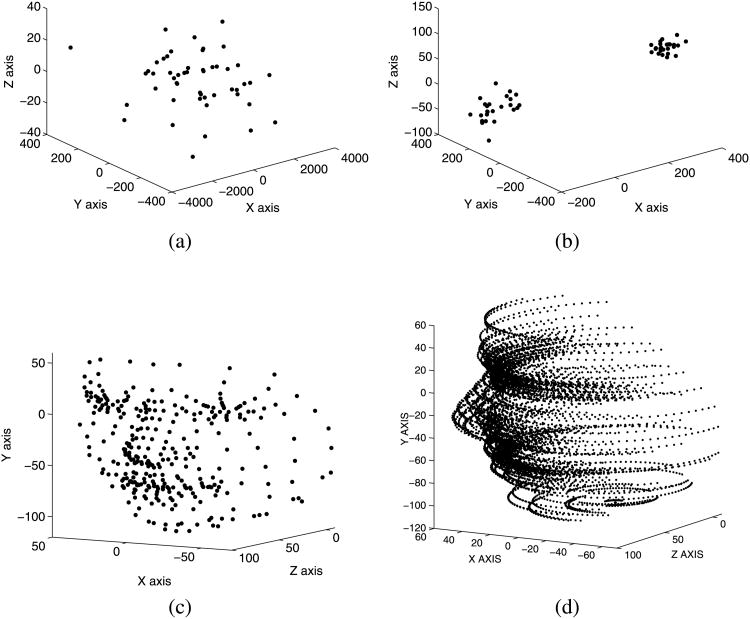
We start with three synthetic examples generated with 50 points according to Laplacian densities, mixtures of Gaussian densities and a face model, respectively. Specifically, the two distributions described in (21) and (22) were used to generate statistically independent 3D sources. In the Laplacian case, the source variances were 1,000, 100, and 10 for the x, y and z directions. For the mixture of Gaussian sources, two mixtures for each direction were considered. The x direction had means of −100 and 300 with variances 2,000 and 1,000. The y direction had means of 200 and −200 with variances 200 and 100. The z direction had means of −30 and 90 with variance of 100 in both cases. Figures 4(a) and 4(b) provide samples of the point distributions. Figure 4(c) shows the 3D face model consisting of approximately 350 points, from which 50 points were selected at random for our experiment. For the Laplacian and mixture of Gaussians densities, a random transformation matrix was generated for each frame. For the face model, a rotation of 90 degrees about the y axis was generated as a geometric transformation, Fig. 4(d). Gaussian noise was then added to the 2D point data resulting from the projection of the 3D points. The resulting 2D points were then centered for the x and y directions. A similar methodology was applied to generate 2D points from a 3D reconstruction of the dinosaur data sequence (Buchanan and Fitzgibbon 2005) using 319 3D points which were considered “inliers”.

Fig. 4.

3D points—(a) Laplacian distributed, (b) Mixture of Gaussian Distributed, (c) Face model, (d) Face model rotated about the y axis

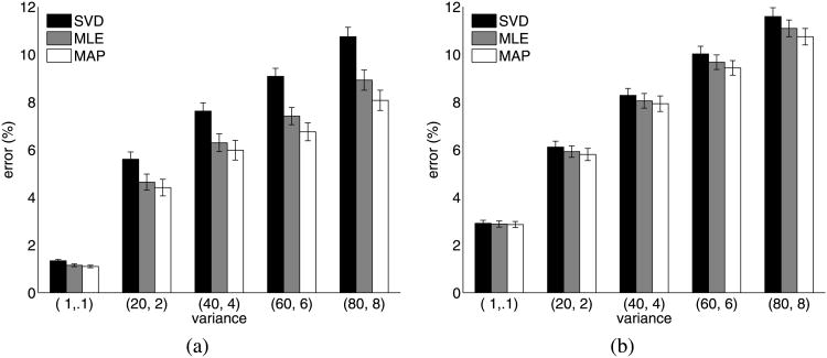
For the Laplacian and mixture of Gaussian points, the noise variance was parameterized to 1, 100, 200, 300 and 400 for the x direction and .1, 10, 20, 30 and 40 for the y direction, creating 5 independent experiments for each of the two source distributions. For the face data, the noise variance was parameterized to 1, 20, 40, 60 and 80 for the x direction and .1, 2, 4, 6 and 8 for the y direction. The motion and the structure matrix were recovered for each experiment with 3 different techniques—SVD, ML estimation, and MAP estimation. All estimates were referenced to the co-ordinate system of the first frame of the ground-truth.

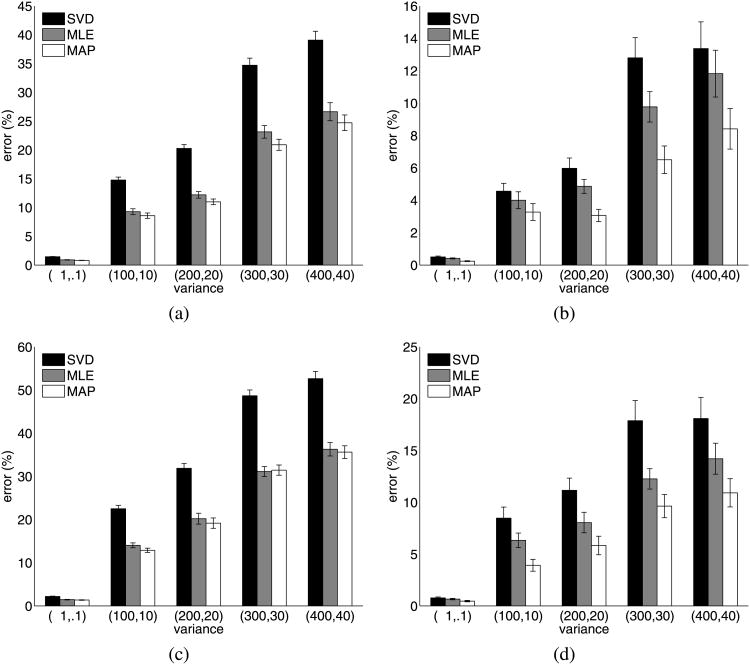
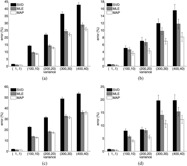
In Tables 1 and 2, the first two priors (Laplacian and mixture of Gaussians) illustrate the use of MAP estimation when the source distributions are known a priori and are applied directly to the cost function. Figure 5 describes the mean motion and shape errors. Tables 3 and 4 illustrate the main idea of the work presented in this paper—the results of recovering the motion and shape matrices of a Laplacian shape density with a super-Gaussian prior and a mixture of Gaussian shape density with a sub-Gaussian prior. The priors were a generalized Gaussian density where (20) was employed during the optimization to determine which form of density to employ. Specifically, α in (19) can be switched between 1 and 3, corresponding to super and sub-Gaussian densities, respectively. Figure 7 describes the mean errors in the recovered motion and shape matrices over 50 runs. The mean errors are reported as the norm of the error in the estimated matrix expressed as a percentage of the norm of the ground-truth matrix. Since these errors were decidedly non-Gaussian in distribution, we have also provided box-plots (Figs. 6(a)–6(b)) of the largest measured estimation errors with our technique.

Table 1. Errors in motion and shape matrices—Laplacian distributed shapes.

Noise Σ		$\left(\begin{array}{cc}1& 0\\ 0& 0.1\end{array}\right)$		$\left(\begin{array}{cc}100& 0\\ 0& 10\end{array}\right)$		$\left(\begin{array}{cc}200& 0\\ 0& 20\end{array}\right)$		$\left(\begin{array}{cc}300& 0\\ 0& 30\end{array}\right)$		$\left(\begin{array}{cc}400& 0\\ 0& 40\end{array}\right)$
		μ	σ2	μ	σ2	μ	σ2	μ	σ2	μ	σ2
Error (motion)	SVD	1.44	0.13	14.77	12.61	20.25	22.93	34.71	74.77	39.07	118.80
	ML	0.90	0.07	9.26	12.93	12.19	16.71	23.13	59.12	26.63	122.94
	MAP	0.80	0.05	8.57	11.02	10.98	12.05	20.89	46.53	24.71	92.88
Error (shape)	SVD	0.50	0.14	4.56	11.79	5.97	20.56	12.80	77.34	13.37	135.77
	ML	0.41	0.05	4.00	13.67	4.86	9.24	9.77	44.40	11.82	104.43
	MAP	0.24	0.04	3.27	13.67	3.06	7.18	6.50	36.36	8.41	78.43

Table 2. Errors in motion and shape matrices—Mixture of Gaussian distributed shapes.

Noise Σ		$\left(\begin{array}{cc}1& 0\\ 0& 0.1\end{array}\right)$		$\left(\begin{array}{cc}100& 0\\ 0& 10\end{array}\right)$		$\left(\begin{array}{cc}200& 0\\ 0& 20\end{array}\right)$		$\left(\begin{array}{cc}300& 0\\ 0& 30\end{array}\right)$		$\left(\begin{array}{cc}400& 0\\ 0& 40\end{array}\right)$
		μ	σ2	μ	σ2	μ	σ2	μ	σ2	μ	σ2
Error (motion)	SVD	2.18	0.34	22.50	32.17	31.88	62.63	48.67	89.72	52.63	138.20
	ML	1.45	0.30	14.03	15.65	20.20	79.93	31.12	66.47	36.28	123.22
	MAP	1.36	0.26	12.88	12.30	19.16	72.82	31.44	70.40	35.61	109.32
Error (shape)	SVD	0.77	0.39	8.47	56.53	11.15	69.73	17.87	188.97	18.08	207.09
	ML	0.66	0.25	6.33	24.46	8.04	49.23	12.26	48.24	14.20	111.37
	MAP	0.46	0.24	3.92	16.40	5.83	40.23	9.63	62.60	10.91	93.01

Fig. 5.

Results showing (a) motion error for a Laplacian distributed shape with a Laplacian pdf model, (b) shape error for a Laplacian distributed shape with a Laplacian pdf model, (c) motion error for a mixture of Gaussian distributed shape with a mixture of Gaussian pdf model (d) shape error for a mixture of Gaussian distributed shape with a mixture of Gaussian pdf model. Note that, thanks to the addition of the shape prior, the errors in (b) and (d) are much smaller than those in (a) and (c)

Table 3. Errors in motion and shape matrices—super-Gaussian distributed shapes.

Noise Σ		$\left(\begin{array}{cc}1& 0\\ 0& 0.1\end{array}\right)$		$\left(\begin{array}{cc}100& 0\\ 0& 10\end{array}\right)$		$\left(\begin{array}{cc}200& 0\\ 0& 20\end{array}\right)$		$\left(\begin{array}{cc}300& 0\\ 0& 30\end{array}\right)$		$\left(\begin{array}{cc}400& 0\\ 0& 40\end{array}\right)$
		μ	σ2	μ	σ2	μ	σ2	μ	σ2	μ	σ2
Error (motion)	SVD	1.47	0.18	14.17	13.23	21.89	49.04	36.35	113.57	42.68	114.40
	ML	0.92	0.14	9.51	12.83	14.25	33.26	24.26	70.68	28.80	96.78
	MAP	0.82	0.11	8.57	11.71	12.74	19.78	22.06	55.81	25.79	71.93
Error (shape)	SVD	0.51	0.19	5.05	19.89	7.03	48.81	11.94	74.20	15.53	142.99
	ML	0.44	0.12	4.62	12.95	6.65	33.91	9.77	44.92	11.77	86.54
	MAP	0.28	0.09	3.60	14.21	4.26	22.75	6.97	32.85	8.14	76.03

Table 4. Errors in motion and shape matrices—sub-Gaussian distributed shapes.

Noise Σ		$\left(\begin{array}{cc}1& 0\\ 0& 0.1\end{array}\right)$		$\left(\begin{array}{cc}100& 0\\ 0& 10\end{array}\right)$		$\left(\begin{array}{cc}200& 0\\ 0& 20\end{array}\right)$		$\left(\begin{array}{cc}300& 0\\ 0& 30\end{array}\right)$		$\left(\begin{array}{cc}400& 0\\ 0& 40\end{array}\right)$
		μ	σ2	μ	σ2	μ	σ2	μ	σ2	μ	σ2
Error (motion)	SVD	2.03	0.34	22.50	29.88	31.35	51.90	48.75	108.07	53.45	97.37
	ML	1.34	0.22	13.62	16.17	18.16	22.00	32.60	95.84	36.25	115.40
	MAP	1.24	0.15	12.67	11.83	17.24	20.91	31.26	65.50	35.77	93.34
Error (shape)	SVD	0.81	0.56	7.91	27.73	8.40	38.15	19.60	217.93	19.68	236.57
	ML	0.61	0.32	5.65	12.53	8.05	34.85	13.99	126.50	15.33	132.54
	MAP	0.43	0.23	4.01	9.33	5.50	27.98	10.62	95.62	12.28	117.49

Fig. 7.

Results showing (a) motion error for Laplacian distributed shape with a generalized Gaussian pdf model, (b) shape error for Laplacian distributed shape with a generalized Gaussian pdf model, (c) motion error for mixture of Gaussian distributed shape with a generalized Gaussian pdf model, (d) shape error for mixture of Gaussian distributed shape with a generalized pdf model

Fig. 6. Boxplots of the synthetic shape errors. (a) Super-Gaussian (b) Sub-Gaussian (c) Faces.

Table 5 provides the mean motion and shape estimation error over 50 runs of the randomly selected 50 face model points. Figure 6(c) provides a boxplot of the results with the largest measured shape estimation errors. Table 6 provides the mean motion, shape and reprojection estimation error over 50 runs of all 319 points of the reconstruction of the dinosaur sequence Here, as in the Laplacian and mixture of Gaussian points, (20) was used to determine the prior during optimization.

Table 5. Errors in motion and shape matrices—face model data.

Noise Σ		$\left(\begin{array}{cc}1& 0\\ 0& 0.1\end{array}\right)$		$\left(\begin{array}{cc}20& 0\\ 0& 2\end{array}\right)$		$\left(\begin{array}{cc}40& 0\\ 0& 4\end{array}\right)$		$\left(\begin{array}{cc}60& 0\\ 0& 6\end{array}\right)$		$\left(\begin{array}{cc}80& 0\\ 0& 8\end{array}\right)$
		μ	σ2	μ	σ2	μ	σ2	μ	σ2	μ	σ2
Error (motion)	SVD	1.34	0.13	5.60	4.70	7.62	5.83	9.08	5.58	10.74	7.85
	ML	1.15	0.17	4.64	5.66	6.29	6.88	7.41	6.51	8.92	8.96
	MAP	1.10	0.15	4.41	6.12	5.98	8.45	6.75	7.05	8.07	9.06
Error (shape)	SVD	2.91	0.82	6.11	3.06	8.28	4.23	10.02	5.14	11.59	6.67
	ML	2.88	0.85	5.92	2.92	8.05	4.71	9.67	4.65	11.09	6.16
	MAP	2.86	0.84	5.80	3.24	7.93	5.36	9.43	4.70	10.74	6.03

Table 6. Errors in motion, shape and reprojection matrices—dinosaur sequence data.

Noise Σ		$\left(\begin{array}{cc}1& 0\\ 0& 0.1\end{array}\right)$		$\left(\begin{array}{cc}1E4& 0\\ 0& 1E3\end{array}\right)$		$\left(\begin{array}{cc}2E4& 0\\ 0& 2E3\end{array}\right)$		$\left(\begin{array}{cc}3E4& 0\\ 0& 3E3\end{array}\right)$		$\left(\begin{array}{cc}4E4& 0\\ 0& 4E3\end{array}\right)$
		μ	σ2	μ	σ2	μ	σ2	μ	σ2	μ	σ2
Error (motion)	SVD	0.02	0.00	2.18	0.16	3.26	0.41	4.32	0.78	5.18	1.22
	ML	0.02	0.00	1.53	0.07	2.24	0.14	2.71	0.22	3.15	0.31
	MAP	0.02	0.00	1.26	0.08	1.81	0.15	2.13	0.30	2.47	0.42
Error (shape)	SVD	0.06	0.00	6.33	0.13	9.28	0.47	11.83	1.19	14.09	2.11
	ML	0.05	0.00	5.34	0.05	7.63	0.12	9.43	0.23	10.93	0.35
	MAP	0.05	0.00	5.34	0.05	7.63	0.12	9.43	0.23	10.93	0.35
Error (reproj.)	SVD	0.04	0.00	3.76	0.01	5.38	0.01	6.61	0.03	7.69	0.05
	ML	0.03	0.00	3.33	0.01	4.76	0.02	5.81	0.04	6.73	0.05
	MAP	0.03	0.00	3.23	0.01	4.62	0.01	5.63	0.03	6.54	0.04

As expected, in all of the previous experiments, the error in both motion and shape increase with increased noise variance. The key point that these experiments illustrate is that when Tables 1 and 3 are compared, there is little difference between the means of the errors in the estimated motion or shape for all levels of noise variance. Recall that the first table describes the result when the Laplacian shape pdf is known a priori and the second describes the results when using blind source separation with a generalized Gaussian. For example, at the largest value of noise variance, the shape error with a known pdf is 8.41 percent, while it is 8.14 percent when no knowledge of the shape pdf is used a priori. A similar result is illustrated by comparing Tables 2 and 4, obtained by using a mixture of Gaussian pdf model a priori and the generalized Gaussian with BSS, respectively. In that case, for example, at the largest value of noise variance, the shape error with a known pdf is 10.91 percent, while it is 12.28 percent when no knowledge of the shape pdf is used a priori. These results clearly validate our first claim that it is not necessary to know the shape pdf a priori to employ MAP estimation and thus experimentally justify the use of blind source separation techniques.

In examining Fig. 5 we note that there is a statistically significant (p ≤ 0.05) difference between the shape reconstruction quality over MLE with the use of MAP estimation when the pdf of the sources is known a priori, provided that the noise variance is large enough (greater than 100 in x and 10 in y). We would, of course, expect that for smaller values of noise variance, the advantage of MAP estimation would be reduced. This result illustrates that knowledge of the shape pdf can be used to improve the quality of the reconstruction, which is to be expected. Also as expected, the motion estimate does not improve significantly from a maximum likelihood formulation.

More interesting, in Fig. 7 we illustrate the second claim of this paper—a statistically significant improvement in the shape reconstruction can be made with MAP estimation without explicit knowledge of the shape pdf. All that is necessary is to estimate whether the shape distribution is super-or sub-Gaussian. Again, for all values of noise variance greater than 100 in x and 10 in y, we observe a statistically significant (p ≤ 0.05) difference between the shape reconstruction quality of MLE with the use of MAP estimation when the pdf of the sources is not known a priori.

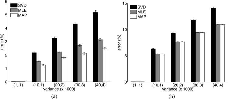
In Fig. 8, we show the mean errors in motion and shape estimation for a synthetic face model. We see that a statistically significant improvement in the motion estimate is obtained for variance greater than 60 in x and 6 in y, and the shape estimate improvement of MAP over MLE misses significance. Further, in Fig. 9, a similar result to the face model is seen. All of the motion estimates for the MAP approach are statistically significantly better than the MLE or SVD approaches. It should be noted, also, that in order to align the shapes for measurement with respect to the ground truth, the shape estimate error is minimized in a least-squares sense. As a result, it is possible that although we optimize for minimum shape error, after we align the estimate and ground truth, it may be that the improvement is seen in the motion estimate. In any case, on the whole, these experiments provide a convincing argument that blind source separation techniques will improve the shape estimate over MLE, irrespective of the shape pdf.

Fig. 8. Results—(a) Face with generalized pdf model-motion, (b) Face with generalized pdf model-shape.

Fig. 9. Results—(a) Dinosaur sequence with generalized pdf model-motion, (b) Dinosaur sequence with generalized pdf model-shape.

3.2 Reconstruction of Real Data from Noisy Tracked Fiducials

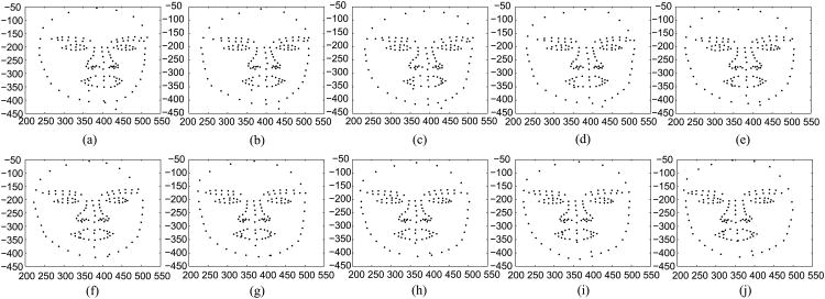
In our final study, we consider the reconstruction of two commonly used datasets and a third dataset that we collected from a video of tracked facial fiducials. The common datasets included a publicly available origami cube sequence www-cvr.ai.uiuc.edu/ponce_grp/data/zeroskew/data.tgz, the Model House Sequence (Fitzgibbon and Zisserman 1998) and the previously used dinosaur sequence. In all cases, we selected points which were visible over a minimum of 5 frames which gave us 175 points over 5 frames for the cube data, 275 points over 15 frames for the house data, 139 points over 17 frames for the face data and 319 points over 21 frames for the dinosaur sequence. The tracked face points correspond to a video sequence of a real face filmed as it moves in 3D with minimal change in expression. Figure 10 shows the frames of the 139 tracked points from the face video sequence. The facial detection of these points was obtained using the algorithm described in Ding and Martinez (2008).

Fig. 10. Tracked face points for 10 video frames.

For these examples, two experiments were conducted with 50 runs of randomly generated noise. The first experiment used Gaussian noise added to the 2D tracked points with a variance of 50, 50, 10 and 10,000 in both the x and y reprojected directions for the cube, house, face and dinosaur data respectively. The second study used outliers generated as a uniform distribution with a width of 20, 20, 5 and 500 in x and y applied to 30% of the points (selected at random) for the cube, house, face and dinosaur data respectively. Both the outliers and Gaussian noise experiments were reconstructed with 3 different techniques—SVD, ML, and our MAP approach.

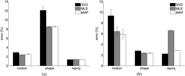
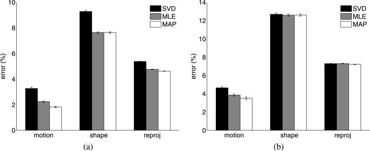
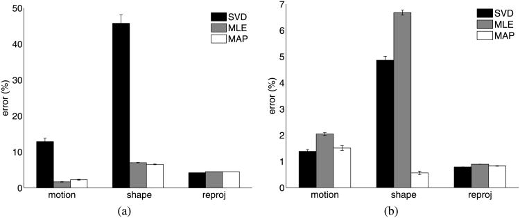
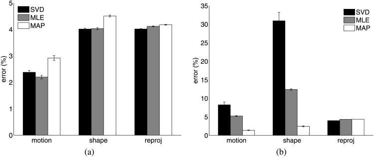
Tables 7 and 8 illustrate the application of MAP estimation to real data with Gaussian noise and outliers, respectively. Note that here we don't have a ground-truth to measure the results against. As a result, we are describing the sensitivity of the 3D measurement to noise and also indicate the reprojection error. From Table 7 we see that the shape error provided by the MAP estimation was equal to or better than the next best approach. The real data results are summarized in Figs. 11–14. While the MAP shape estimate was not always statistically significantly better than MLE, it was statistically significantly equal to or better than MLE in all but the house data with outliers.

Table 7. Errors in motion and shape matrices with Gaussian Noise—tracked fiducial data.

Error		Motion		Shape		Reprojection
		μ	σ2	μ	σ2	μ	σ2
Cube Data	SVD	2.89	2.16	12.08	30.67	1.35	0.0014
	ML	2.39	0.23	8.51	0.70	1.40	0.0012
	MAP	2.54	0.30	8.51	0.70	1.34	0.0015
House Data	SVD	9.34	66.51	2.78	1.70	2.23	0.0004
	ML	6.42	35.54	2.39	0.83	6.58	0.74
	MAP	5.89	37.35	2.37	0.85	2.87	0.0079
Face Data	SVD	12.85	45.27	45.74	279.53	4.19	0.0002
	ML	1.66	0.28	7.01	0.30	4.49	0.0005
	MAP	2.26	0.63	6.54	0.35	4.49	0.0005
Dinosaur Data	SVD	3.26	0.41	9.29	0.47	5.38	0.01
	ML	2.24	0.14	7.63	0.12	4.76	0.02
	MAP	1.81	0.15	7.63	0.12	4.62	0.01

Table 8. Errors in motion and shape matrices with outliers—tracked fiducial data.

Error		Motion		Shape		Reprojection
		μ	σ2	μ	σ2	μ	σ2
Cube Data	SVD	1.38	0.20	4.86	1.07	0.79	0.0004
	ML	2.05	0.13	6.67	0.46	0.90	0.0003
	MAP	1.51	0.45	0.56	0.22	0.82	0.0028
House Data	SVD	2.38	0.25	4.01	0.06	4.01	0.0067
	ML	2.20	0.24	4.03	0.06	4.11	0.0086
	MAP	2.92	0.42	4.51	0.07	4.18	0.0089
Face Data	SVD	8.25	27.44	30.93	262.69	3.98	0
	ML	5.22	0.64	12.38	2.34	4.31	0.0001
	MAP	1.37	0.32	2.44	0.80	4.35	0.0003
Dinosaur Data	SVD	4.64	0.90	12.69	0.84	7.29	0.03
	ML	3.85	0.79	12.59	0.67	7.29	0.04
	MAP	3.50	1.10	12.59	0.67	7.21	0.04

Fig. 11. Results: (a) Cube Data—Gaussian noise, (b) Cube Data—outliers.

Fig. 14. Results: (a) Dinosaur Sequence—Gaussian noise, (b) Dinosaur Sequence—outliers.

It is important to note that all of these sensitivity results were obtained using a starting point derived from the noise-free solution for each technique. All of these techniques are optimization techniques and only the SVD has a global solution, therefore they are sensitive to the initialization point. In practice, this ideal starting point cannot usually be obtained. None the less, we are evaluating the sensitivity of the approach to noise, which is the best that we can do in the absence of ground truth data. As a final note on the optimization techniques employed in this work, all were performed with Matlab's unconstrained non-linear optimization routine—fminunc. For the largest data set (319 points and 21 frames), we performed one iteration in approximately 2 seconds. In no cases did our routines converge in more than 500 iterations. Most were under 100 iterations. This gives a worst case computation time of about 17 minutes (Intel Core 2 Duo CPU, 1.60 GHz, 3 GB ram). Most took under 4 minutes. Note that this is considerably longer than the MLE approach, which typically converges in under a minute. It is thus fair to say that our implementation took an order of magnitude longer to converge than MLE. To improve upon this result, one could employ a faster noisy ICA algorithms (Cichocki et al. 1998). In the present paper, we simply selected an implementation that directly followed our objective functions for the purpose of clarity.

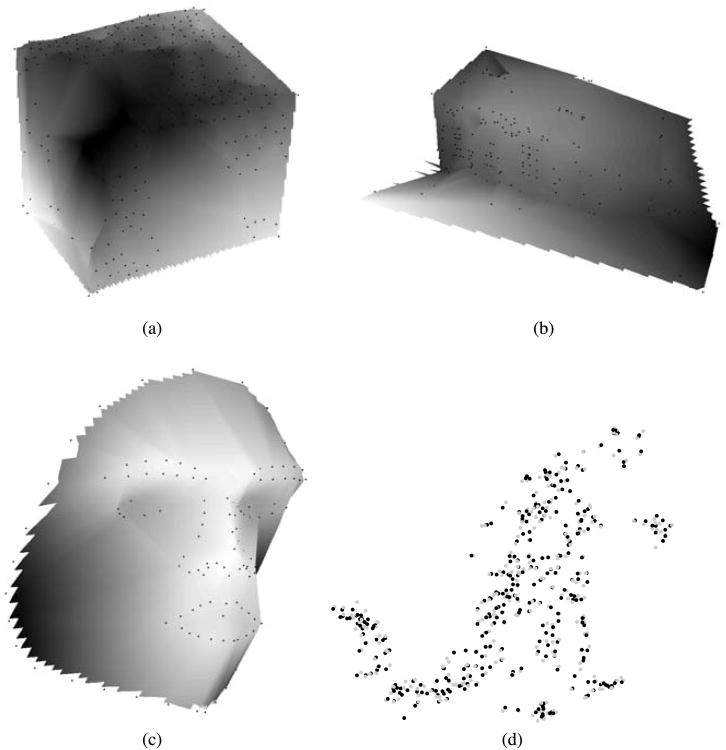
Finally, we show the 3D reconstruction provided by MAP estimation to the tracked points data in Fig. 15. In the first three of these reconstructions, we do not add any synthetic noise to the data points since these are real tracked points. In the last reconstruction (the dinosaur) we added Gaussian noise with a variance of 10,000 in both x and y. The original reconstruction is shown with black points and the noisy reconstruction using MAP is shown with gray points. Note that the difference in reconstruction error of all of these figures between the SVD, MLE and MAP is less than 1 percent. This cannot be easily visualized. As a result, we have only shown the MAP reconstruction for illustrative purposes only—the error tables and plots provide a complete quantitative description.

Fig. 15. MAP shape reconstructions (a) Cube (b) House (c) Face (d) Dinosaur.

4 Conclusion

We have shown that a significant improvement in shape estimate can be obtained from a MAP approach to structure from motion. More importantly, explicit knowledge of the shape pdf is not needed to obtain this improvement. In fact, the theory of blind source separation, for which we have shown that SfM applies directly, dictates that we can optimally reconstruct the shape and motion without explicit knowledge of the shape pdf. In a sense, we can use the non-Gaussianity of the shape pdf in each direction to provide an improvement over maximum likelihood without prior knowledge. Since the vast majority of real-world shape pdfs are non-Gaussian, our approach is as applicable as maximum likelihood and, by extension of it, bundle adjustment. We have validated the use of our blind source separation framework through extensive experimental data. As the theory of blind source separation in the presence of noise advances, so too will its application to structure from motion. The SfM approach derived in this paper should provide an indication of where such improvements should be directed.

Fig. 12. Results: (a) House Data—Gaussian noise, (b) House Data—outliers.

Fig. 13. Results: (a) Tracked Face Points—Gaussian noise, (b) Tracked Face Points—outliers.

Appendix

Theorem 1 If the input data follows the model in (9) and we employ a smooth even function G, the local maxima of the expectation of G(m̂^Tz) with ║m̂║ = 1 will be satisfied by the rows of the mixing matrix M̂ so that the corresponding s_i satisfy

$$E\{s_{i}g(s_i)-g^{\text{'}}(s_i)\}>0,$$ (A.1)

where g(.) is the derivative of g(.), g′(·) is the derivative of g(.), m̂_i denotes the ith row of M̂ and s_i denotes the ith source.

This theorem states that if we consider a whitened representation of the sources and we apply any non-linearity G to approximate the actual density, we will arrive at the same local maxima as long as the condition in (A.1) is satisfied.

The remaining question is which function is most appropriate for G. In fact, a sufficiently close approximation to the actual source densities where Theorem 1 holds is all that is necessary. So as long as we use densities that satisfy (A.1), we will still arrive at the optimal local maximum of the likelihood. As an example of 2 simple functions which satisfy the theorem, consider

$$g^{+}(s_i)=-2\text{tanh}(s_i)$$ (A.2)

and

$$g^{-}(s_i)=\text{tanh}(s_i)-s_i.$$ (A.3)

From (A.1), using the fact that the derivative of tanh (s) = 1 − tanh²(s), we arrive at a criterion for the selection of the functions g⁺ and g⁻, by always making the sign of the expectation in (A.1) positive. For g⁺ we have E{−s_i tanh(s_i) + (1 − tanh² (s_i))} and for g⁻ we have E{s_i tanh(s_i) – (1 – tanh²(s_i))}. Further, 1 − tanh²(s) = sech²(s) and we can write a criterion which, based on the sign of the result, will provide the function which satisfies the inequality in the theorem, i.e.,

$$E\{{\text{sech}}^2(s_i)-s_i\text{tanh}(s_i)\}>0$$ (A.4)

for the g⁺ and

$$E\{{\text{sech}}^2(s_i)-s_i\text{tanh}(s_i)\}<0$$ (A.5)

for g⁻. This is precisely the criterion derived by Lee et al. (1999a) and the one that we use in this paper.

We are using the generalized Gaussian density function in our optimization function, since we are comparing the results to specifically chosen sub- and super-Gaussian densities. This density for i unit variance sources is defined by Haykin (2000)

$$h_{\alpha }(y_i)=\frac{{\alpha }_i}{2\Gamma (1/{\alpha }_i)}\text{exp}{(-\frac{|y_i|}{r})}^{{\alpha }_i},$$ (A.6)

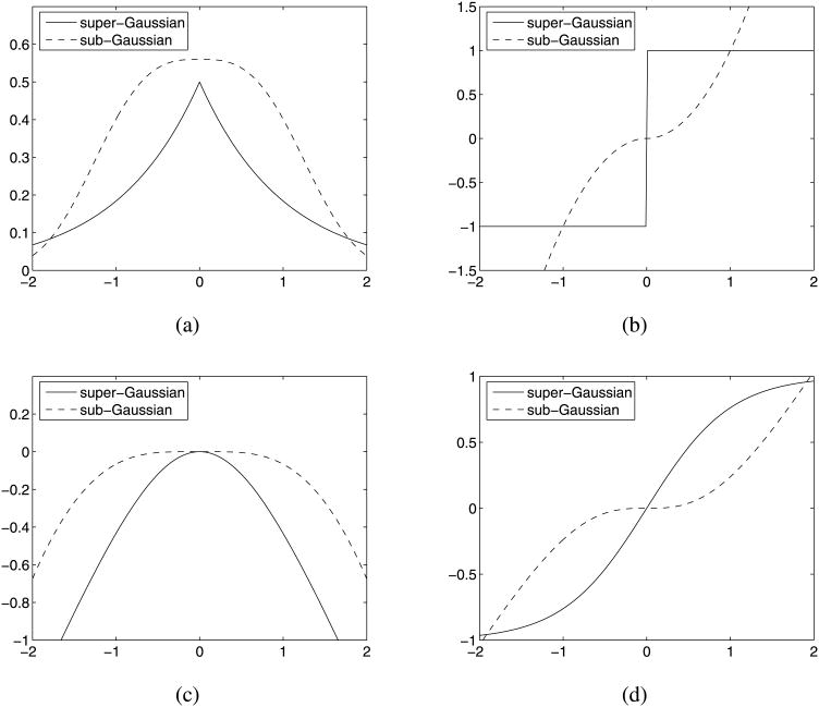
where Γ is the gamma function and r defines the measure of spread. The generalized Gaussian that we employ has derivatives that closely approximate g⁺ and g⁻ depending on the selection of the exponent of the Gaussian. The generalized Gaussian has the advantage of exactly approximating the super-Gaussian density which we use in our examples. This is not true of the pdf corresponding to g⁺ used in the derivation. Unfortunately, for the purposes of the theorem, we had to use a function whose the 2nd derivative was everywhere differentiable. The generalized Gaussian does not satisfy this property. So we instead used a tanh based approximation for g in theorem and we now show visually that the generalized Gaussian closely approximates the tanh based approximation. Figure 16 shows the pdf and derivative functions g for both the generalized Gaussian pdf defined in (A.6) and the tanh derivative function.

Fig. 16.

Generalized Gaussian and tanh density approximations. The generalized Gaussian pdf and its derivative g are shown in (a) and (b) respectively. The tanh derivative's corresponding pdf and the tanh function used for g are shown (c) and (d) respectively

References

- Belouchrani A, Abed-Meraim K, Cardoso JF, Moulines E. A blind source separation technique using second-order statistics. IEEE Transactions on Signal Processing. 1997;45(2):434–444. [Google Scholar]
- Brand M. A direct method for 3D factorization of nonrigid motion observed in 2D. Proc. IEEE conference on computer vision and pattern recognition; San Diego (CA). Los Alamitos: IEEE Comput. Soc; 2005. pp. 122–128. [Google Scholar]
- Buchanan AM, Fitzgibbon AW. Proc IEEE computer society conference on computer vision and pattern recognition. Vol. 2. Los Alamitos: IEEE Comput. Soc; 2005. Damped Newton algorithms for matrix factorization with missing data; pp. 316–322. [Google Scholar]
- Chen P, Suter D. Recovering the missing components in a large noisy low-rank matrix: application to SFM. IEEE Transactions on Pattern Analysis and Machine Intelligence. 2004;26(8):1051–1063. doi: 10.1109/TPAMI.2004.52. [DOI] [PubMed] [Google Scholar]
- Cichocki A, Douglas S, Amari S. Robust techniques for independent component analysis (ICA) with noisy data. Neurocomputing. 1998;22:113–129. [Google Scholar]
- Dempster AP, Laird NM, Rubin DB. Maximum likelihood from incomplete data via the EM algorithm. Journal Royal Statistical Society. 1977;30(1):1–38. [Google Scholar]
- Ding L, Martinez AM. Precise detailed detection of faces and facial features. Proc. IEEE conference on computer vision and patter recognition; Anchorage (AK). Los Alamitos: IEEE Comput. Soc; 2008. [Google Scholar]
- Eriksson J, Koivunen V. Identifiability, separability, and uniqueness of linear ICA models. IEEE Signal Processing Letters. 2004;11(7):601–604. [Google Scholar]
- Faugeras O. Three-dimensional computer vision. Cambridge: MIT Press; 2001. [Google Scholar]
- Fitzgibbon A, Zisserman A. Proc European signal processing conference. Rhodes, Greece: 1998. Automatic 3D model acquisition and generation of new images from video sequences; pp. 1261–1269. [Google Scholar]
- Forsyth D, Ioffe S, Haddon J. Bayesian structure from motion. Proc. IEEE international conference on computer vision (ICCV'99); Corfu, Greece. Los Alamitos: IEEE Comput. Soc; 1999. pp. 660–665. [Google Scholar]
- Fortuna J, Martinez AM. Proc third international symposium on 3D data processing, visualization and transmission. Chapel Hill (NC): 2006. A blind source separation approach to structure from motion; pp. 145–152. [Google Scholar]
- Fujiki J, Akaho S, Murata N. Nonlinear PCA/ICA for the structure from motion problem. Lecture Notes in Computer Science. 2004;3195:150–757. [Google Scholar]
- Haykin S, editor. Unsupervised adaptive filtering, vol 1: blind source separation. New York: Wiley; 2000. [Google Scholar]
- Hyvarinen A. Independent component analysis in the presence of Gaussian noise by maximizing joint likelihood. Neurocomputing. 1998;22:49–67. [Google Scholar]
- Hyvarinen A, Karhunen J, Oja E. Independent component analysis. New York: Wiley; 2001. [Google Scholar]
- Irani M, Anandan P. Factorization with uncertainty. International Journal of Computer Vision. 2002;49(2):101–116. [Google Scholar]
- Jia H, Martinez AM. Low-rank matrix fitting based on subspace perturbation analysis with applications to structure from motion. IEEE Transactions an Pattern Analysis and Machine Intelligence. 2010;31(5):841–854. doi: 10.1109/TPAMI.2008.122. [DOI] [PubMed] [Google Scholar]
- Kahl F, Heyden A. Affine structure and motion from points, lines, and conics. International Journal of Computer Vision. 1999;33(3):163–180. [Google Scholar]
- Kahl F, Heyden A. Auto-calibration and Euclidean reconstruction from continuous motion. Proc. IEEE international conference on computer vision; Vancouver, Canada. Los Alamitos: IEEE Comput. Soc; 2001. pp. 572–577. [Google Scholar]
- Le cam L. The central limit theorem around 1935. Statistical Science. 1986;1(1):78–96. [Google Scholar]
- Lee T, Girolami M, Sejnowski T. Independent component analysis using an extended infomax algorithm for mixed subgaussian and supergaussian sources. Neural Computation. 1999a;11:417–441. doi: 10.1162/089976699300016719. [DOI] [PubMed] [Google Scholar]
- Lee T, Lewicki M, Girolami M, Sejnowski T. Blind source separation of more sources than mixtures using over complete representations. IEEE Signal Processing Letters. 1999b;6(4):87–90. [Google Scholar]
- Morris D, Kanade T. A unified factorization algorithm for points, line segments and planes with uncertainty models. Proceedings IEEE international conference on computer vision; Bombay, India. Los Alamitos: IEEE Comput. Soc; 1998. pp. 696–702. [Google Scholar]
- Tomasi C, Kanade T. Shape and motion from image streams under orthography: a factorization method. International Journal of Computer Vision. 1992;9(2):137–154. [Google Scholar]
- Triggs B, McLauchlan P, Hartley R, Fitzgibbon A. Vision algorithms: theory and practice. Berlin: Springer; 2000. Bundle adjustment—a modern synthesis; pp. 298–375. [Google Scholar]
- Zhang L, Curless B, Hertzmann A, Seitz S. Shape and motion under varying illumination: unifying structure from motion, photometric stereo, and multi-view stereo. Proc. IEEE 9th international conference on computer vision; Nice, France. Los Alamitos: IEEE Comput. Soc; 2003. pp. 618–625. [Google Scholar]