

Abstract
Identifying gene and environment interaction (GxE) can provide insights into biological networks of complex diseases, identify novel genes that act synergistically with environmental factors, and inform risk prediction. However, despite the fact that hundreds of novel disease-associated loci have been identified from genome-wide association studies (GWAS), few GxEs have been discovered. One reason is that most studies are underpowered for detecting these interactions. Several new methods have been proposed to improve power for GxE analysis, but performance varies with scenario. In this article we present a module-based approach to integrating various methods that exploits each method’s most appealing aspects. There are three modules in our approach: 1) a screening module for prioritizing SNPs; 2) a multiple comparison module for testing GxE; and 3) a GxE testing module. We combine all three of these modules and develop two novel “cocktail” methods. We demonstrate that the proposed cocktail methods maintain the type I error, and that the power tracks well with the best existing methods, despite that the best methods may be different under various scenarios and interaction models. For GWAS, where the true interaction models are unknown, methods like our “cocktail” methods that are powerful under a wide range of situations are particularly appealing. Broadly speaking, the modular approach is conceptually straightforward and computationally simple. It builds on common test statistics and is easily implemented without additional computational efforts. It also allows for an easy incorporation of new methods as they are developed. Our work provides a comprehensive and powerful tool for devising effective strategies for genome-wide detection of gene-environment interactions.
Keywords: Cocktail Method, Empirical Bayes, Gene-environment interaction, Genome-wide study, Modular Approach, Screening, Weighted Hypothesis Testing
INTRODUCTION
Identification of gene and environment interaction (GxE) in complex diseases has always been of keen interest, as it helps to elucidate the biological networks underlying complex disease risk. Understanding GxE also helps identify individuals at highest risk for developing a disease based on both their exposure patterns and genetic risk profiles, which informs potential interventions that could prevent or reduce disease burden. In recent years large-scale genome-wide association studies (GWAS) have been conducted for common diseases, identifying hundreds of loci, many of which are in previously unsuspected regions (http://www.genome.gov/26525384). Compared to these novel findings based on marginal association, there are fewer successes in detecting GxE. Two notable exceptions are the Wellcome Trust Case Control Consortium GWAS, where the consideration of sex-differential effects led to the discovery of an additional variant associated with rheumatoid arthritis [Wellcome Trust Case Control Consortium, 2007], and a GWAS of bladder cancer, where an interaction of the GSTM1 deletion and a tagSNP in NAT2 with cigarette smoking was observed [Rothman et al., 2010]. The lack of success is because identifying GxE has additional challenges compared to identifying marginal genetic association. These include measurement error in the exposure assessment, heterogeneity across studies, and inadequate power [Thomas, 2010]. Among these, power is a critical issue, as even in a perfect situation with no measurement error or heterogeneity, the detection of an interaction needs at least approximately 4 times as many subjects as are needed to detect a main genetic effect of comparable effect size [Smith and Day, 1984]. Moreover, the large amount of genotyping data generated from GWAS presents an additional challenge, that is, how to find the needles (SNPs having GxE) in the haystack (millions of SNPs) with limited sample size. Innovative and powerful analytical methods are critically needed to enhance power for detecting GxE.
Many methods have recently been proposed to enhance power of detecting GxE (see Thomas, 2010 and Mukherjee et al., 2011 for a comprehensive review). A common method to test for GxE for individual SNPs in a case-control study is to use the standard logistic regression model testing whether disease risk for GxE differs from the log-additive effect of gene (G) and environment (E). When both G and E are binary, this essentially tests whether the correlation between G and E, measured by the log-odds ratio, differs between cases and controls. When G and E are independent in the population and the disease prevalence is low, the above GxE test is equivalent to testing whether G and E are correlated in cases only [Piegorsch et al., 1994]. The case-only test is considerably more powerful than the case-control test; however, the type I error can be greatly inflated if the independence or the rare disease assumption is violated [Albert et al., 2001]. To balance between bias and efficiency, Mukherjee and Chatterjee [2008] proposed an empirical Bayes (EB) estimator, which combines the case-only and the case-control estimators using a weight, with greater weight given to the more efficient case-only estimator if the G-E independence is likely to hold and to the more robust case-control estimator otherwise. Li and Conti [2008] proposed a similar method using Bayesian model averaging over the case-only and case-control estimators. Tests based on these weighted estimators have reduced inflated type I error rate compared to case-only tests and improved power compared to case-control tests. Generally speaking, case-only or EB tests have been shown to improve the power for identifying GxE particularly when G and E are independent. However, they focus on individual SNPs, and have not dealt with simultaneously testing millions of SNPs for GxE as in GWAS.
Towards this end, two types of screening test statistics have been proposed: the marginal genetic association–based [Kooperberg and LeBlanc, 2008] and the correlation-based [Murcray et al., 2009], to screen SNPs. A subset of the SNPs, usually the top SNPs based on the screening test statistics, are then selected for formally testing the GxE in the second stage. The underlying rationale is that if a SNP has a GxE effect, the SNP may exhibit some level of marginal genetic association or correlation with E in combined cases and controls. For GWAS, where a vast majority of SNPs do not have GxE, the two-stage analysis can gain substantial power by filtering out those that unlikely have any interaction effect with multiple comparisons adjustment for only the subset of SNPs more likely to have an interaction with E. The two different types of screening test statistics are powerful under different scenarios, which makes it challenging to choose which one to use as the underlying true models are generally unknown in real data analyses. To overcome this difficulty, Murcray et al. proposed a hybrid approach combining the two screening test statistics [Murcray et al., 2011]. However, all these screening methods use the case-control test to test GxE and have not taken advantage of the more efficient case-only or EB test.
In the GxE testing stage of the two-stage analysis, when the screening test statistics and the GxE test statistics are independent, the multiple comparison adjustment will only need to account for the subset of SNPs that are formally tested for GxE [Dai et al., 2010]. The Bonferroni correction is usually used, treating all SNPs equally once they are selected for testing GxE. This requires one to decide on some criteria, for example, a p-value threshold, to select SNPs. To avoid making such binary decision, alternative multiple comparison procedures may be considered. One possibility is to use weighted hypothesis testing [Roeder et al., 2007; Ionita-Laza et al., 2007; Roeder and Wasserman, 2009], which allocates the type I error differentially. Under this framework, all SNPs are tested for GxE but have different significance thresholds. SNPs ranked high will have less stringent significance thresholds than SNPs ranked low. For example, Ionita-Laza [2007] proposed a strategy for family-based GWAS by partitioning SNPs into a relatively small number of partitions such that SNPs that belong to the same partition receive the same weight and the SNPs ranked high are given greater weight. Weighted hypothesis testing not only removes the limitation of having to decide in advance how many top SNPs will be tested, but also has a potential to increase power by assigning more weight to SNPs that are more likely to have GxE. The key to the weighted hypothesis testing is SNP ranking. Two-stage methods have a natural ordering, where the screening test statistics can be used to rank the SNPs.
One can not help wondering whether all of these methods, which aim to enhance power from various aspects, can be combined so that the power for identifying GxE can be further enhanced. In the next section, we present a module-based approach to integrating various methods that exploits each method’s most appealing aspects. Each module includes several methods, which may be combined both within and across modules. We describe principles for combining the methods. Following these principles, we develop two novel “cocktail” methods. In the subsequent Results section, we conduct extensive simulation studies to evaluate the performance of the cocktail methods as well as many existing methods under a wide range of scenarios and different interaction models. We conclude the article with some final remarks in the Discussion section.
METHODS
MODULAR APPROACH
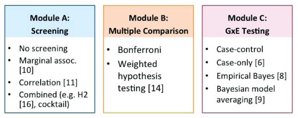
We propose to group the analysis methods into three modules: a “screening” module for prioritizing SNPs; a “multiple comparison” module for addressing the number of tests performed; and a “testing GxE” module for testing GxE. Figure 1 illustrates examples of these modules. In the screening module, one may choose one or both of the marginal and correlation screening to prioritize SNPs or no screening at all. Since many SNPs are tested for GxE, multiple comparison adjustment is essential in declaring the genome-wide significance. Hence, the module-based approach has a multiple comparison module, which includes various methods for multiple comparisons such as the commonly used Bonferroni correction and the weighted hypothesis testing. Finally, in the GxE testing module, one of the case-control test, case-only or EB test may be used to test GxE for SNPs that pass the screening or in the case of no screening, all of the SNPs. We want to note that the methods listed in each module are meant for illustration, and are not intended to be a complete list. It is easy to see that the methods can be mixed and matched both within and across modules for genome-wide GxE. For example, the approach proposed by Murcray et al. [2011] uses both marginal genetic association and correlation for screening, the Bonferroni correction for SNPs that pass the screening, and the case-control test for GxE testing.
Figure 1.
A flow chart of modules including analysis methods for genome-wide Gene × Environment interactions.
There are several distinctive advantages to this modular approach. First, it offers a comprehensive approach to genome-wide searching for GxE. By exploiting various appealing aspects of different methods, such combinations often are substantially more powerful than each individual method on its own under a wide range of scenarios. For example, a two-stage analysis, using the more efficient EB test for GxE, can further gain power compared to the original two-stage analysis that uses the case-control test under most scenarios. Second, because of the modular nature, it also allows investigators to tailor the combination of methods that are specific to their own studies. For example, for GWAS in clinical trials where G and E (say, treatment) are independent due to randomization, the case-only test may be preferred as it can take a full advantage of the independence assumption to gain efficiency. Third, it provides great flexibility to incorporate new methods or extensions of current methods. Finally, the modular approach organizes many existing methods for GxE in a conceptually straightforward fashion. Because it is modular based, little specialized programming is needed beyond that of each individual method.
However, one must be careful with mix-and-matching methods across modules. If GxE test statistics are correlated with screening test statistics, the significance for GxE test statistics may be distorted if the screening is not appropriately adjusted for. Generally it is convenient if the multiple comparison adjustment does not need to consider the screening process besides the number of SNPs that are formally tested for GxE. To do so, it requires that the screening test statistics be independent of GxE test statistics [Dai et al., 2010].
We systematically examine (in)dependence of each of the screening test statistics (marginal association and correlation) in the screening module and each of the GxE test statistics (case-control and case-only) in the GxE testing module. Briefly, we find that the marginal association screening is independent of both the case-control and the case-only tests for GxE, regardless of whether or not confounders are present or the environmental risk factor is continuous. We also find that the correlation screening is independent of the case-control test, but not the case-only test. If one does not want to go through the calculations for deriving proper formulas for the GxE testing accounting for the screening process, these results suggest that we may use any of the case-control, the case-only, or the EB test to test GxE if it is the marginal association screening, but only the case-control test if it is correlation screening. A detailed proof of the (in)dependence between screening and GxE test statistics is provided in the Supplementary Materials.
COCKTAIL METHODS
Following the modular approach, we propose two “cocktail” methods, which use a combined screening approach (marginal association and correlation) to rank the SNPs and test GxE by following the weighted hypothesis testing framework based on the ranking of the SNPs. Both the case-control and EB tests are used for GxE, depending on whether the SNP is chosen based on the correlation screening or marginal association screening. The first cocktail method is aimed to ensure that the screening test is independent of the GxE test, which requires one to pre-specify a threshold to decide which screening method to use. To avoid the potential arbitrariness in choosing the threshold, we propose a second cocktail method. However, in this method, the screening test is not independent of the GxE test. Fortunately, we do not need to be concerned about the non-independence in this case, as we are able to show that the non-independence between the screening and GxE tests in fact makes the GxE test conservative, not anti-conservative. Hence, the power may be reduced but the type I error is well controlled.
Specifically, let and be the p-values for the marginal association and the correlation screening test statistic for the ith SNP, respectively for i = 1,…,m. In the first cocktail method, which is denoted by Cocktail-I, the p value for screening is defined as
where c is a pre-specified threshold, Ind(·) is the indicator function, and the superscript screen(I) refers to the screening p-value for Cocktail-I. The screening p value uses primarily the marginal association p value. However, if the p value for the marginal association is large, say greater than c, the screening p value will then be assigned to the correlation screening p value. This is to cover the situation that SNPs with GxE interaction do not result in marginal genetic association but may still be correlated with E. Clearly, the screening p value can also be modified by using the correlation p value as the primary screening and then supplemented by the marginal association p value. However, in our simulation the power for this combination is often less than where the primary screening is based on marginal association (results not shown).
Although we want to take advantage of the more powerful EB test for GxE interaction, we need to avoid inducing the dependence between the screening and testing statistics. In order to do that, we propose to use the EB test only if , i.e. , and the case-control test otherwise. We use EB rather than the case-only test, because it is robust against possible correlation between SNPs and environmental risk factors in the population. In randomized clinical trials, the case-only estimator can replace EB in the cocktail procedure if E is the randomized factor. Specifically, the p-value for testing GxE is defined as
Here the superscript G × E(I) refers to the p-value for GxE for Cocktail-I. We show that and are independent (see Appendix A). This means that we only need to adjust for the number of SNPs that are formally tested for GxE if the top SNP approach is taken [Dai et al., 2010]. To perform the weighted hypothesis testing, we can rank the SNPs based on the screening p-value pscreen(I) and assign the weight by e.g., using the strategy proposed by Ionita-Laza [2007], see the Results section for more details. The independence between and implies that we do not need to be concerned about the ranking process while testing GxE.
To avoid pre-specifying a potentially arbitrary threshold c in , we propose a second cocktail method, which is denoted by Cocktail-II. For this method, we define the screening p value as following:
Here the superscript screen(II) refers to the screening p-value for Cocktail-II. For Cocktail-II, the screening p-value is the marginal genetic association p-value if it is smaller than the correlation screening p-value, and the correlation-based p-value otherwise. Similar to Cocktail-I, the GxE testing uses EB or case-control tests, depending on whether the SNP is selected based on or . Specifically, the p value for GxE test is defined as
For the Cocktail-II method, screening and testing are not independent. This is because when is used, it is under the condition that and is not independent of . Fortunately, this non-independence does not inflate the type I error of the GxE test. In fact, the GxE test is slightly conservative. This is because the correlation screening test statistic and the case-only GxE test statistic (therefore also the EB test) are positively correlated. When the EB is used for testing GxE when the correlation p-value is greater than or equal to the marginal p-value, the type I error is less than or equal to the expected level, which means that the GxE test based on in Cocktail-II is conservative. The detail of the proof is provided in Appendix B.
Like Cocktail-I, we may use the weighted hypothesis testing by using the screening p-value pscreen(II) to rank the SNPs and assign the weight accordingly. The conservativeness of Cocktail-II may result some power loss. However, from the simulation results presented below, we see that the power loss, if any, is very modest, and in fact, in some cases there is a slight gain in power.
RESULTS
METHODS COMPARISON
We conducted a simulation study to evaluate the performance of our two cocktail methods and other possible combinations according to the proposed modular approach. These methods are listed in Table I. For each screening approach (no screening, correlation, and marginal association abbreviated by No, Corr, and Marg, respectively), the GxE test can be case-control (CC), case-only (CO), or EB. Either the Bonferroni correction for all SNPs (Bonf), top SNPs (Top), or the weighted hypothesis testing (Wt) may be used to adjust for multiple comparisons. Here “top SNPs” refers to using a cut-off value (e.g., a p-value threshold) for screening tests to select top SNPs. For example, a test with name of “Corr-Top-CC” uses correlation for screening and the case-control test for GxE with Bonferroni correction for top SNPs. Three combination approaches, H2, Cocktail-I and Cocktail-II, are also listed in Table I. The H2 approach was recently proposed by Murcray et al. [2011]. It uses both correlation and marginal association for screening, followed by CC test for GxE. Using our naming convention, H2 would be named as Comb-Top-CC, where “Comb” refers to a combined screening approach. Cocktail-I and Cocktail-II would be named as Comb-Wt-CC/EB with different combined screening approaches. Clearly, within each module, other methods could be used. For example, instead of using EB to test GxE, one may also use the Bayesian averaging method [Li and Conti, 2008]. To avoid cluttering, we do not exhaust all possibilities. We note that the choices we made here are fairly representative and expect that the conclusions based on these simulation results generally hold for similar types of combinations.
Table I.
Combinations of methods for genome-wide GxE and the summary of type I error for when there is no correlation (no corr) and modest correlation (modest corr) between SNPs and G, respectively. Inflated type I error rates are bolded
| Name | Screening | GxE Interaction | Multiple Testing | Type I Error |
|
|---|---|---|---|---|---|
| No Corr | Modest Corr | ||||
| No-Bonf-CC | No | Case-Control | Bonferroni correction | 0.040 | 0.043 |
| No-Bonf-CO | Case-Only | for all SNPs | 0.032 | 0.653 | |
| No-Bonf-EB | EB | 0.014 | 0.016 | ||
| Corr-Top-CC | Correlation | Case-Control | Bonferroni correction | 0.048 | 0.045 |
| Corr-Top-CO | Case-Only | for SNPs that pass | 1.000 | 1.000 | |
| Corr-Top-EB | EB | correlation screening | 0.459 | 0.505 | |
| Corr-Wt-CC | Correlation | Case-Control | Weighted testing | 0.048 | 0.048 |
| Corr-Wt-CO | Case-Only | for all SNPs ranked | 0.999 | 1.000 | |
| Corr-Wt-EB | EB | by correlation | 0.384 | 0.315 | |
| Marg-Top-CC | Marg assoc | Case-Control | Bonferroni correction | 0.052 | 0.044 |
| Marg-Top-CO | Case-Only | for SNPs that pass | 0.040 | 0.102 | |
| Marg-Top-EB | EB | marg assoc screening | 0.025 | 0.030 | |
| Marg-Wt-CC | Marg assoc | Case-Control | Weighted testing | 0.038 | 0.046 |
| Marg-Wt-CO | Case-Only | for all SNPs ranked | 0.039 | 0.209 | |
| Marg-Wt-EB | EB | by marg assoc | 0.025 | 0.030 | |
| H2 | Correlation & | Case-Control | Bonferroni for SNPs | 0.047 | 0.043 |
| (Comb-Top-CC) | Marg assoc | that pass both screening | |||
| Cocktail-I | Correlation & | Case-Control & | Weighted test for all SNPs | 0.032 | 0.049 |
| (Comb-Wt-CC/EB) | Marg Assoc | EB | ranked by pscreen(I) | ||
| Cocktail-II | Correlation & | Case-Control & | Weighted test for all SNPs | 0.031 | 0.046 |
| (Comb-Wt-CC/EB) | Marg Assoc | EB | ranked by pscreen(II) | ||
For selecting top SNPs for testing GxE, we set the p-value threshold 10∗3 for the screening test statistics. The same threshold is also used as c in Cocktail-I. For the H2 method, an equal allocation, i.e., 5 × 10⁻⁴, was taken for the two screening approaches. The Bonferroni correction will be adjusted for the top SNPs. For the weighted hypothesis testing, we adopted the strategy proposed by Ionita-Laza et al. [2007] with the initial group size K = 5. According to the strategy, the ranked SNPs are grouped as follows: the first group consists of the first 5 SNPs, the second group consists of the next 10 SNPs, the third group consists of the following 20 SNPs, so on and so forth until all SNPs are assigned. Then the corresponding group-level significance thresholds are α/2, α/4, α/8, …. One can see that this will control the overall type I error since α/2 + α/4 + α/8 + … < α. Within each group, the individual SNP significance threshold is calculated using a Bonferroni correction. For example, for the first group, the threshold for individual SNPs is (α/2)/5 with 5 being the number of SNPs in the first group, and for the second group, the threshold is (α/4)/10 with 10 being the number of SNPs in the second group, and so forth.
Figure 2 shows a schematic plot of the significance thresholds for the Bonferroni correction for all SNPs, the Bonferroni correction for only top SNPs, and the weighted hypothesis testing. In contrast to the constant threshold for the Bonferroni correction either for all or top SNPs, the threshold of the weighted hypothesis testing is monotonically more stringent with the rank of the SNPs.
Figure 2.

A schematic plot of significance levels for three multiple testing methods. Bonferroni correction for all the SNPs assuming a total of 100,000 SNPs are genotyped (Bonferroni, green dot-dash line); Bonferroni correction for the top 100 SNPs (Top SNP, blue dash line); and weighted hypothesis testing using the grouping scheme proposed by Ionita-Laza et al. (2007) with initial group size K=5 (Weighted testing, red solid line). X-axis is the ranking of the SNPs.
SIMULATION SCENARIOS
We generated one dichotomous environmental covariate denoted by E with Pr(E = 1) = 0.5 and odds ratio (OR) = 1.5, representing a moderate environmental effect. We generated a total of 100,000 SNPs. For simplicity, we assumed SNPs were binary variables with frequencies randomly generated from Uniform[0.1,0.4]. Among these SNPs, we randomly selected 10 SNPs having main effects with no GxE effect on disease risk. The ORs of the main effects were generated from Uniform[1.1, 1.8], mimicking the moderate genetic effect of common variants that have been identified in GWAS. We generated a small amount of correlation in the data with each SNP having 0.5% probability to be correlated with E, where the log(OR) of the correlation was generated from a normal distribution with mean 0 and variance {log(1.5)/2}2. Hence, the correlation is very modest: 95% of times when SNPs and E are dependent, the OR for correlated SNPs is from 0.67 to 1.5. We also considered the situation of no correlation at all, that is, all of the SNPs are independent of E. A logistic regression model was used to generate disease status, including the environmental covariate, E, and the 10 associated SNPs. The intercept in the model was set to be −7, to yield about 1 in 1000 disease incidence. Since there is no SNP having interaction effects, this simulation scenario was used to assess the type I error.
To assess power of the methods we used the same set-up, but generated one SNP that had a GxE. We denote this SNP by G to differentiate from SNPs that have no interaction effects. We assumed G was a binary variable with Pr(G = 1) = 0.5. We simulated scenarios where G was and was not correlated with E in the population. For the correlated scenario, we considered both positive (OR = 1.20) and negative (OR = 0.83) correlations. Two types of GxE models were considered:
Synergistic interaction model: The OR of developing a disease in individuals with (G=1, E=1) is much greater than in individuals with (G=0, E=0), (G=1, E=0), or (G=0, E=1). For simplicity, we assumed no main genetic effect and considered a series values for the interaction effect with exp(β) = 1.5, 1.75, 2, 2.25, and 2.5.
Qualitative interaction model: The OR of developing a disease in individuals with G=1 compared to those with G=0 are in opposite direction in the exposed (E=1) and unexposed group (E=0). We considered a series of values for the interaction effect, exp(β) = 1.5, 1.75, 2, 2.25, and 2.5. We let the magnitude of the odds ratio in the exposed increases by the same amount as that decreased in the unexposed group; this can be achieved by setting the main genetic effect to 2/{1 + exp(β)}. Note that this is a rather extreme situation, as it results in no genetic marginal effects at all.
Under each setting, a total of 2000 data sets, each consisting of 1000 cases and 1000 controls, were generated.
TYPE I ERROR
Table 1 shows the type I error of all methods considered at an overall level 0.05 when none of the SNPs is correlated with E (no corr) and when there is a moderate correlation (modest corr) where inflated type I error rates are bolded. It can be seen that the type I error of the correlation-based screening followed by either case-only or EB tests for GxE are greatly inflated, even when none of the SNPs is correlated with E, hence, these combinations cannot be recommended for use. The case-only approach has inflated type I error if there is a correlation between SNPs and E. The EB tests, on the other hand, control the type I error well under all scenarios. All hybrid approaches, H2, Cocktail-I, and Cocktail-II maintain the correct type I error. The type I error of H2, Cocktail-I, and Cocktail-II are 0.047, 0.032, and 0.031 when there is no correlation between SNPs and E, respectively, and 0.043, 0.049, and 0.046, respectively when there is a modest correlation. As expected, Cocktail-II is slightly more conservative than Cocktail-I.
POWER COMPARISON
For the power comparison, we omitted methods that do not maintain the correct type I error, as power for these methods may look artificially greater than other methods due to inflation of the type I error. The omitted methods are all approaches that use case-only tests for GxE, and the correlation-based screening followed by the EB test. We describe the results of power comparison of the following methods: No-Bonf-CC, No-Bonf-EB, Corr-Top-CC, Marg-Top-CC, Marg-Top-EB, Corr-Wt-CC, Marg-Wt-CC, Marg-Wt-EB, H2, Cocktail-I, and Cocktail-II. Supplementary Figure S1, S2 and S3 show the power comparison for these methods, when G and E are independent, positively correlated, and negatively correlated, respectively.
Among the methods being compared, two general patterns are consistently observed. First, the EB test for GxE is considerably more powerful than the CC test when G and E are independent, regardless whether it is synergistic or qualitative model, whether screening is performed or not, or whether it is the Bonferroni correction or the weighted testing. When G and E are positively correlated, a smaller gain is observed for EB; however, when G and E are negatively correlated, the EB estimator loses a small amount of power compared to CC. In this case, the EB estimator behaves more like the CC test, though still having some weight on the case-only test, the latter of which would lose power if G and E were negatively correlated.
Secondly, the weighted hypothesis testing gains power compared with the top SNP approach under both correlation and marginal association screening. One reason for the power gain is that highly ranked SNPs have a lower significance threshold in weighted testing than in the top SNP approach. That said, we want to point out that the power of both approaches depends on the threshold or the group size choices. For the top SNP approach, Murcray et al. Murcray et al. [2011] examined carefully the effect of the threshold on sample size requirement for GxE, and noted that a robust choice can be made across various scenarios. We observed a similar phenomenon in our simulation, for both the top SNP threshold and the threshold c in the Cocktail I method. We set 10−3, which, for a 100,000 marker panel here, brings about 100 SNPs to test for interaction. This number is in line with the threshold used in Murcray et al. [2011], in which the threshold was set to 10−4 for 1,000,000 SNPs, also yielding about 100 SNPs for interaction testing. For weighted testing we tried other choices for the initial group size (K=10 and 20) and found that the power is also relatively invariant.
To further investigate the differences of power between methods, we selected the best performing method from each category under most scenarios: no screening (Bonf-EB), correlation-based two-stage analysis (Corr-Wt-CC), marginal association two-stage analysis (Marg-Wt-EB), and the three hybrid methods (H2, Cocktail-I, and Cocktail-II). The power of these methods is shown in Figure 3, 4 and 5, when G and E are independent, positively correlated, and negatively correlated, respectively.
Figure 3.

Power comparison of the methods when G and E are independent. The X-axis is the odds ratio for the interaction e ect and the Y-axis is the power. The odds ratio for the main e ect of E is 1.5 and for G is 1 under the synergistic model. Under the qualitative model, the odds ratio for the main e ect of G is 1/1+OR(interaction). (a) Synergistic interaction model and no correlation between null markers and E; (b) Qualitative interaction model and no correlation between null markers and E; (c) Synergistic model and modest correlation between null markers and E; (d) Qualitative model and modest correlation between null markers and E. The results are based on a total of 2000 simulated data sets, each consisting of 1000 cases and 1000 controls.
Figure 4.

Power comparison of the methods when G and E are positively correlated with odds ratio 1.2. The X-axis is the odds ratio for the interaction effect and the Y-axis is the power. The odds ratio for the main effect of E is 1.5 and for G is 1 under the synergistic model. Under the qualitative model, the odds ratio for the main effect of G is 1/1+OR(interaction). (a) Synergistic interaction model and no correlation between null markers and E; (b) Qualitative interaction model and no correlation between null markers and E; (c) Synergistic model and modest correlation between null markers and E; (d) Qualitative model and modest correlation between null markers and E. The results are based on a total of 2000 simulated data sets, each consisting of 1000 cases and 1000 controls.
Figure 5.

Power comparison of the methods when G and E are negatively correlated with odds ratio 0.83. The X-axis is the odds ratio for the interaction effect and the Y-axis is the power. The odds ratio for the main effect of E is 1.5 and for G is 1 under the synergistic model. Under the qualitative model, the odds ratio for the main effect of G is 1/1+OR(interaction). (a) Synergistic interaction model and no correlation between null markers and E; (b) Qualitative interaction model and no correlation between null markers and E; (c) Synergistic model and modest correlation between null markers and E; (d) Qualitative model and modest correlation between null markers and E. The results are based on a total of 2000 simulated data sets, each consisting of 1000 cases and 1000 controls.
Under the synergistic interaction model, the two-stage analysis that uses the marginal association as screening (Marg-Wt-EB) has the best power, particularly when a modest correlation is present between null markers and E. No screening (Bonf-EB) has the lowest power. The power of the correlation-based screening falls between that of Marg-Wt-EB and Bonf-EB. In contrast, under the qualitative interaction model, the marginal association screening has the lowest power while the correlation-based screening has the best power with Bonf-EB in between. This is due to the hypothesized qualitative interaction model, which results in no genetic marginal effect. Therefore, the marginal association screening is unable to place G among the top SNPs to be brought to the second stage for interaction testing.
Among the hybrid methods, the power of the proposed Cocktail-I and Cocktail-II methods are consistently very close to the best performing method under all scenarios, whether the interaction effect is synergistic or qualitative, the null markers are or are not correlated with E, or G is or is not correlated with E. The H2 method Murcray et al. [2011] generally has less power than the cocktail methods. For example, under the synergistic model when there is no correlation between the null markers and E and also between G and E, the best power is from Marg-Wt-EB, which is 0.970. In the same scenario, the power for Cocktail-I and II is 0.968 and 0.962, respectively, and the power for H2 is 0.736 (Table II). For another example, under the qualitative interaction model with a modest correlation between the null markers and E, OR(G,E)=1.20, the correlation screening with weighted hypothesis testing, Corr-Wt-CC, gives the best power, 0.890. The Cocktail-I and Cocktail-II methods give power 0.879 and 0.884, respectively, and H2 gives power 0.686 (Table III). The H2 method is closer to the better performing of the methods that uses the top SNP approach, Corr-Top-CC and Marg-Top-CC, see Supplementary Figure 1–3. We also modified the H2 method by using the weighted testing. The power is now similar to the Cocktail methods under the qualitative model, but less under the synergistic model. The reason is that under the synergistic model, the marginal screening is usually more powerful than the correlation screening, and for marginal screening, the cocktail which uses EB to test GxE is more powerful than the H2 which uses the case-control test (results not shown).
Table II.
Power comparison under both synergistic and qualitative interaction models, and when G and E are independent, positively correlated, and negatively correlated, respectively. The odds ratio for the main effect of E is 1.5. For G it is 1 under the synergistic model and 0.62 under the qualitative model. The interaction effect is 2.25. There is no correlation between null markers and E. The results are based on a total of 2000 simulated data sets, each consisting of 1000 cases and 1000 controls.
| Synergistic Interaction |
Qualitative Interaction |
|||||
|---|---|---|---|---|---|---|
| OR(G,E) | OR(G,E) | |||||
| Name | 1.00 | 1.20 | 0.83 | 1.00 | 1.20 | 0.83 |
| Bonf-CC | 0.225 | 0.212 | 0.228 | 0.230 | 0.234 | 0.238 |
| Bonf-EB | 0.544 | 0.476 | 0.149 | 0.555 | 0.478 | 0.156 |
| Corr-Top-CC | 0.754 | 0.790 | 0.299 | 0.606 | 0.784 | 0.074 |
| Corr-Wt-CC | 0.882 | 0.925 | 0.433 | 0.726 | 0.922 | 0.196 |
| Marg-Top-CC | 0.782 | 0.786 | 0.778 | 0.008 | 0.011 | 0.002 |
| Marg-Top-EB | 0.916 | 0.871 | 0.765 | 0.010 | 0.012 | 0.002 |
| Marg-Wt-CC | 0.920 | 0.923 | 0.916 | 0.046 | 0.060 | 0.036 |
| Marg-WT-EB | 0.970 | 0.956 | 0.920 | 0.195 | 0.276 | 0.016 |
| H2 | 0.736 | 0.734 | 0.724 | 0.566 | 0.725 | 0.072 |
| Cocktail-I | 0.968 | 0.956 | 0.916 | 0.676 | 0.914 | 0.178 |
| Cocktail-II | 0.962 | 0.938 | 0.913 | 0.664 | 0.917 | 0.152 |
Table III.
Power comparison under both synergistic and qualitative interaction models, and when G and E are independent, positively correlated, and negatively correlated, respectively. The odds ratio for the main effect of E is 1.5. For G it is 1 under the synergistic model and 0.62 under the qualitative model. The interaction effect is 2.25. About 5% of null markers have a correlation with E. The results are based on a total of 2000 simulated data sets, each consisting of 1000 cases and 1000 controls.
| Synergistic Interaction |
Qualitative Interaction |
|||||
|---|---|---|---|---|---|---|
| OR(G,E) | OR(G,E) | |||||
| Name | 1.00 | 1.20 | 0.83 | 1.00 | 1.20 | 0.83 |
| Bonf-CC | 0.220 | 0.222 | 0.224 | 0.208 | 0.218 | 0.229 |
| Bonf-EB | 0.532 | 0.464 | 0.150 | 0.560 | 0.469 | 0.136 |
| Corr-Top-CC | 0.712 | 0.736 | 0.309 | 0.586 | 0.754 | 0.066 |
| Corr-Wt-CC | 0.786 | 0.907 | 0.382 | 0.632 | 0.890 | 0.164 |
| Marg-Top-CC | 0.78 | 0.777 | 0.798 | 0.006 | 0.017 | 0.002 |
| Marg-Top-EB | 0.908 | 0.862 | 0.776 | 0.007 | 0.019 | 0.002 |
| Marg-Wt-CC | 0.920 | 0.918 | 0.918 | 0.040 | 0.052 | 0.030 |
| Marg-Wt-EB | 0.970 | 0.954 | 0.928 | 0.187 | 0.274 | 0.014 |
| H2 | 0.727 | 0.714 | 0.730 | 0.540 | 0.686 | 0.063 |
| Cocktail-I | 0.956 | 0.938 | 0.874 | 0.606 | 0.879 | 0.154 |
| Cocktail-II | 0.952 | 0.932 | 0.871 | 0.598 | 0.884 | 0.130 |
We also conducted simulations for when Pr(E) = 0.25 and Pr(E) = 0.75, respectively. Under the qualitative interaction model, as expected, the correlation-based screening is more powerful than the marginal association screening. Under the synergistic interaction model, interestingly, the correlation-based screening is more powerful or as powerful as the marginal association screening when Pr(E) = 0.25, but is considerably less powerful when Pr(E) = 0.75. In either case, both cocktail methods, again, track very well with the best performing method and the difference between the two cocktail methods is minimal (results not shown).
DISCUSSION
In this article, we propose a modular approach to integrating various GxE methods, exploiting each method’s most appealing aspects. Three modules are considered: screening, multiple comparison and GxE testing. We combine all three of these modules and develop two novel “cocktail” methods, Cocktail-I and Cocktail-II. We prove that asymptotically Cocktail-I maintains the correct type I error, while Cocktail-II is conservative. Our simulation studies indeed show that Cocktail-II is slightly more conservative. A major advantage of Cocktail-II compared to Cocktail I is that it does not require pre-specifying any threshold for choosing marginal association or correlation as screening. Generally speaking, the power of the two cocktail methods is similar and both perform very well under all parameter settings considered. For GWAS data where the underlying true GxE interaction models are generally unknown, such cocktail methods are particularly useful.
While the simulation in this paper is focused on binary E, the proposed methods are readily applied to continuous E. The (in)dependence of screening and GxE test statistics is the same for when E is continuous as when E is binary (see Supplementary Materials). One caveat with continuous E is that we can not regress E on G for the case-only test using linear or other simple regression models as the regression coefficient does not have the same interpretation as the GxE interaction in the logistic regression model for the case-control analysis. Instead, we recommend regressing G on E using logistic or polytomous model, as G is always a categorical variable, and under suitable modeling the parameters associated E have the same interpretation as the GxE interaction in the logistic regression model for the case-control analysis and they can be combined to form EB estimators.
For quantitative traits, the cocktail methods may also be used, depending on the sampling scheme of the subjects. For example, if the subjects are sampled from the two extreme tails of the distribution and the data are analyzed as if they were case-control data, the proposed cocktail methods can readily apply. However, if the data are analyzed as continuous given the sampling scheme, the screening strategies may still apply; however the case-only and therefore the EB estimators are not defined. Further work is needed in extending the cocktail methods to quantitative traits.
A common practice for accounting for multiple testing in GWAS is to use a Bonferroni correction in which all SNPs are treated equally. Recently methods have been proposed to up-weight and down-weight hypotheses, based on prior likelihood of association with the phenotype Roeder et al. [2007] or results of grouped analysis of the data Roeder and Wasserman [2009]. The two-stage analysis provides a natural choice for determining the weight based on the screening statistics. Here we used the approach proposed by Ionita-Laza et al. to assign the weight. Our results show that it increases power; in some cases this power gain is up to 30% ~ 40%. A fruitful area of research may be to construct optimal weights based on screening in order to further improve power. Biologic information about SNPs can also be brought in to inform the weights.
The statistical interaction depends on the measure used for describing the association. In this paper it is defined as departure from the multiplicative main effects on the odds of developing disease, which, in the rare disease situation, approximates the disease risk. Biological interaction generally refers to two or more causes of disease that together assert their influence on disease risk. Biological interaction may be manifested in statistical interaction, however they are not equivalent. A statistical interaction can be due to model misspecification such as inadequate fit of main effects or misspecified measures of the association (e.g., additive versus multiplicative effects). Additionally, as with all association analyses, association does not imply causation. For further discussion on statistical interaction and biological interaction, see Thomas [2010] and Gerstman [2003].
GWAS data have offered us an unprecedented opportunity to study the genetic etiology of diseases and how genes may interact with environment. In this article, we show how to combine various methods in a principled way to enhance power for detecting gene-environment interaction. Following these principles, we proposed two cocktail methods and show that they are powerful in detecting GxE under a wide range of scenarios and interaction models. Both methods use complementary information from marginal and correlation screens, while exploiting the more powerful EB test when possible. The method also introduce weighted hypothesis testing rather than the top SNP approach that is more common in two-stage screening designs. A practical aspect of our methods is that they build upon common test statistics and hence are easily implemented, allowing for a broad application to genome-wide scan of GxE. The conceptualization of methods as three modules also allows for an easy extension to incorporate new tests within each category as they are developed. Finally, while the proposed methods are targeted for GxE, they are also applicable to studying gene-gene interactions. Our work opens new possibilities for devising powerful methods for detecting gene-environment and gene-gene interaction.
Supplementary Material
Acknowledgments
Contract grant sponsor: National Institute of Health; Contract grant numbers AG14358, CA53996, HG006124, CA90998, CA137088, CA059045, HG005152.
Appendix A.
Proof of independence between screening pscreen(I) and pG×E(I)
Let α1 and α2 be any value between 0 and 1. We show that under the null hypothesis of no
The last step follows the independence between the marginal association screening test statistic and the case-only test (and therefore the EB test) for the first term, and the independence between the case-control test for GxE and both marginal and correlation screening test statistics for the second term. Under the null hypothesis of no G × E, we have Pr(pEB < α2) = α2 and Pr(pCC < α2) = α2. The type I error for pEB may be slightly inflated when G and E are not independent in the population, although the bias is quite minimal (Mukherjee et al. 2008) and therefore we ignore it here. Then
Therefore, Pr(pG×E(I) < α2|pscreen(I) < α1) = α2. This, with the result from Dai et al (2010), implies that the proposed Cocktail-I method maintains the correct type I error without the need to adjust for the screening.
Appendix B.
Proof that the Cocktail method II is conservative
Let α1 and α2 be any value between 0 and 1, we show that under the null hypothesis of no G × E, Pr(pG×E(II) < α2|pscreen(II) = α1) ≤ α2. This implies that for any given screening p-value = α1, if we control pG×E(II) < α2, the actual type I error is less than α2. So the proposed Cocktail-II test statistic is conservative. In what follows, we sketch out the proof. First, we rewrite the joint probability of pscreen(II) and pmarg(II) as
| (1) |
The last equation is a result of the independence of the marginal association estimators from both the case-control and case-only estimators for the interaction, and also from the correlation estimator between G and E in combined cases and controls (see Supplementary Materials for the proofs of these independences). We have also shown that the case-only estimator of interaction and the correlation estimator are asymptotically positively correlated. Since the EB estimator is a weighted sum of case-only and case-control estimators for GxE, the EB estimator is also positively correlated with the correlation estimator asymptotically. Hence, we have
Under the null hypothesis of no G × E, the probability Pr(pEB < α2) = α2 and Pr(pCC < α2) = α2. Plugging them into (1) and with the above inequality, we see that
Therefore, Pr(pG×E(II) < α2|pscreen(II) = α1) ≤ α2. We prove that the type I error for the Cocktail-II method is in fact smaller than the pre-determined value α2. In other words, the Cocktail-II method is conservative.
Footnotes
Additional Supporting Information may be found in the online version of this article.
SUPPLEMENTARY MATERIALS Supplemental materials include proofs of asymptotic correlations between the estimators used in screening test statistics and the estimators used in GxE test statistics. They also include three figures of power comparison of all methods.
References
- Albert PS, Ratnasinghe D, Tangrea J, Wacholder S. Limitations of the case-only design for identifying gene-environment interactions. Am J Epidemiol. 2001;154:687–693. doi: 10.1093/aje/154.8.687. [DOI] [PubMed] [Google Scholar]
- Dai JY, Kooperberg C, LeBlanc M, Prentice RL. On two-stage hypothesis testing procedures via asymptotically independent statistics. University of Washington Biostatistics Working Paper Series; 2010. Paper 367. [Google Scholar]
- Gerstman BB. Epidemiology kept simple: an introduction to traditional and modern epidemiology. Wiley-Liss Inc; New Jersey: 2003. [Google Scholar]
- Ionita-Laza I, McQueen MB, Laird NM, Lange C. Genomewide weighted hypothesis testing in family-based association studies, with an application to a 100K scan. Am J Human Genet. 2007;81:607–614. doi: 10.1086/519748. [DOI] [PMC free article] [PubMed] [Google Scholar]
- Kooperberg C, LeBlanc M. Increasing the power of identifying gene-gene interactions in genome-wide association studies. Genet Epidemiol. 2008;32:255–263. doi: 10.1002/gepi.20300. [DOI] [PMC free article] [PubMed] [Google Scholar]
- Li D, Conti L. Detecting gene-environment interactions using a combined case-only and case-control approach. Am J Epidemiol. 2008;169:497–504. doi: 10.1093/aje/kwn339. [DOI] [PMC free article] [PubMed] [Google Scholar]
- Murcray CE, Lewinger JP, Gauderman WJ. Gene-environment interaction in genome-wide association studies. Am J Epidemiol. 2009;169:219–26. doi: 10.1093/aje/kwn353. [DOI] [PMC free article] [PubMed] [Google Scholar]
- Murcray CE, Lewinger JP, Conti DV, Thomas DC, Gauderman WJ. Sample size requirements to detect gene- environment interactions in genome-wide association studies. Genet Epidemiol. 2011;35:201–210. doi: 10.1002/gepi.20569. [DOI] [PMC free article] [PubMed] [Google Scholar]
- Mukherjee B, Anh J, Gruber SB, Chatterjee N. Testing gene-environment interaction in large scale case-control association studies: Possible choices and comparisons. Am J Epidemiol. 2011 doi: 10.1093/aje/kwr367. in press. [DOI] [PMC free article] [PubMed] [Google Scholar]
- Mukherjee B, Chatterjee N. Exploiting gene-environment independence for analysis of case-control studies: An empirical Bayes-type shrinkage estimator to trade-off between bias and efficiency. Biometrics. 2008;64:685–694. doi: 10.1111/j.1541-0420.2007.00953.x. [DOI] [PubMed] [Google Scholar]
- Piegorsch WW, Weinberg CR, Taylor J. Non hierarchical logistic models and case-only designs for assessing susceptibility in population-based case-control studies. Stat Med. 1994;13:153–162. doi: 10.1002/sim.4780130206. [DOI] [PubMed] [Google Scholar]
- Roeder K, Wasserman L. Genome-wide significance levels and weighted hypothesis testing. Stat Sci. 2009;24:398–413. doi: 10.1214/09-STS289. [DOI] [PMC free article] [PubMed] [Google Scholar]
- Roeder K, Wasserman L, Devlin B. Improving power in genome-wide association studies: Weights tip the scale. Genet Epidemiol. 2007;31:741–747. doi: 10.1002/gepi.20237. [DOI] [PubMed] [Google Scholar]
- Rothman N, Garcia-Closas M, Chatterjee N, Malats N, Wu X, Figueroa JD, Real FX, Van Den Berg D, Matullo G, Baris D, Thun M, Kiemeney LA, Vineis P, De Vivo I, Albanes D, Purdue MP, Rafnar T, Hildebrandt MA, Kiltie AE, Cussenot O, Golka K, Kumar R, Taylor JA, Mayordomo JI, Jacobs KB, Kogevinas M, Hutchinson A, Wang Z, Fu YP, Prokunina-Olsson L, Burdett L, Yeager M, Wheeler W, Tardn A, Serra C, Carrato A, Garc?a-Closas R, Lloreta J, Johnson A, Schwenn M, Karagas MR, Schned A, Andriole G, Jr, Grubb R, 3rd, Black A, Jacobs EJ, Diver WR, Gapstur SM, Weinstein SJ, Virtamo J, Cortessis VK, Gago-Dominguez M, Pike MC, Stern MC, Yuan JM, Hunter DJ, McGrath M, Dinney CP, Czerniak B, Chen M, Yang H, Vermeulen SH, Aben KK, Witjes JA, Makkinje RR, Sulem P, Besenbacher S, Stefansson K, Riboli E, Brennan P, Panico S, Navarro C, Allen NE, Bueno-de-Mesquita HB, Trichopoulos D, Caporaso N, Landi MT, Canzian F, Ljungberg B, Tjonneland A, Clavel-Chapelon F, Bishop DT, Teo MT, Knowles MA, Guarrera S, Polidoro S, Ricceri F, Sacerdote C, Allione A, Cancel-Tassin G, Selinski S, Hengstler JG, Dietrich H, Fletcher T, Rudnai P, Gurzau E, Koppova K, Bolick SC, Godfrey A, Xu Z, Sanz-Velez JI, D Garca-Prats M, Sanchez M, Valdivia G, Porru S, Benhamou S, Hoover RN, Fraumeni JF, Jr, Silverman DT, Chanock SJ. A multi-stage genome-wide association study of bladder cancer identifies multiple susceptibility loci. Nat Genet. 2010;42:978–984. doi: 10.1038/ng.687. [DOI] [PMC free article] [PubMed] [Google Scholar]
- Smith PG, Day NE. The design of case-control studies: the influences of confounding and interaction effects. Int J Epidemiol. 1984;13:356–365. doi: 10.1093/ije/13.3.356. [DOI] [PubMed] [Google Scholar]
- Thomas DC. Gene-environment-wide association studies: emerging approaches. Nat Rev Genet. 2010;11:259–272. doi: 10.1038/nrg2764. [DOI] [PMC free article] [PubMed] [Google Scholar]
- The Wellcome Trust Case Control Consortium Genome-wide association study of 14,000 cases of seven common diseases and 3,000 shared controls. Nature. 2007;447:661–678. doi: 10.1038/nature05911. [DOI] [PMC free article] [PubMed] [Google Scholar]
Associated Data
This section collects any data citations, data availability statements, or supplementary materials included in this article.