

Abstract
Mass spectrometry (MS)-based shotgun proteomics allows protein identifications even in complex biological samples. Protein abundances can then be estimated from the counts of MS/MS spectra attributable to each protein, provided that one corrects for differential MS-detectability of the contributing peptides. We describe the use of a method, APEX, which calculates Absolute Protein EXpression levels based on learned correction factors, MS/MS spectral counts, and each protein's probability of correct identification.
The APEX-based calculations consist of three parts: (1) Using training data, peptide sequences and their sequence properties, a model is built that can be used to estimate MS-detectability (Oi) for any given protein. (2) Absolute abundances of proteins measured in an MS/MS experiment are calculated with information from spectral counts, identification probabilities and the learned Oi -values. (3) Simple statistics allow for significance analysis of differential expression in two distinct biological samples, i.e., measuring relative protein abundances. APEX-based protein abundances span more than four orders of magnitude and are applicable to mixtures of hundreds to thousands of proteins from any type of organism.
Keywords: Quantitative proteomics, Protein expression, Label-free mass spectrometry, Spectral counting
1. Introduction
Mass spectrometry (MS) based shotgun proteomics is a fast and relatively easy method for large-scale protein identification. A typical shotgun proteomics experiment proceeds by tandem MS (MS/MS) analysis of peptides from proteolytically digested proteins, followed by in silico matching of the observed MS/MS spectra against a database of theoretical peptide spectra derived from the expected protein sequences. Typical database search engines include SEQUEST or MASCOT (see also Chapter 28). Proteins are identified through combined evidence for their contributing peptides, resulting in a list in which each protein is associated with a confidence score (or probability) of correct identification, e.g., from ProteinProphet (1). In addition, an MS dataset provides information on the types and number of different peptide spectra associated with each protein, as well as peak heights corresponding to ion intensities.
A number of approaches have been developed to quantify protein observations from peak heights in shotgun proteomics experiments by introducing internal reference standards, often by addition of isotopically labeled peptides (2, 3) (for summary see Chapter 7). These reference standards can be derived from cells grown in labeled medium, as in SILAC (4) (see Chapters 13 and 14), by derivatizing natural samples, as in ICAT (5), or can instead be synthesized and added to samples, as in isotope dilution (e.g., AQUA (6)) (see Chapter 17). The necessity (and expense) of synthesizing thousands of isotopically labeled peptides has prevented easy scaling to full proteomes, even when employing unlabeled peptides (7).
Thus, development of label-free quantitation methods for mass spectrometry has been of high interest. Peak intensities have been used to estimate protein concentrations, e.g., through average the intensities of contributing peptides (8, 9) (see Chapter 16). Other approaches have considered quantitation from the MS/MS sampling statistics in a shotgun proteomics experiment (see Chapter 22). Both the coverage of unique peptides in a protein (i.e., percentage of possible peptides per protein actually observed) and the total number of repeat observations of MS/MS spectra from all peptides in a protein (spectral count) approximate protein abundance (10–17). However, both measures have shortcomings, such as coverage showing saturation (at 100%), spectral counts not accounting for protein size (larger proteins contribute more peptides), both approaches ignoring sampling depth, i.e., the total number of MS/MS experiments that go into the calculation, and neither approach considering the prior odds of observing any particular peptide in the experiment, i.e., the MS-detectability. Peptides vary considerably in their ability to be detected by an MS instrument due to, for example, chemical sequence properties that affect peptide ionization (18). Although such trends can be partly predicted from a peptide's amino acid composition (19–25), many quantitation approaches have not incorporated these predictions to adjust observed spectral counts.
Here, we present protocols for implementing a quantitative method, called APEX (Absolute Protein EXpression index) which addresses each of these limitations using protein identification scores, spectral counts and prior estimates of the number of unique tryptic peptides expected for the protein (Oi value) to calculate absolute protein expression indices (26). We estimate the Oi value employing machine learning techniques accounting for protein size, sequence properties, ionizability and other properties influencing MS detectability. The number of MS/MS spectra observed in the experiment, i.e., repeat peptide observations, is then normalized by the Oi value for each protein, i.e., the number of unique peptides expected, and serves as an estimate of the protein's abundance. In addition, we normalize by the total number of spectra observed in the experiment to enable comparison between experiments with different sampling depths.
APEX is a robust and rapid method to quantify absolute protein abundance. It is appropriate for large-scale protein expression measurements where absolute abundance estimates are desirable and especially where isotope-labeling is impractical. In comparison to intensity-based methods, it is an extremely easy and still reliable method. In contrast to other non-MS-based techniques (27–30), APEX can be used for large-scale datasets and differential protein expression without construction of fusion protein libraries, labeling, or internal standards.
APEX-based protein abundances span over four orders of magnitude and are applicable to mixtures of hundreds to thousands of proteins sampled from any organism of known sequences (26). We developed and tested APEX on two different electrospray ionization MS instruments (ThermoFinnigan Surveyor/DecaXP + iontrap (LCQ), ThermoFinnigan LTQ-Orbitrap); however, the method is equally applicable to other MS instruments. We successfully applied APEX to proteomes of yeast (26), Escherichia coli, Pseudomonas aeruginosa (31), mouse (26), Mycobacterium (32), Arabidopsis (33), rice (31), as well as human (34). Related methods based on spectral counting were used, for example, for the fission yeast (35), worm, and fl y proteome (36).
2. Materials
2.1. Equipment
Mass spectrometry data of peptides. Raw data needs to be postprocessed using MS analysis software of choice (see below). For model training (Subheading 3.2.1), a well-de fined MS dataset is necessary for which several proteins are confidently identified (or known to be present).
Mac, PC, or Linux/Unix workstation.
Amino acid sequences for proteins of interest, e.g., FASTA file.
Information on amino acid properties, e.g., aaindex1 file from ftp://ftp.genome.jp/pub/db/community/aaindex/.
Files/scripts from the APEX Web site, http://www.marcottelab.org/APEX_Protocol/.
2.2. Setup
Software to analyze MS raw data (Sequest, Mascot; PeptideProphet (37) and ProteinProphet (1), see http://tools.proteomecenter.org/TPP.php).
Scripting language for text parsing (e.g., Perl, Python). For a collection of example Perl scripts, see http://www.marcottelab.org/APEX_Protocol/.
WEKA (http://www.cs.waikato.ac.nz/∼ml/weka/) machine learning software.
Alternatively to Setup 2 and 3: the APEX Quantitative Proteomics Tool installed on Windows PC, freely downloadable from http://pfgrc.jcvi.org/index.php/bioinformatics/apex.html (38).
3. Methods
3.1. General Practice
This protocol describes APEX in three sections (Fig. 1). First, using a high-quality MS dataset, vectors of sequence features, and machine learning techniques, we build a computational model that is able to predict peptide MS detectability (see Subheading 3.2.1). The resulting model is organism- and sequence-independent and can be reused for any set of sequences analyzed on the same MS instrument. That means that Subheading 3.2.1 can be omitted in future analyses if a suitable model is available. Then, we predict protein MS detectability (Oi -values) as the sum of the respective peptide MS detectabilities predicted using the model and amino acid sequence features (see Subheading 3.2.2). This section is similar to Subheading 3.2.1 with respect to preparation of the input data files. However, peptide observations are not known but predicted using the model created in Subheading 3.2.1. Again, once Oi -values have been calculated for a particular set of sequences and experimental setup, this step can be omitted in future analyses.
Fig. 1.
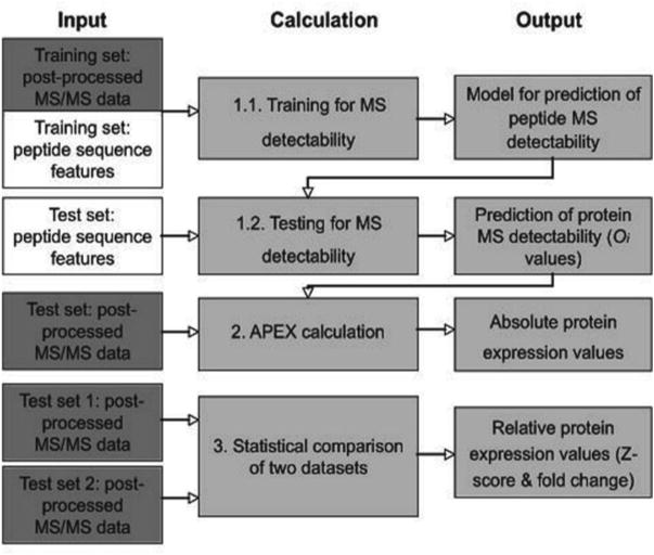
APEX pipeline—overview. The protocol describes three different calculations. (1) Using training MS/MS data, a model is created to describe peptide MS detectability. This model is then used to predict peptide MS detectability for any test data file. (2) Using Oi -values (summed probabilities of peptide MS-detectability) and MS/MS data, we calculate APEX, an estimate of absolute protein expression. (3) Two MS/MS data files can be statistically compared calculating a Z -score. Fold-changes of expression levels are based on APEX estimates described in step 2. Reprinted from ref. 39 with permission from Macmillan Publishers Ltd.
Second, using postprocessed mass spectrometry data, Oi -values for the detected proteins and an estimate of the total number of molecules per cell (C), we calculate indices of absolute protein expression (APEX) for a given protein i (see Subheading 3.3).
Third, for detection of relative protein abundances in two different samples, we present a test for statistically significant differential protein expression (Fig. 1). The statistical test (Z -score) is based only on spectral counts; for an estimate of expression fold change between the two samples, APEX expression values need to be calculated as described in Subheading 3.3.
We describe this protocol with the example of yeast cell lysate analyzed on the LTQ-Orbitrap Classic (Thermo). Additional information may also be obtained from ref. 39. On the APEX Web site (http://www.marcottelab.org/APEX_Protocol/), we provide input and output files created during the process, a suite of corresponding Perl scripts, as well as data for analysis. [Squared brackets] in this text mention Perl scripts corresponding to the described step in the analysis. We also provide example data for training and prediction of MS detectability of E. coli, P. aeruginosa, yeast, rice, mouse, and human proteins both for the LTQ-Orbitrap and/or an LCQ Deca Plus, as well as a Z -score analysis of yeast grown in minimal and rich media. The models trained on these (or other) datasets can analyze data of any origin if the same parameters have been used for data postprocessing.
In our example analysis, we train prediction of peptide MS detectability on a set of 89 yeast proteins which are well-observed in an LTQ-Orbitrap MS/MS experiment, and then estimate Oi values for all proteins in the entire yeast genome. As an example, the TFC3 protein (YAL001C) has ∼500 theoretical peptides from a tryptic digest with ≤ 2 missed cleavages. Only four different pep-tides are observed in the given MS/MS dataset with a total of five spectral counts (Fig. 2). Given the sequence properties of all ∼500 contributing peptides and a trained model, TFC3's Oi value is 60.24, i.e., about 60 peptides are expected for this protein to be observed in an LC-MS/MS analysis on an LTQ-Orbitrap. With an average of 4,000 molecules/protein and a total of 2,033 proteins detected in total, the APEX value for TFC3 is estimated to be ∼110 molecules/cell.
Fig. 2.
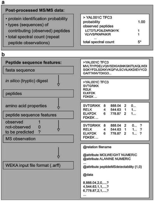
Preparation of input files. We use two basic types of input data. (a) Postprocessed MS/MS-data from which information on the probability of correct protein identification (pi), the types of contributing (observed) peptides and the number of their MS/MS spectral observations is extracted A total of five MS/MS spectra map to the example protein, YAL001C. (b) Sequence feature data calculated for in silico digested protein sequences using known amino acid features. The feature vectors can be extended to any length; the most important features are described in literature (24, 26). The example protein YAL001C is described for a prediction of peptide MS detectability; for its peptides the panels list the length, molecular weight and two arbitrary features. Reprinted from ref. 39 with permission from Macmillan Publishers Ltd. Asterisk—total spectral count per protein
3.2. Training and Testing of a Model for Prediction of Peptide and Protein MS Detectability
3.2.1. Training
If not already done so, postprocess MS/MS raw data with software of choice (e.g., Sequest or Mascot, and PeptideProphet (37)/ProteinProphet (1)) and parse for proteins of confident identification (e.g., false discovery rate <5%). The final output lists should be available in the .xml and –prot.xml file format to be parseable with our Perl scripts [np_parse_ProteinProphet.pl].
From these proteins, select a set of ∼30–150 proteins identified at high confidence (see Note 1). Even for these well-identified proteins, not all theoretically possible peptides will be observed. A comparison of the sequence properties of the observed versus the nonobserved peptides mapping to these proteins is used for training of the computational model (Fig. 2a).
Digest the amino acid sequences for the proteins in silico into (tryptic) peptides, for example using Proteogest (40) at http://www.utoronto.ca/emililab/proteogest.htm . Trypsin cleaves after lysine (K) or arginine (R) unless they are followed by pro-line (P) (Fig. 2b). In silico digestions usually account for 0, 1, or 2 missed cleavages per peptide. Missed cleavages strongly increase the number and types of peptides per protein, i.e., they impact the respective Oi value. In our example, we include up to 2 missed cleavages; however, we observe zero missed cleavages for most peptides, i.e., the tryptic digest appears to be nearly complete. If only one or zero missed cleavages are to be allowed, the model should be rebuilt accordingly. For model building, it is sufficient to digest only the proteins in the training dataset; however, we typically digest the whole proteome and then select the respective training proteins (see APEX Web site for Perl scripts). The choice of the maximum allowed number of missed tryptic cleavages should be the same for training, testing and application of APEX.
Describe sequence features (attributes) for all peptides [np_peptide_properties.pl] (see Note 2). Attributes should include the peptide length (number of amino acids) and the amino acid frequencies (relative and absolute). Attributes can also include the molecular weight, number of unique theoretical peptides, hydrophobicity, solubility, solvent accessibility, etc. or features identified by Mallick et al. (24) to characterize proteotypic peptides. We collected all amino acid features from the AAindex (http://www.genome.jp/aaindex/). Attributes can be numerical, continuous or categorical. Consistent with Mallick et al.'s work, we include both the sum and the average values for any amino acid characteristic as a peptide feature.
For each of the peptides assign “1” if it has been observed in the selected proteomics data (step 2) and, “0” if it has not been observed. When using Peptide- and ProteinProphet output, observation of a peptide is marked as “Contributing_peptide=‘Y’” in the –prot.xml file.
Convert the peptide feature vectors including MS observation (1, 0) into WEKA .arff file format (Fig. 2b) which lists all features (attributes) in the order in which they occur in the feature vector, as well as the feature vectors in form of comma separated values [np_arf_to_arff_TRAINING.pl] (see Note 5). The file format does not contain peptide identifiers; they need to be stored separately. Note that they could be kept in the file, but would have to be unselected in the WEKA explorer prior to training.
Create a model of peptide MS detectability using WEKA (see Notes 4, 6). The process requires a lot of computer memory (depending on the size of the training set), thus we recommend allocating extra memory to WEKA when opening it or using the command line options. Here, we describe the steps to be taken with WEKA Explorer Java user interface. To open WEKA and allocate 500 MB memory, enter “java -Xmx512m -jar < your directory here>/weka.jar.” Computing times quoted here are obtained allocating 1,800 MB of memory to WEKA with no other processes running.
-
In WEKA, load the .arff file in the “Preprocess” tab (Fig. 3a) and then switch to “Classify” (Fig. 3b). Select classifiers in the “Classifier—Choose” option: first select CostSensitive Classifier under “meta” classifiers. Then, select in the popup window bagging under “meta” classifiers. Click on the text bar listing Bagging and select RandomForest under “meta” classifiers. Of course, one can chose not to use Bagging or to use a different classifier. However, in our experience this performs best.
Within the popup window for the CostSensitive Classifier, define a “costMatrix” (see Note 3). Cost-sensitive training is crucial as the training dataset is heavily biased towards one class (e.g., here 91% of nonobserved peptides) and a cost matrix counteracts this bias by weighted use of the training data. Adjust the matrix size to 2. In our example, the cost matrix looks like as follows:
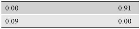
It implies that during learning, the contribution of true-positives, i.e., observed peptides, is weighted as 91% while they represent only 9% of the data. Vice versa, true-negatives, i.e., nonobserved peptides, represent 91% of the data and are down-weighted in their contribution. The cost matrix can also be saved and uploaded in later uses. Specify 10 in the Cross-Validation tab for tenfold cross-validation.
Start calculations by clicking on “Start.” Depending on computer power and dataset size, model building with cross-validation takes several minutes.
-
The output file contains information on the success of the training (Fig. 3c). For example, the F -measure which is the weighted harmonic mean of precision and recall [2 × precision × recall/(precision + recall)] of class prediction. The closer the F -measure is to 1, the larger are the precision and recall and the better is the prediction. In many training sets, most peptides are not observed; prediction of peptide observation is harder than prediction of nonobservation. Therefore, we recommend paying special attention to the F -measure (as well as precision, recall) of observed peptides (class 1); the larger this F -measure, the better is the model. The F -measure should be >0.5.
In the yeast example, observed peptides (class 1) are predicted with an F -measure of 0.61, i.e., with precision and recall of 0.59 and 0.63, respectively. Nonobserved peptides (class 0) are predicted with much higher precision (0.96) and recall (0.96), and the F -measure is 0.96.
-
Once the training is finished and a quality model has been created (see Note 8), save the model as a .model file by right-clicking in the “Results list” section and selecting “Save model.”
Subheading 3.2.1 can be omitted if a model has been built and saved in previous calculations for a particular MS instrument and setup (see Notes 7, 9, and 10). We found that models are similar between MS instruments using the same ionization method and mass range, and the resulting Oi values correlate strongly. However, since, for example, an LCQ is less sensitive than an LTQ-Orbitrap, Oi values are generally smaller on the former instrument than on the latter.
Fig. 3.
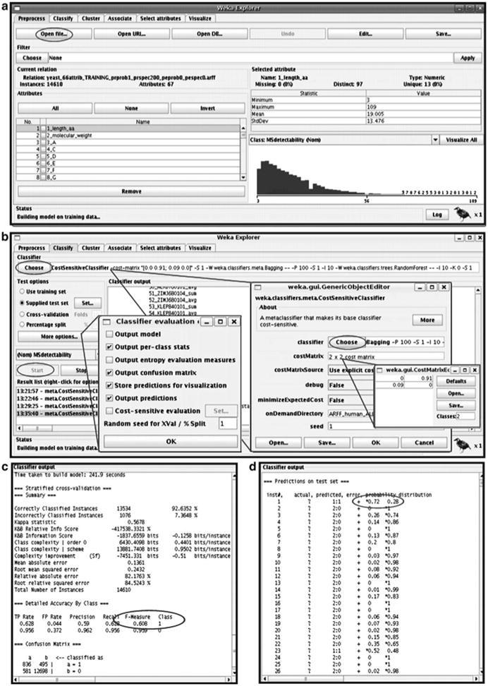
Use of WEKA. The screenshots illustrate how use of the WEKA Explorer can look like. Ovals mark steps described in this protocol. (a) Uploading the .arff file. (b) Choosing the classifier and defining cost matrix and other parameters. (c) Training output. (d) Prediction output. Reprinted from ref. 39 with permission from Macmillan Publishers Ltd.
3.2.2. Testing (Predictions)
Postprocess MS/MS raw data as in Subheading 2.1, item 1 (Fig. 2a) to obtain –prot.xml files. This time include all proteins of interest, e.g., with <5% false discovery rate. Parse the file to obtain a tab-delimited text file [np_parse_ProteinProphet.pl].
Digest the amino acid sequences for all proteins of interest (above) in silico into (tryptic) peptides, using the same parameters as in Subheading 3.2.1, step 3, i.e., allow for the same number of missed cleavages. Beware that this file easily becomes large; a yeast genome with ∼6,000 genes in silico digests into ∼921,000 peptides (≤2 missed cleavages).
Analyze all peptides for their sequence features using the same attributes as in Subheading 3.2.1, step 4 [np_peptide_properties.pl].
Convert peptide feature vectors into WEKA .arff file format similar to Subheading 3.2.1, step 6 [np_arf_to_arff_TEST.pl]. At the end of each feature vector, place a question mark “?” instead of the “1” or “0” describing peptide observation (Fig. 2b).
Predict probability of observation (peptide MS detectability) using WEKA. In the “Preprocess” tab, load the .arff file created in step 4. In the “Classify” tab, load the model created in Subheading 3.2.1 by right-clicking within the “Result list” section and choosing “Load model.” If you do not yet have a model available, create it according to Subheading 3.2.1 Select CostSensitive Classifier, Bagging, and Random Forests as classifiers and de fine a cost matrix as described in Subheading 3.2.1, step 8. Do not select Cross-Validation. Select the “Supplied test set” option and upload the test .arff file, i.e., the file for which you like to obtain predictions. Under “More Options,” unselect to output the model and select to display the output predictions. After loading the existing model, right-click within the “Result list” section and select “Re-evaluate existing model with current dataset.”
Start calculations by clicking on Start. Depending on computer power and dataset size the calculations can take several minutes.
Cut and paste the output file into a text file or save it by right-clicking in the “Result list” section and selecting “Save result buffer.” The second but last column of the output file provides the probability of peptide observation (Fig. 3d), i.e., the class 1 probability, and this value is used for further calculations. Note that while peptide MS detectability is binary during training (observed/nonobserved), it is continuous when calculating Oi (class 1 probability: value between 0 and 1).
-
Match the peptide identities to probabilities of peptide observation of the WEKA output file [np_PeptidePredictions_to_ProteinOi.pl]. Sum over the probabilities for all peptides mapping to a protein; this sum is the Oi value of the protein, i.e., the expected number of observed peptides. Store these Oi values in a data file.
Once calculated for an organism for a particular experimental setup, the Oi values can be reused for any number of MS/MS analyses of the same proteins. The APEX Web site provides Oi values for the entire proteomes of E. coli, yeast and human for analysis on an LCQ and an LTQ-Orbitrap using a given protocol, mass range, etc. (provided on the APEX Web site).
3.3. Estimation of Absolute Protein Expression Levels
Postprocess MS/MS raw data as described in Subheading 3.2.1, step 1. For each protein identified in the MS/MS experiment, we need the probability of correct identification pi and the total number of observed MS/MS spectra ni. Parse the –prot.xml file to obtain a tab-delimited text file [np_parse_ProteinProphet.pl].
Calculate Oi values for each protein as described in Subheading 3.2.2, i.e., the expected number of unique peptides per protein corrected by the differential peptide MS detectability.
Estimate the total number of protein molecules per cell C . A total of 5 × 10⁷ molecules/cell for yeast (29) and 2−3 × 10⁶ molecules/cell for E. coli (41, 42) have been suggested. This total number of molecules will be split amongst the proteins identified in the MS experiment. Since the number of proteins identified can vary between different experiments, an alternative way to estimate C is to multiply the number of proteins identified by an estimate of the average number of molecules per protein. For yeast, an average of ∼2,000–10,000 molecules per protein is expected (26, 27, 29), for E. coli < 1,000 (26, 41, 42). In our example experiment, 2,033 proteins were identified with <5% false discovery rate on the LTQ-Orbitrap; thus, we estimate C = 2,033 proteins × 4,000 molecules/protein ≈ 8.1 × 10⁶ molecules. Third, if not cellular lysates but a synthetic protein mixture is used, C can be estimated using the total concentration of proteins in the sample (if known). Fourth, C can also be set to a constant (e.g., 1 or 100) which results in APEX values of proteins relative to each other in the sample. Note that this use of the term relative differs from that in Subheading 3.4 which considers a protein's abundance in two different samples.
-
Calculate APEX protein absolute protein expression values using Eq. 1 [np_APEX_from_Oi_and_protlist.pl].
1 In Eq. 1, ni is the total spectral count for protein i (total number of MS/MS spectra attributable to protein i), Oi is the expected unique peptide count for protein i (sum of peptide MS detectabilities for a given protein), and pi is the protein identification probability. Values for ni and pi are extracted from postprocessed MS/MS data; Oi is computed as described above.
As a control for correct APEX calculations, we that recommend the user conducts a spike-in experiment as described in the original publication (26). In such an experiment, a mixture of proteins of known abundances is spiked into cellular lysate and APEX is used to estimate protein concentrations in the mixture. This control experiment may be conducted once in the lab to assure that the setup produces reliable estimates of protein concentrations. It does not have to be repeated frequently.
3.4. Estimation of Relative Protein Expression (Comparison of Two Samples)
Postprocess MS/MS raw data of both samples as described in Subheading 3.2.1, step 1, including parsing of the –prot.xml files [np_parse_ProteinProphet.pl]. For each protein identified in the MS/MS experiment, we need the probability of correct identification pi and the total number of observed MS/MS spectra ni.
Calculate APEX-based protein abundance estimates as described in Subheading 3.3 [np_APEX_from_Oi_and_protlist.pl]. The expression fold change between the two samples 1 and 2 can then be expressed as the ratio APEXi,1/APEXi, 2. If a protein is absent in one sample, its spectral count is ni = 0 and an APEX-based fold-change cannot be calculated. However, a Z -score describing the significance of the expression change can always be calculated.
Calculate the total number of observed MS/MS spectra (total spectral counts) N for each sample. This sum includes only peptides of confident identification (above threshold). Convert the spectral counts ni into fractions fi = ni/N.
Calculate for each protein the overall proportion fi,0 = (ni,1 + ni,2)/(N1 + N2). The proportion fi,0 is the null expectation in the event that protein i is present at the same level in both samples. The calculation can be done for proteins which are confidently identified in both samples, and for proteins which are only identified in one sample but assumed to be absent in the other sample.
-
Calculate for each protein a Z -score of differential expression according to
2 where N1 and N2 are the total spectral counts in samples 1 and 2, fi,0 is the overall proportion of a protein's spectral counts, and fi,1 and fi,2 are the proportions of a protein's spectral counts in sample 1 and 2, respectively. Note that script [np_two_ files_ Zscore.pl] performs steps 3–5 and provides Z -scores as the output of a comparison of two .apex files.
Two-sided P -values require |Z| > 1.96 for P -value < 0.05; |Z| > 2.58 for P -value < 0.01. Proteins of high abundance in both samples can be significantly differentially expressed even if the actual expression fold-change is small. Thus, we recommend examining both Z -scores and expression fold-changes for each protein. The APEX Web site contains an example of differential protein expression analysis (yeast grown in minimal versus rich medium).
Table 1.
Features used for training. The number and types of peptide sequence attributes is important for performance of the training/testing of peptide MS detectability. Except for length, all amino acid attributes and their descriptions originate from AAindex (http://www.genome.jp/aaindex/). For all attributes except for length and amino acid composition, both total (sum) and average values along sequence are included in the description of peptide properties (.arf and .arff files)
| Attribute type | Source (reference number in AAindex) | Comment |
|---|---|---|
| Length | ||
| Molecular weight Fasman (43) | FASG760101 | Strongly correlated with Length (can be left out to reduce redundancy) |
| Relative amino acid frequencies | Instances of type of amino acid in sequence divided by length | |
| Absolute amino acid frequencies | Instances of type of amino acid in sequence | Correlated with Length |
| Normalized frequency of alpha-helix Chou Fasman (44) | CHOP780201 | Secondary structure |
| Normalized frequency of beta-sheet Chou Fasman (44) | CHOP780202 | Secondary structure |
| Normalized frequency of beta-turn Chou Fasman (44) | CHOP780203 | Secondary structure |
| Propensity to be buried inside Wertz Scheraga (45) | WERD780101 | Main attribute for MUDPIT-ESI identified by Mallick et al. (24) |
| Isoelectric point Zimmerman et al. (46) | ZIMJ680104 | Main attribute for MUDPIT-ESI identified by Mallick et al. (24) |
| Net charge Klein et al. (47) | KLEP840101 | Main attribute for MUDPIT-ESI identified by Mallick et al. (24) |
| Atom-based hydrophobic moment Eisenberg McLachlan (48) | EISD860102 | Main attribute for MUDPIT-ESI identified by Mallick et al. (24) |
| Positive chargeFauchere et al. (49) | FAUJ880111 | Main attribute for MUDPIT-ESI identified by Mallick et al. (24) |
| Normalized flexibility parameters (B -values), average Vihinen et al. (50) | VINM940101 | Additional attribute |
| Normalized van der Waals volume Fauchere et al. (49) | FAUJ880103 | Additional attribute |
| Apparent partition energies calculated from Chothia index Guy (51); Amino acid side-chain partition energies and distribution of residues in soluble proteins | GUYH850105 | Additional attribute |
| Transfer energy, organic solvent/water Nozaki Tanford (52) | NOZY710101 | Additional attribute |
Acknowledgments
C.V. acknowledges support by the International Human Frontier Science Program. We thank John Braisted and Srilatha Kuntumalla from JCVI for many useful discussions regarding the APEX calculations. This work was supported by grants from the Welch (F-1515) and Packard Foundations, the National Science Foundation, and National Institutes of Health (to E.M.M.).
Abbreviations
- APEX
Absolute Protein EXpression
- MS
Mass spectrometry
- MS/MS
Tandem mass spectrometry
Footnotes
Selection of high-quality training data.
High-quality training data is crucial for successful model building and model performance. The training set of proteins (and its size) should be chosen so that (1) recall and precision (F -measure) in cross-validation are maximized (see Subheading 3.2, step 10); and (2) time for model calculation is within desired time frame. In general, the larger the fraction of observed versus nonobserved peptides in the data (i.e., the larger the number of true-positives compared to true-negatives), the better is the model performance. This fraction seems more important than the actual number of proteins (or peptides) selected to be in the training dataset (∼30–150). However, the larger the training dataset, the more time is required to build a model.
We usually select a training dataset based on high protein identification probabilities as well as high spectral counts per protein from a trusted dataset. The protein identification probabilities are an output from the ProteinProphet (1) software. If the user decides not to use Peptide- and ProteinProphet, training proteins could be selected based on high scores obtained in the primary database search (with SEQUEST, MASCOT, or similar) (see Chapter 28). Alternatively, training proteins could be chosen based on knowledge of their presence in other data (e.g., from Western blot experiments or if using a synthetic mixture). In other words, as long as the user is confident that a certain set of proteins is present in the sample, he or she can compare their observed peptides to their nonobserved peptides and learn MS-detectability from these. For our setup, we found that ion suppression does not seem to play a big role, as the complexity of the mixture (i.e., how many proteins are contained in it) only marginally affects the Oi values.
Usually, we obtained the best model when selecting proteins based on high protein identification probability (e.g., 1.00) and high spectral counts per protein (e.g., >200)—rather than when selecting for high probabilities/spectral counts per peptide. However, note that these cutoffs are MS/MS dataset- and machine-dependent and should be reevaluated for different experimental setups. Our cutoffs provide a guideline for experimentation.
For example, when creating a training file for model for data collected on a Thermo LTQ-Orbitrap, we analyzed yeast cellular lysate identifying 89 proteins of high protein identification probability (pi = 1.00) and with least 200 total spectral counts per protein. For these proteins, 9% (1,331) of the peptides were observed in the MS/MS experiment; 91% (13,279) of peptides were not observed.
The number and types of attributes included is important for model performance.
We observed the best model performance when including a total of 66 attributes (Table 1). These length, molecular weight, relative and absolute amino acid frequencies, secondary structure, five attributes identified by Mallick et al. (24) and four additional attributes. As described by Mallick et al. (24), different instruments, in particular different ionization techniques, require selection of different sequence attributes that influence MS detectability. Assuming that most users may operate a MudPIT ESI type instrument, we focus here on the calculations of Oi values for these.
Training with a cost matrix.
If no cost matrix is specified, model performance is very poor, in particular if there is a strong class bias in training data. The reason lies in the overabundance of true-negatives, i.e., nonobserved peptides. In fact, we recommend reversing or leaving out the cost matrix as a control experiment: decreasing model performance (F -measure) compared to correct use of a cost matrix verifies setup of the calculations. Classifiers other than Bagging and RandomForests may also perform well, as discussed in the original APEX publication (26).
WEKA crashes during training or testing.
The Java-based WEKA explorer uses a lot of memory, especially when handling large files. If WEKA crashes during model building (training), consider allocating more memory or reducing dataset size by filtering the training data more stringently (see Subheading 3.2.1, step 2). Alternatively, use the command-line to set up WEKA runs, avoiding the memory-consuming Java-based interface.
When applying the model to predict peptide MS detect-ability, we found that for a test file with 100,000 lines, at least 1,500 MB memory is required (see Subheading 3.2.1, step 7). If the test file contains more than 100,000 lines, we recommend splitting the file into smaller .arff files, assigning more memory when starting WEKA (see Subheading 3.2.1, step 7) and/or using the WEKA command line interface. For example, the peptide file for the whole yeast genome needs to be split into approximately ten separate .arff files with each 100,000 lines or fewer. Unselect “Output model” under “More options” to save the memory required to output the model.
An error message appears when uploading the .arff training or testing file.
Thoroughly check the .arff file format. Check that the number of attributes listed in the header is the same as the number of attributes (features) in the data rows. Ensure that all rows with data entries have the same number of attributes listed. Check for correct description of attribute types, e.g., as string, numeric or class . Very that rows lack peptide names or other identifiers. If nothing helps, try uploading our example .arff files and work from there.
Training results in a poor model, e.g., the F -measure for observed peptides is <0.5.
Check that the correct cost matrix is used, as described in Subheading 3.2.1, step 8. Check quality of the training data (see Note 1). Consider reducing your training set to fewer proteins, possibly hand-select them for their quality of peptide identification. Check that peptides classified as observed have high peptide identification scores (or probabilities). Check that proteins in the training set are not degenerate, i.e., that several proteins of different names do not map to the same group of peptides. Check that peptides in the training set are not degenerate, i.e., that their observation is not mapped to several proteins of different names. (When selecting our training data, we exclude all degenerate proteins and peptides.) Ensure you use WEKA correctly by training on one of the files provided on the APEX Web site and comparing your training outputs with our result files.
Check types of peptide attributes (see Note 2). Modify the kinds and number of attributes used to describe peptide sequences. Not all 66 attributes used in our example set are equally important for training. Performing different tests in the “Attribute selection” section in WEKA (Ranker-PrincipalComponents, Ranker-InfoGain, and BestFirst-CfsSubset), we identified attributes describing peptide length, the isoelectric point, hydrophobicity, solvent access, solubility, volume, secondary structure as most important, while among amino acid frequencies the number of C, R, and K were top-ranked (see APEX Web site). Consider adding attributes listed by Mallick et al. (24) as important for your experimental setup (if not yet included).
You are unable to use saved/previous WEKA models. Newer WEKA versions are often incompatible with older versions’ models. Thus, one has to retrain the model for the new version of WEKA. Input files are provided on the APEX Web site.
Quality control.
When establishing the APEX protocol, we encourage the reader to use the Perl scripts and sample data files provided on our Web site as a control for correct setup. Probabilities of peptide MS detectability may also be compared to predictions by Mallick et al. (24) and by the Peptide Detectability Predictor at http://darwin.informatics.indiana.edu/applications/PeptideDetectabilityPredictor/. Other tests of the quality of APEX estimates are described in the original publication (26).
When to retrain the model.
A number of additional options are worth keeping in mind. Some users may prefer to retrain the Oi -values for each organism they use, assuming that organism-specific properties (e.g., amino acid composition, the extent of posttranslational modifications) may influence the overall MS-detectability of the peptides. Other users even consider retraining for every experiment. In principle, the Oi -values are robust when similar experimental conditions apply. While a model built on one organism's data might be usable to predict MS-detectability for another other organism, mammalian proteins may, for example, be more heavily phosphorylated than bacterial proteins, and phosphorylation impacts MS-detectability of peptides containing serine, threonine, or tyrosine. In this case, retraining with a mammalian dataset to be used to predict mammalian APEX values is reasonable.
The user should, however, retrain the Oi-values if the mass spectrometry equipment or protocols change. For example, different MS instruments, and in particular different ionization techniques strongly influence MS detectability. Experimental conditions such as oxidization of cysteine residues using iodoacetamide also influence MS detectability of cysteine containing peptides.
Future possible refinements.
We provide this protocol not only for easy calculation of absolute and relative protein expression values but also encourage the reader to experiment and optimize the method to suit his or her needs. Several refinements are possible. For example, when training for peptide MS detectability, actual peptide identification probabilities could be taken into account: instead of using a binary classification (observed, nonobserved) one would use a continuous value. Peptide charge states and prior modifications (e.g., on Cysteine residues) may also be considered. Further, the user may try and estimate how the number of missed cleavages may affect the total number of peptides observed, and incorporate that into the calculation. In addition to charge state, more complex features such as bi-amino acid frequencies may be included in the training process; however, the user should be careful to avoid over fitting, i.e., to have disproportionally many features compared to the size of the dataset.
When including more features, the user should keep two aspects in mind. First, ideally the feature values show a mound-shaped frequency distribution which is easy to check in WEKA. If the distribution is far from Gaussian, one should consider (log) transforming the values to achieve a better distribution. Many learning algorithms require normally distributed feature values. Second, if two features are highly intercorrelated (e.g., Spearman's R > 0.9), for example sequence length and molecular weight, one of the features should be left out to reduce redundancy.
Further information and tools.
For APEX calculations, the primary publication (26) and the APEX protocol (39) provide further help. APEX is also implemented in a free software tool developed by John Braisted and colleagues at the J. Craig Venter Institute, Rockville, MD (38). The software, called the APEX Quantitative Proteomics Tool, is freely available from http://pfgrc.jcvi.org/index.php/bioinformatics/apex.html . We recommend the user to try this Java-based tool. It essentially involves the same steps as described here, but does not require the use of Perl scripts. Using the Perl scripts (and modifying these) allows the user to include further developments such as those described in Note 10.
References
- 1.Nesvizhskii AI, Keller A, Kolker E, Aebersold R. A statistical model for identifying proteins by tandem mass spectrometry. Anal Chem. 2003;75:4646–4658. doi: 10.1021/ac0341261. [DOI] [PubMed] [Google Scholar]
- 2.Oda Y, Huang K, Cross FR, et al. Accurate quantitation of protein expression and site-specific phosphorylation. Proc Natl Acad Sci USA. 1999;96:6591–6596. doi: 10.1073/pnas.96.12.6591. [DOI] [PMC free article] [PubMed] [Google Scholar]
- 3.Ong SE, Mann M. Mass spectrometry-based proteomics turns quantitative. Nat Chem Biol. 2005;1:252–262. doi: 10.1038/nchembio736. [DOI] [PubMed] [Google Scholar]
- 4.Ong SE, Blagoev B, Kratchmarova I, et al. Stable isotope labeling by amino acids in cell culture, SILAC, as a simple and accurate approach to expression proteomics. Mol Cell Proteomics. 2002;1:376–386. doi: 10.1074/mcp.m200025-mcp200. [DOI] [PubMed] [Google Scholar]
- 5.Gygi SP, Rochon Y, Franza BR, Aebersold R. Correlation between protein and mRNA abundance in yeast. Mol Cell Biol. 1999;19:1720–1730. doi: 10.1128/mcb.19.3.1720. [DOI] [PMC free article] [PubMed] [Google Scholar]
- 6.Gerber SA, Rush J, Stemman O, et al. Absolute quantification of proteins and phos-phoproteins from cell lysates by tandem MS. Proc Natl Acad Sci USA. 2003;100:6940–6945. doi: 10.1073/pnas.0832254100. [DOI] [PMC free article] [PubMed] [Google Scholar]
- 7.Ishihama Y, Oda Y, Tabata T, et al. Exponentially modified protein abundance index (emPAI) for estimation of absolute protein amount in proteomics by the number of sequenced peptides per protein. Mol Cell Proteomics. 2005;4:1265–1272. doi: 10.1074/mcp.M500061-MCP200. [DOI] [PubMed] [Google Scholar]
- 8.Silva JC, Gorenstein MV, Li GZ, et al. Absolute quantification of proteins by LCMSE: a virtue of parallel MS acquisition. Mol Cell Proteomics. 2006;5:144–156. doi: 10.1074/mcp.M500230-MCP200. [DOI] [PubMed] [Google Scholar]
- 9.Malmstrom J, Beck M, Schmidt A, et al. Proteome-wide cellular protein concentrations of the human pathogen Leptospira interrogans. Nature. 2009;460:762–765. doi: 10.1038/nature08184. [DOI] [PMC free article] [PubMed] [Google Scholar]
- 10.Kislinger T, Gramolini AO, Pan Y, et al. Proteome dynamics during C2C12 myoblast differentiation. Mol Cell Proteomics. 2005;4:887–901. doi: 10.1074/mcp.M400182-MCP200. [DOI] [PubMed] [Google Scholar]
- 11.Kislinger T, Cox B, Kannan A, et al. Global survey of organ and organelle protein expression in mouse: combined proteomic and transcriptomic profiling. Cell. 2006;125:173–186. doi: 10.1016/j.cell.2006.01.044. [DOI] [PubMed] [Google Scholar]
- 12.Blondeau F, Ritter B, Allaire PD, et al. Tandem MS analysis of brain clathrin-coated vesicles reveals their critical involvement in synaptic vesicle recycling. Proc Natl Acad Sci USA. 2004;101:3833–3838. doi: 10.1073/pnas.0308186101. [DOI] [PMC free article] [PubMed] [Google Scholar]
- 13.States DJ, Omenn GS, Blackwell TW, et al. Challenges in deriving high-confidence protein identifications from data gathered by a HUPO plasma proteome collaborative study. Nat Biotechnol. 2006;24:333–338. doi: 10.1038/nbt1183. [DOI] [PubMed] [Google Scholar]
- 14.Florens L, Washburn MP, Raine JD, et al. A proteomic view of the Plasmodium falciparum life cycle. Nature. 2002;419:520–526. doi: 10.1038/nature01107. [DOI] [PubMed] [Google Scholar]
- 15.Gao J, Friedrichs MS, Dongre AR, Opiteck GJ. Guidelines for the routine application of the peptide hits technique. J Am Soc Mass Spectrom. 2005;16:1231–1238. doi: 10.1016/j.jasms.2004.12.002. [DOI] [PubMed] [Google Scholar]
- 16.Gao J, Opiteck GJ, Friedrichs MS, et al. Guidelines for the routine application of the peptide hits technique. J Proteome Res. 2003;2:643–649. doi: 10.1016/j.jasms.2004.12.002. [DOI] [PubMed] [Google Scholar]
- 17.Liu H, Sadygov RG, Yates JR., 3rd A model for random sampling and estimation of relative protein abundance in shotgun proteomics. Anal Chem. 2004;76:4193–4201. doi: 10.1021/ac0498563. [DOI] [PubMed] [Google Scholar]
- 18.Steen H, Pandey A. Proteomics goes quantitative: measuring protein abundance. Trends Biotechnol. 2002;20:361–364. doi: 10.1016/s0167-7799(02)02009-7. [DOI] [PubMed] [Google Scholar]
- 19.Elias JE, Gibbons FD, King OD, et al. Intensity-based protein identification by machine learning from a library of tandem mass spectra. Nat Biotechnol. 2004;22:214–219. doi: 10.1038/nbt930. [DOI] [PubMed] [Google Scholar]
- 20.Gay S, Binz PA, Hochstrasser DF, Appel RD. Peptide mass fingerprinting peak intensity prediction: extracting knowledge from spectra. Proteomics. 2002;2:1374–1391. doi: 10.1002/1615-9861(200210)2:10<1374::AID-PROT1374>3.0.CO;2-D. [DOI] [PubMed] [Google Scholar]
- 21.Craig R, Cortens JP, Beavis RC. The use of proteotypic peptide libraries for protein identification. Rapid Commun Mass Spectrom. 2005;19:1844–1850. doi: 10.1002/rcm.1992. [DOI] [PubMed] [Google Scholar]
- 22.Kuster B, Schirle M, Mallick P, Aebersold R. Scoring proteomes with proteotypic peptide probes. Nat Rev Mol Cell Biol. 2005;6:577–583. doi: 10.1038/nrm1683. [DOI] [PubMed] [Google Scholar]
- 23.Le Bihan T, Robinson MD, Stewart II, Figeys D. Definition and characterization of a “trypsinosome” from specific peptide characteristics by nano-HPLC-MS/MS and in silico analysis of complex protein mixtures. J Proteome Res. 2004;3:1138–1148. doi: 10.1021/pr049909x. [DOI] [PubMed] [Google Scholar]
- 24.Mallick P, Schirle M, Chen SS, et al. Computational prediction of proteotypic peptides for quantitative proteomics. Nat Biotechnol. 2007;25:125–131. doi: 10.1038/nbt1275. [DOI] [PubMed] [Google Scholar]
- 25.Tang H, Arnold RJ, Alves P, et al. A computational approach toward label-free protein quantification using predicted peptide detectability. Bioinformatics. 2006;22:e481–e488. doi: 10.1093/bioinformatics/btl237. [DOI] [PubMed] [Google Scholar]
- 26.Lu P, Vogel C, Wang R, Yao, et al. Absolute protein expression profiling estimates the relative contributions of transcriptional and translational regulation. Nat Biotechnol. 2007;25:117–124. doi: 10.1038/nbt1270. [DOI] [PubMed] [Google Scholar]
- 27.Ghaemmaghami S, Huh WK, Bower K, et al. Global analysis of protein expression in yeast. Nature. 2003;425:737–741. doi: 10.1038/nature02046. [DOI] [PubMed] [Google Scholar]
- 28.Newman JR, Ghaemmaghami S, Ihmels J, et al. Single-cell proteomic analysis of S. cerevisiae reveals the architecture of biological noise. Nature. 2006;441:840–846. doi: 10.1038/nature04785. [DOI] [PubMed] [Google Scholar]
- 29.Futcher B, Latter GI, Monardo P, et al. A sampling of the yeast proteome. Mol Cell Biol. 1999;19:7357–7368. doi: 10.1128/mcb.19.11.7357. [DOI] [PMC free article] [PubMed] [Google Scholar]
- 30.Lopez-Campistrous A, Semchuk P, Burke L, et al. Localization, annotation, and comparison of the Escherichia coli K-12 proteome under two states of growth. Mol Cell Proteomics. 2005;4:1205–1209. doi: 10.1074/mcp.D500006-MCP200. [DOI] [PubMed] [Google Scholar]
- 31.Laurent J, Vogel C, Kwon T, et al. Protein abundances are more conserved than mRNA abundances across diverse taxa. Proteomics. 2010;23(10):4209–4212. doi: 10.1002/pmic.201000327. [DOI] [PMC free article] [PubMed] [Google Scholar]
- 32.Wang R, Marcotte EM. The proteomic response of Mycobacterium smegmatis to anti-tuberculosis drugs suggests targeted pathways. J Proteome Res. 2008;7:855–865. doi: 10.1021/pr0703066. [DOI] [PubMed] [Google Scholar]
- 33.Baerenfaller K, Grossmann J, Grobei MA, et al. Genome-scale proteomics reveals Arabidopsis thaliana gene models and proteome dynamics. Science. 2008;320:938–941. doi: 10.1126/science.1157956. [DOI] [PubMed] [Google Scholar]
- 34.Vogel C, de Sousa AR, Ko D, et al. Sequence signatures and mRNA concentration can explain two-thirds of protein abundance variation in a human cell line. Mol Syst Biol. 2010;6:400. doi: 10.1038/msb.2010.59. [DOI] [PMC free article] [PubMed] [Google Scholar]
- 35.Schmidt MW, Houseman A, Ivanov AR, Wolf DA. Comparative proteomic and transcriptomic pro filing of the fission yeast Schizosaccharomyces pombe. Mol Syst Biol. 2007;3:79. doi: 10.1038/msb4100117. [DOI] [PMC free article] [PubMed] [Google Scholar]
- 36.Schrimpf SP, Weiss M, Reiter L, et al. Comparative functional analysis of the Caenorhabditis elegans and Drosophila melanogaster proteomes. PLoS Biol. 2009;7:e48. doi: 10.1371/journal.pbio.1000048. [DOI] [PMC free article] [PubMed] [Google Scholar]
- 37.Keller A, Nesvizhskii AI, Kolker E, Aebersold R. Empirical statistical model to estimate the accuracy of peptide identifications made by MS/MS and database search. Anal Chem. 2002;74:5383–5392. doi: 10.1021/ac025747h. [DOI] [PubMed] [Google Scholar]
- 38.Braisted JC, Kuntumalla S, Vogel C, et al. Quantitative proteomics tool: generating protein quantitation estimates from LC-MS/MS proteomics results. BMC Bioinformatics. 2008;9:529. doi: 10.1186/1471-2105-9-529. [DOI] [PMC free article] [PubMed] [Google Scholar]
- 39.Vogel C, Marcotte EM. Calculating absolute and relative protein abundance from mass spectrometry-based protein expression data. Nat Protoc. 2008;3:1444–1451. doi: 10.1038/nport.2008.132. [DOI] [PubMed] [Google Scholar]
- 40.Cagney G, Amiri S, Premawaradena T, et al. In silico proteome analysis to facilitate proteomics experiments using mass spectrometry. Proteome Sci. 2003;1:5. doi: 10.1186/1477-5956-1-5. [DOI] [PMC free article] [PubMed] [Google Scholar]
- 41.Neidhardt FC, Umbarger HE, editors. Escherichia coli and Salmonella typhimurium: cellular and molecular biology. part 4. ASM Press; Washington, DC: 1996. [Google Scholar]
- 42.Sundararaj S, Guo A, Habibi-Nazhad B, et al. The CyberCell Database (CCDB): a comprehensive, self-updating, relational database to coordinate and facilitate in silico modeling of Escherichia coli. Nucleic Acids Res. 2004;32:D293–D295. doi: 10.1093/nar/gkh108. [DOI] [PMC free article] [PubMed] [Google Scholar]
- 43.Fasman GD, editor. Proteins. 3rd. Vol. 1. CRC Press; Cleveland: 1976. Handbook of Biochemistry and Molecular Biology. [Google Scholar]
- 44.Chou PY, Fasman GD. Prediction of the secondary structure of proteins from their amino acid sequence. Adv Enzymol. 1978;47:45–148. doi: 10.1002/9780470122921.ch2. [DOI] [PubMed] [Google Scholar]
- 45.Wertz DH, Scheraga HA. Influence of water on protein structure. An analysis of the preferences of amino acid residues for the inside or outside and for specific conformations in a protein molecule. Macro molecules. 1978;11:9–15. doi: 10.1021/ma60061a002. [DOI] [PubMed] [Google Scholar]
- 46.Zimmerman JM, Eliezer N, Simha R. The characterization of amino acid sequences in proteins by statistical methods. J Theor Biol. 1968;21:170–201. doi: 10.1016/0022-5193(68)90069-6. [DOI] [PubMed] [Google Scholar]
- 47.Klein P, Kanehisa M, DeLisi C. Prediction of protein function from sequence properties: Discriminant analysis of a data base. Biochim Biophys Acta. 1984;787:221–226. doi: 10.1016/0167-4838(84)90312-1. [DOI] [PubMed] [Google Scholar]
- 48.Eisenberg D, McLachlan AD. Solvation energy in protein folding and binding. Nature. 1986;319:199–203. doi: 10.1038/319199a0. [DOI] [PubMed] [Google Scholar]
- 49.Fauchere JL, Charton M, Kier LB, Verloop A, Pliska V. Amino acid side chain parameters for correlation studies in biology and pharmacology. Int J Peptide Protein Res. 1988;32:269–278. doi: 10.1111/j.1399-3011.1988.tb01261.x. [DOI] [PubMed] [Google Scholar]
- 50.Vihinen M, Torkkila E, Riikonen P. Accuracy of protein flexibility predictions. Proteins. 1994;19:141–149. doi: 10.1002/prot.340190207. [DOI] [PubMed] [Google Scholar]
- 51.Guy HR. Amino acid side-chain partition energies and distribution of residues in soluble proteins. Biophys J. 1985;47:61–70. doi: 10.1016/S0006-3495(85)83877-7. [DOI] [PMC free article] [PubMed] [Google Scholar]
- 52.Nozaki Y, Tanford C. The solubility of amino acids and two glycine peptides in aqueous ethanol and dioxane solutions. J Biol Chem. 1971;246:2211–2217. [PubMed] [Google Scholar]